Experiments and simulations of a gravitational granular flow instability

HAL Id: hal-01909770

https://hal.archives-ouvertes.fr/hal-01909770

Submitted on 31 Oct 2018

HAL is a multi-disciplinary open access

archive for the deposit and dissemination of

sci-entific research documents, whether they are

pub-lished or not. The documents may come from

teaching and research institutions in France or

abroad, or from public or private research centers.

L’archive ouverte pluridisciplinaire HAL, est

destinée au dépôt et à la diffusion de documents

scientifiques de niveau recherche, publiés ou non,

émanant des établissements d’enseignement et de

recherche français ou étrangers, des laboratoires

publics ou privés.

flow instability

Jan Vinningland, Øistein Johnsen, Eirik Flekkøy, Renaud Toussaint, Knut

Måløy

To cite this version:

Jan Vinningland, Øistein Johnsen, Eirik Flekkøy, Renaud Toussaint, Knut Måløy. Experiments and

simulations of a gravitational granular flow instability. Physical Review E : Statistical, Nonlinear,

and Soft Matter Physics, American Physical Society, 2007, 76 (5), �10.1103/PhysRevE.76.051306�.

�hal-01909770�

Jan Ludvig Vinningland,1,

*

1_{Department of Physics, University of Oslo, P.0. Box 1048, 0316 Oslo, Norway}

2

Institut de Physique du Globe de Strasbourg, CNRS, Université Louis Pasteur, 5 rue Descartes, 67084 Strasbourg Cedex, France

共Received 1 November 2006; revised manuscript received 28 September 2007; published 27 November 2007兲

An instability is observed as a layer of dense granular material positioned above a layer of air falls in a

gravitational field关Phys. Rev. Lett. 99, 048001 共2007兲兴. A characteristic pattern of fingers emerges along the

interface defined by the grains, and a transient coarsening of the structure is caused by a coalescence of neighboring fingers. The coarsening is limited by the production of new fingers as the separation of the existing fingers reaches a certain distance. The experiments and simulations presented are shown to be comparable both qualitatively and quantitatively. The characteristic inverse length scale of the structures, obtained as the mean of the solid fraction power spectrum, relaxes toward a stable value shared by the numerical and experimental data. Further, the response of the numerical model to changes in various model parameters is investigated. These parameters include the density of the grains, the shape of the initial air-grain interface, and the dissipa-tion of the granular phase. Also, the growth rates of the bulk solid fracdissipa-tion and the air-grain interface are obtained from Fourier power spectra of the numerical data. This analysis reveals that the instability is never in a linear regime, not even initially.

DOI:10.1103/PhysRevE.76.051306 PACS number共s兲: 81.05.Rm, 47.20.Ma, 47.11.⫺j, 45.70.Qj I. INTRODUCTION

Sands and powders are indispensable materials in our modern society. Nevertheless, a complete theoretical descrip-tion of granular materials and their dynamical properties are still not available, despite their widespread use. An improved understanding of granular flows would provide valuable con-tributions to many industrial applications such as pneumatic transport, fluidized beds, and catalytic cracking 关1–3兴.

Granular materials are also involved in a host of natural and geological phenomena, most of which are still in need of a proper understanding. Such phenomena include sedimenta-tion 关4,5兴, erosion and river evolution 关6兴, underwater

ava-lanches and turbidities关7兴, and soil fluidization during

earth-quakes关8兴.

The relatively complete description of classical fluid dy-namics is also useful in the interpretation of granular flows. Instability is a central problem in fluid dynamics关9,10兴, and

over the past few years some classical hydrodynamic insta-bilities have also been reported in granular systems. Ex-amples of such are the Saffman-Taylor instability关11兴 in a

granular suspension关12兴 or in gas-grain mixtures 关13兴, the

Kelvin-Helmholtz instability关14兴 in a vibrated granular

mix-ture 关15兴, the Richtmyer-Meshkov instability in a shock

propagating at the interface between two types of grains关16兴,

as well as some novel instabilities in submarine avalanches 关17兴 and in a tube of sand 关18,19兴. The granular

Rayleigh-Taylor instability discussed here was first reported by the same authors in Ref.关20兴. The present paper provides a more

elaborate and complete discussion of the instability in addi-tion to further results and analyses.

While we study a gas-grain system, the liquid-grain inter-face in a Hele-Shaw cell was investigated experimentally and theoretically by Völtz et al. 关21兴. Sieved glass beads of

80␮m in diameter was used in their experiments, and a

be-havior very similar to the classical Rayleigh-Taylor instabil-ity 关10,22兴 was observed. In contrast, the instability

dis-cussed in this paper arises in a liquid-free granular material and displays processes of tip splitting and finger renucle-ation. Our experimental and numerical data compare favor-ably both qualitatively and quantitatively, despite the two-dimensionality of the model and the neglect of interparticle friction and gas inertia. Linear stability analysis is not ad-equate to predict the final dominating wavelength because nonlinear effects govern the selection of the final wave-length. This is demonstrated explicitly in the numerical data as the growth rates of the solid fraction wave numbers are shown not to follow an exponential growth of any significant duration. The parameter space of the model is explored by changing the density of the grains, the shape of the initial granular interface, and the granular dissipation.

The motivation for the simulations and experiments pre-sented in this paper is to study a granular version of the Rayleigh-Taylor instability关22兴 known from hydrodynamics,

where a dense Newtonian liquid is positioned on top of a less dense liquid in a gravitational field. In our case the dense fluid is replaced by a granular material which, in contrast to the liquid, is not subject to surface tension.

The simulation of two-phase flow is particularly interest-ing for many engineerinterest-ing purposes, and historically most simulations of two-phase flows have treated the solid phase as a continuum, which allowed numerical techniques known from fluid dynamics to be applied. A continuum approach to granular media 共see, e.g., Ref. 关23兴兲 is, however, only

ap-proximate, and will in cases of discontinuous density varia-tions break down completely. Moreover, many interesting phenomena in granular media are closely related to its par-ticularity. A complete description of the interactions between a continuum fluid phase and a discrete solid phase would require the full Navier-Stokes equation for the fluid, coupled with moving boundary conditions given by the surfaces of the grains and the geometry of the container, together with differential equations for the grains. Such a detailed scheme would consume prohibitive computational resources, and a

number of techniques 共see Ref. 关24兴 for a brief summary兲

have been developed in order to reduce the computational efforts while preserving the physics. In contrast, we use a hybrid technique that affords a continuum description of the gas phase and a particulate description of the granular phase. Our model neglects friction, the spatial direction normal to the cell, and the inertia of the air. Yet, this computationally agile model yields results in good agreement with experi-mental observations.

The paper is organized as follows. Section II presents the setup and execution of the experiment, followed by an out-line of the numerical model and its implementation in Sec. III. The numerical and experimental results are presented and analyzed in Sec. IV, which is split into four subsections de-voted to qualitative descriptions of the instability 共Sec. IV A兲, numerical solid fraction and pressure profiles 共Sec. IV B兲, Fourier power spectra and growth rate analysis 共Sec. IV C兲, and the variation of the model parameters 共Sec. IV D兲. The paper is completed with a short conclusion in Sec. V.

II. EXPERIMENT

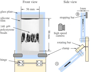
The experimental setup, illustrated in Fig.1, consists of a closed Hele-Shaw cell mounted on a hinged bar which en-ables the cell to rotate 130° from a lower to an upper vertical position共from A to B in Fig.1兲. The Hele-Shaw cell is made

of two 8-mm-thick glass plates clamped onto a 1-mm-thick silicone frame. The internal dimensions of the cell are 56 ⫻86⫻1 mm3_{, and it is filled with polystyrene beads and air} at atmospheric pressure. The cell is rotated manually and it takes about 0.2 s to bring the cell to an upright, vertical position. The off-center pivot of the cell cause the rotation to slow down the falling motion of the grains due to centrifugal forces. A bar is mounted at position B in order to control the final vertical position of the cell. However, this bar has some undesirable side effects, causing nonpersistent perturbations of the initial stages of the instability共see Sec. IV A兲. The full

development of the instability is recorded by a high-speed digital camera共Photron Fastcam-APX 120K兲 taking images with a resolution of 512⫻512 pixels at a rate of 500 frames per second.

Monodisperse polystyrene beads of 140␮m in diameter from Microbeads®共Dynoseeds TS 140-51兲 are used in the experiments. The filling of the cell is performed with one glass plate lying down horizontally and the silicone frame adhered on top. Small portions of beads are carefully depos-ited on the plate and leveled with the silicone frame before the upper plate is attached and fastened with clamps. The cell is flipped a few times after closure to allow the grains to form a random loose-packed configuration.

The humidity in the laboratory is important in order to keep the electrostatic and cohesive properties of the grains at a suitable level to prevent the grains from clustering or stick-ing to the glass plates. Durstick-ing the fillstick-ing of the cell and the execution of the experiment the humidity was kept constant at about 30%.

The experimental results are presented and discussed to-gether with the numerical results in Sec. IV.

III. SIMULATION A. Model

The numerical model is a hybrid model that combines a discrete description of the grains with a continuum descrip-tion of the gas. The foundadescrip-tion and derivadescrip-tion of the model are presented in detail in Refs.关25,26兴; only an outline of the

model is given here.

The granular phase is considered as an agglomeration of spheres that makes up a deformable porous medium which in our model is described by coarse-grained solid fraction

␳共x,y兲 and velocity fields u共x,y兲, where 共x,y兲 are the two-dimensional space coordinates. The continuum gas phase is solely described by its pressure field P共x,y兲; hence the iner-tia and velocity field of the gas are not considered in this model. The focus of the model is to describe the granular flow on a scale of a few grain diameters, not the fluid flow field on a subgranular level. It is justified to neglect the in-ertia of the fluid as long as the Reynolds number is small, which is the case for particles on a micrometer scale sedi-menting in air.

The pressure is governed by the equation关25,26兴

␾

冉

⳵t + u ·⵱P

冊

冉

␬

␮⵱ P

冊

where␾= 1 −␳is the porosity,␳is the solid fraction,␬is the permeability, and u is the velocity field of the granular phase.

P is the gas pressure, and␮ is the gas viscosity. This equa-tion is derived from the conservaequa-tion of air and grain mass, using Darcy’s law 关27兴 to obtain the pressure drop over a

given volume described by a permeability␬. The Carman-Kozeny relation关28兴 is assumed for the permeability, and the

isothermal ideal gas law is assumed for the compressible gas. The empirical Carman-Kozeny relation is given as

high speed camera A B m µ Side view 56 mm hinge glass plate silicone 1mm rotating bar stopping bar 86 mm 140 polystyrene beads Front view clamp film

FIG. 1. 共Color online兲 Illustration of the experimental setup

viewed from the front and the side. Two cell positions are superim-posed in the side view to demonstrate the manual rotation from position A to B.

␬共␳,d兲 = d2 180

共1 −␳兲3

␳2 , 共2兲

where␳ is the local solid fraction, d is the diameter of the grains, and 1/180 is an empirical constant valid for a pack-ing of beads.

The dynamics of the grains are governed by Newton’s second law mdv dt = mg + FI− ⵱P ␳n , 共3兲

where m is the grain mass, v is the grain velocity, FI is the interparticle force which keeps the grains from overlapping,

␳n=␳␳g/m is the number density, and␳gis the mass density of the material the grains are made of. Contact dynamics关29兴

is used to calculate the interparticle force FI but molecular dynamics techniques关30,31兴 could have been used instead.

Contact dynamics is an iterative scheme that calculates the interparticle distribution of normal forces consistent with the kinematic constraints imposed by the impenetrable beads. The solution yields a force network that satisfy volume ex-clusion at every contact. The relative force change from one iterative step to the next is used as a convergence criterion: If the change at every contact is less than a given threshold the solution has converged. The resulting force network shows how the weight of the grains, and possible external forces such as the gas pressure, are transmitted and carried by the grains and the container. More detailed descriptions of con-tact dynamics are found in Refs.关32–34兴. Figure2gives an example a force network obtained in a frictionless packing of 1200 grains relaxed under gravity. The direction and magni-tude of the forces are respectively given by the direction and the thickness of the lines. Typical features of a force network are the heterogeneous distribution of forces and the existence of force chains that transmit a major fraction of the load.

The interparticle and wall-particle friction are not taken into account in this model. The dissipation of the granular phase is controlled by a coefficient of normal restitution,␧,

that determines the loss of kinetic energy associated with each collision.

B. Implementation

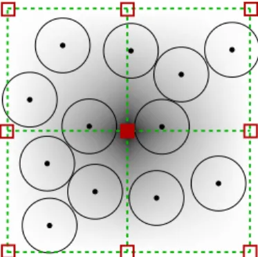
A smoothing function is necessary to translate the mass mi and velocity vi of the individual grains 共indexed by i兲 into continuous solid fraction␳共x,y兲 and velocity fields u共x,y兲 on the grid. A fractional value of mior viis assigned to each of the four neighboring grid nodes and the value is determined by the positional weight of the grain through a linear smoothing function s共r−r0兲 expressed mathematically as 关25兴 s共r − r0兲 =

冦

冉

冊冉

冊

冧

where r共x,y兲 is the position of the grain, r₀共x₀, y₀兲 is the position of the grid node,⌬x=兩x−x₀兩 and ⌬y=兩y−y₀兩 are the relative distances, l is the lattice constant, and 兺ks共r−rk兲 = 1 with k indexing the four sites. The smoothing of the grains is illustrated in Fig.3 where nine grid nodes are de-picted as red squares on a gradient background. This back-ground is the positional weight map of the central node which is shown as a solid square. From this illustration we observe that all the grains in Fig.3make contributions to the field values of the central node: A grain positioned at the central node is assigned a weight of 1共black background兲, while a grain positioned along the dotted outline in Fig.3is assigned a weight of zero 共white background兲. The weight map, or smoothing function, may also be considered as a collection of equidistant tent functions, distributed over the area in Fig.3, with maxima rising linearly from zero to 1 and then back to zero. More explicitly, the number density␳nand average velocity u associated with a node at position r0are, respectively, ␳n共r0兲=兺is共ri− r0兲, and u共r0兲=兺ivis共ri− r0兲, where i runs over the number of particles关25兴.

The positional weight used to obtain the continuous fields is also used to obtain the pressure forces, FP= −⵱P/␳n,

FIG. 2.共Color online兲 Network of interparticle forces FI

calcu-lated by contact dynamics. This image shows the lower right corner of a frictionless packing of 1200 grains relaxed under gravity.

FIG. 3. 共Color online兲 Illustration of the linear smoothing

func-tion used to calculate the continuous fields from the discrete posi-tions and velocities of the grains. The red squares are nodes on the grid, and the gray-level background illustrates the weight map of the central node; black is 1, white is zero.

acting on the grains. Explicitly for a grain at ri, FP= −兺k共⵱P/␳n兲ks共ri− rk兲 with a k index running over the four nodes. In other words, the share of FP assigned to the grain from the node is equal to the share of mior viassigned to the node from the grain.

A few approximations are made in the implementation of the model. The two-dimensional共2D兲 solid fraction of disks is translated into a 3D solid fraction of spheres by multiply-ing the 2D solid fraction with 2/3, which is the ratio of the 3D to the 2D random-close-packed solid fractions. Further, the Carman-Kozeny relation is not valid as the solid fraction approaches zero, and a lower cutoff on the 2D solid fraction,

␳min= 0.25, is introduced. These matters are elaborated in Sec. II C of Ref.关25兴.

The packing of grains used in the simulations is made of 160 000 grains with a mean diameter of 140␮m. This high number of grains is selected to allow a match with the spatial dimensions of the experimental cell. The simulation shown in Fig.4took roughly 12 days to complete on a standard PC. Note, however, that the instability emerges as well in simu-lations with a much more reduced number of grains共e.g., a few thousand兲. The size distribution adopted for the granular packing is flat and has a ±10% variation in the diameter. This minor polydispersity is necessary to avoid a hexagonal stack-ing of the grains.

The granular packing is generated by raining grains from a given height, with random horizontal positions, in a cell without air. After all the grains have settled the packing is allowed to further compactify and relax before the air is in-troduced. This is to prevent the source term of Eq. 共1兲,

−P⵱ ·u, to introduce local pockets of overpressure, due to moving grains, that otherwise could perturb the numerical results.

IV. RESULTS

The rich behavior of the instability provides a number of interesting results which is presented as follows. A

qualita-tive discussion and comparison of the experimental and nu-merical images are given first, followed by solid fraction and pressure profiles from the numerical data in Sec. IV B. A series of investigations, spawned by the Fourier power spec-trum of the solid fraction, is presented in Sec. IV C. These results include a quantitative comparison of the experimental and numerical data, in addition to the temporal evolution of the wave numbers obtained from the solid fraction power spectra. Section IV D investigates the response of the insta-bility to changes in the granular dissipation, the initial air-grain interface, and the air-grain density.

A. Experimental and numerical images

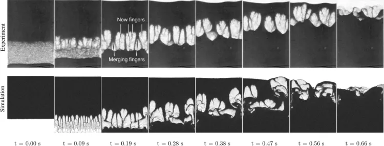
Figure4shows experimental and numerical images of the granular Rayleigh-Taylor instability: A layer of grains dis-placing a layer of air in a gravitational field. The width of both the experimental and numerical system is 56 mm, while the height of the experimental cell is 86 mm, and the height of the numerical cell is 68 mm. The experimental images are color-inverted and contrast-enhanced versions of the original images; the grains are black and the air is white. The time is set to zero when the cell reaches the vertical position. In the experiment some grains start to fall during the rotation of the cell and a small pile of grains has already formed at the bottom of the first frame.

An air-grain interface, initially flat in the simulation but slightly perturbed in the experiment, is defined by the falling grains. When the cell is flipped a pattern of fine fingers emerges along the interface共see Fig.5兲 which subsequently

develop into coarser bubble-finger structures that propagate through the packing. A more detailed analysis of the evolu-tion introduces three stages of development: The first stage is the nucleation stage characterized by a transition from a ho-mogeneous decompaction to the appearance of the first fin-ger seeds. This stage is only observed in the numerical snap-shots because of the reduced initial resolution of the experimental setup: Transient perturbations disturb the initial

Merging fingers New fingers

t = 0.00 s t = 0.09 s t = 0.19 s t = 0.28 s t = 0.38 s t = 0.47 s t = 0.56 s t = 0.66 s

Experiment

Simulation

FIG. 4. Images from the experiment共top row兲 and simulation 共bottom row兲 with polystyrene beads of 140␮m in diameter in a closed

Hele-Shaw cell that is 56 mm wide. The experimental cell is 86 mm high and 1 mm thick, while the numerical cell is 68 mm high. The time of the snapshots is the time evolved since the cell reached the upright position. A restitution coefficient of 0.5 is used in the simulations.

air-grain interface as the rotating cell suddenly stops. The second stage is the growing stage where the nucleated fingers grow in size and start to coalesce with their neighboring fingers. The third and final stage is the propagation stage, which is recognized by the aggregation of grains at the bot-tom of the cell and the formation of bubbles that propagate through the packing. Two competing mechanisms are at play here, one producing finer structures, the other producing coarser structures. The coarsening mechanism causes fingers to merge as two fingers form an inverted Y共see the experi-mental image at t⫽0.19 in Fig. 4兲. The smaller bubble

trapped beneath the wedge of the inverted Y continuously lags behind the bigger bubbles until the small bubble disap-pears. Thus, two fingers have been reduced to one. The other mechanism, giving rise to finer structures, is manifested as thin filaments forming inside the rising bubbles. These new fingers split the bubbles and prevent them from growing in-definitely.

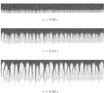
Figure5 shows a more detailed series of numerical snap-shots of the early evolution of the instability: In the top frame the initial homogeneous decompaction of the air-grain interface is visible. By close comparison of the frames it is possible to discern tiny finger seeds in the top frame that has developed into well-defined fingers in the second and third frames. From the second to the third frame the fingers mainly grow in size and only a few new fingers are nucleated. The first and second frame belongs to the nucleation stage, while the third frame is taken from the growing stage.

Figure6shows a snapshot from a simulation where glass beads of 210␮m are used. The beads are colored in bands in their initial configuration to illustrate the dynamics of the mixing and the patterns created by the propagating bubbles. The pattern that emerges is reminiscent of geological pat-terns observed when, e.g., water is forced through sediments of sand关35兴.

A qualitative comparison of the image series in Fig. 4

renders the simulation and experiment consistent in many

respects. The sizes of the bubbles and the fingers are compa-rable, and the dynamical processes of finger merging and finger nucleation are observed in both cases. Nevertheless, some discrepancies are observed, particularly at the start and towards the end of the instability: The initial decompaction, followed by the emergence of the first fine fingers, is only observed numerically. Towards the end of the process a hori-zontal destabilization of the air-grain interface is visible, i.e., some bubbles reach the surface before others.

The initial discrepancies can to a large extent be explained by three experimental features: The increased thickness of the cell allowing up to seven layers of grains between the plates, the rotation of the cell, and the abrupt stop of the cell as it reaches the vertical. Ideally the rotation would be so fast that the grains did not move at all during the rotation. In the experiment this is, however, not the case and the grains will slide and roll down the inclined plate during the rotation while the air passes in a channel above the grains共known as the granular Boycott effect关19兴兲. Only when the cell is

al-most vertical is the sliding layer of grains able to form an interface that fills the whole cross section of the cell so that fingers may start to form. However, a mechanical shock is created in the cell as it hits the bar. The effect is a transverse oscillation that causes the grains to be tossed back and forth between the plates. Any fingers formed prior to the shock will be strongly perturbed and even erased. The result is visible in the first experimental image of Fig. 4 where the falling grains form an almost homogeneous sheet of grains rather than well-defined fingers.

Some differences are also found in the shape of the fin-gers: In the numerical images the fingers appear somewhat buckled and bended compared to the experimental fingers. We believe this is an artifact caused by the cutoff imposed on the solid fraction. Since the solid fraction is not allowed to be less than 0.25, the empty space porosity, i.e., the porosity in a region with no or very few grains, will be different from 1. This again leads to overestimated pressure gradients in the t = 0.02 s

t = 0.04 s

t = 0.06 s

FIG. 5. A closer look at the initial formation of fingers in the simulation. Before the fingers appear there is a transient phase of homogeneous decompaction. Notice the cusp-shaped geometry of the air-grain interface.

FIG. 6.共Color online兲 A snapshot from a simulation using glass

beads of 210␮m in diameter where the initial configuration is

col-ored in horizontal bands to bring out the dynamics of the structures as the instability evolves.

most dilute regions of the system, and forces are exerted on the fingers traversing the gap of air. Nevertheless, the shape of the interface is very well reproduced by the simulations despite the buckling of the fingers.

The experimental instability seems to be more stabilized horizontally than the numerical instability. By comparing im-ages in Fig.4for t⬎0.4 s it is evident that on a detailed level the numerical images are quite different from the corre-sponding experimental images. It seems that the most ad-vanced bubble in the numerical images departs from the other bubbles at an increasing rate, causing a horizontal de-stabilization of the interface. We believe that the reason for this is found in the zero particle-particle friction and, more importantly, the zero particle-wall friction of the numerical model. The friction between the glass plates and the grains in the experiment is probably important in the dense part of the packing, due to the Janssen effect关36兴. This has most likely

a stabilizing effect on the propagation of the interface. How-ever, apart from this small difference in the propagation of the bubbles, the other quantitative features of the instability are well reproduced by our friction-free simulations. Thus, for the sake of simplicity, we have chosen to discard friction in the model. Indeed, taking friction into account would im-ply important numerical costs: The addition of two degrees of freedom to account for the rotation of the grains, and a new fitting parameter for the friction coefficient.

Another effect of zero friction in the simulations is ob-served as the rightmost bubble in the latter numerical images of Fig. 4 reaches the upper surface at about t = 0.45 s and leaves behind an open air-filled void. As grains rush in to fill this void convection rolls are set up that will distort and perturb the present fingers. Such convection rolls would to a large extent be dissipated away if interparticle friction were present in the simulations.

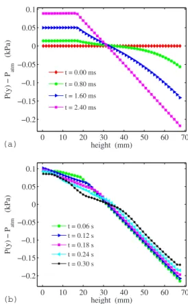
B. Pressure and solid fraction in the simulation The temporal evolution of the pressure P and the solid fraction␳in the simulation are respectively shown in Figs.7

and8. The vertical profiles P共y兲 and␳共y兲 shown for different times are calculated by averaging P共x,y兲 and␳共x,y兲 over the horizontal component x. Figure7共a兲provides a detailed tem-poral description of P共y兲 immediately after the rotation of the cell: The initially flat profile is, within a few millisec-onds, transformed into a linearly decreasing function while an overpressure builds up at the bottom of the cell. This corresponds to a fast diffusion of the pressure field关cf. Eq. 共1兲兴, and shows the transient curvature of the pressure profile

relaxing towards a linear function. This happens at a time scaleᐉ2_{/共Pᐉ␬/␮兲⯝0.1 ms, smaller than the time scale} as-sociated with grain motion due to gravity,

冑

whereᐉ is the system size, and d the grain diameter. Figure

7共b兲shows P共y兲 for later times, and the linearity of the pres-sure in the upper part of the packing, above the air-grain interface, is almost unchanged. Figure8 shows ␳共y兲 for the same times as in Fig.7共b兲. The initially sharp air-grain inter-face is smeared out as the grains fall and subsequently fill up the bottom of the cell.

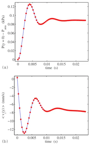
Figure9共a兲shows the temporal evolution of the pressure at the bottom of the cell, i.e., P共y=0,t兲. Figure9共b兲 shows

the averaged vertical velocity of the whole packing,具vy共t兲典 共average of vyfor all the grains兲. Due to the compressibility of the air the pressure is observed to undergo a transient damped oscillation immediately after the cell is rotated. The rotation of the numerical cell is instantaneous, in contrast to the rotation of the experimental cell, and the sudden accel-eration of the grains generates a pressure shock front that propagates into the gap of air. The oscillating pressure causes the averaged vertical velocity of the grains to display a simi-lar oscillation as shown in Fig.9共b兲.

0 10 20 30 40 50 60 70 −0.2 −0.15 −0.1 −0.05 0 0.05 0.1 height (mm) P(y) − P atm (k Pa) t = 0.00 ms t = 0.80 ms t = 1.60 ms t = 2.40 ms 0 10 20 30 40 50 60 70 −0.2 −0.15 −0.1 −0.05 0 0.05 0.1 height (mm) P(y) − P atm (kPa) t = 0.06 s t = 0.12 s t = 0.18 s t = 0.24 s t = 0.30 s (a) (b)

FIG. 7. 共Color online兲 Plots of vertical pressure profiles

aver-aged over the system width.共a兲 Evolution of the pressure

immedi-ately after the cell is rotated.共b兲 The pressure profiles at later times.

The pressure is given as the deviation from 1 atm.

0 10 20 30 40 50 60 70 0 0.1 0.2 0.3 0.4 0.5 0.6 height (mm) ρ (y) t = 0.00 s_{t = 0.06 s} t = 0.12 s t = 0.18 s t = 0.24 s t = 0.30 s

FIG. 8. 共Color online兲 Plot of vertical solid fraction profiles

averaged over the system width. The times of the profiles, except

C. Fourier analysis

1. Solid fraction

In addition to the qualitative comparison of the numerical and experimental data, a quantitative validification is per-formed by means of spatial Fourier power spectra of the solid fraction. By this analysis an average wave number具k典 is obtained which measures the characteristic inverse size of the observed structures.

The average wave number 具k典 is calculated as follows. The power spectrum S共k; j兲 of the solid fraction is calculated by applying the discrete Fourier transform关37兴 on the

hori-zontal lines j of the solid fraction field␳共x,y兲. Here k de-notes the wave numbers of␳共x; j兲, and j is an index running over the horizontal lines of the solid fraction grid. The power spectra S共k; j兲 are further averaged over j to produce a single power spectrum S¯共k兲, representing the state of the system at a given time. The mean具k典 of the averaged power spectrum

S

¯共k兲 is then finally obtained by the common definition of the nth moment

具kn_{典 =}

兺

兺

共5兲 with n = 1. The standard deviation

␴k=

冑

The same analysis is used to extract information about the characteristic size of the experimental structures. The solid fraction is however not directly accessible in the experimen-tal data, and the values of the image pixels, spanning from 0 共black兲 to 255 共white兲, are instead used as an estimate of the real solid fraction. The solid fraction and the pixel value are inverse quantities, i.e., dilute regions have low solid fractions but high pixel values since they appear as white in the im-ages.

The experimental images are 322 pixels in width, whereas the numerical solid fraction grid is only 160 nodes in width. If the mean values of the two power spectra are to be com-parable, the width of the two distributions must be equal. Hence, the experimental power spectrum has an upper cutoff given by the largest wave number in the numerical power spectrum.

The mean, 具k典, and standard deviation, ␴k, of the power spectrum are plotted as functions of time in Figs.10共a兲and

10共b兲, respectively. The data used here are the same as in Fig.4, with an additional data-set from a similar experiment. As the instability evolves the initial discrepancy is reduced, and the consistency of the data for later times is quite good.

0 0.005 0.01 0.015 0.02 0 0.02 0.04 0.06 0.08 0.1 time (s) P( y=0 )−P atm (kPa) 0 0.005 0.01 0.015 0.02 −12 −10 −8 −6 −4 −2 0 time (s) <v i (y) > (mm/s) (a) (b)

FIG. 9.共Color online兲 共a兲 Temporal evolution of the pressure at

the bottom of the cell.共b兲 Vertical velocity of the packing calculated

by averaging over all the grains. Immediately after the cell is flipped a damped oscillation is observed in both pressure and ve-locity, which is a signature of the compressibility of the air.

0 0.1 0.2 0.3 0.4 0.5 0.6 0.7 0 1 2 3 4 time (s) < k > (1/cm) simulation experiment experiment 0 0.1 0.2 0.3 0.4 0.5 0.6 0.7 0 1 2 3 4 time (s) σ k (1/cm) simulation experiment experiment (a) (b)

FIG. 10. 共Color online兲 共a兲 Mean wave number 具k典 of S¯共k兲 as

function of time.共b兲 Standard deviation␴k of S¯共k兲 as function of

time. The results are obtained for two experiments and one

The decrease of␴kin Fig.10共b兲is caused by the increasing length of the fingers: As the fingers grow the amplitude of the wave number associated with the finger separation in-creases, thus reducing the width of the power spectrum dis-tribution.

These results show that our gas-grain system is clearly different from the liquid-grain system discussed by Völtz

et al.关21兴. Their liquid-grain system did not display a wave

number shift with time, nor the cusp-shaped geometry of the fingers.

2. The interface

Instead of analyzing the full solid fraction field␳共x,y兲 for the whole system as in the previous section, the focus is now on the dynamics of the air-grain interface itself.

The function describing the interface is determined by the following procedure. Each vertical line of the solid fraction grid is scanned from top to bottom, and the first node on the line with a solid fraction less than a given threshold is de-fined to be a point on the interface. Together these points define the interface. The value of the threshold is determined by plotting the calculated interfaces on top of the numerical snapshots and visually confirm that they correspond well 共see Fig. 2 of Ref. 关20兴兲. The overall shape of the interface is

not very sensitive to a fine-tuning of the threshold. The

ex-perimental interface is obtained by the same procedure, only with the solid fraction replaced by the image pixel values. The experimental images are rescaled to the size of the nu-merical solid fraction grid before the experimental interface is obtained. The resulting single-valued functions describing the interface at different times are shown in Figs.11共a兲and

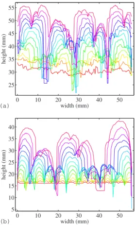
11共b兲 for the experiment and simulation, respectively. The

two series of interfaces have the same temporal separation of 24 ms, and they both start 共bottom兲 at t=0.002 s and stop 共top兲 at t=0.29 s. Salient features of these front evolution plots are the expansion of the bubbles and the appearance of new fingers共shaped like wedges in these plots兲 at the top of the latter interfaces. Comparing Figs. 11共a兲 and 11共b兲, the final shape of the interfaces is in good agreement. The initial shape of the interfaces do not coincide equally well due to the external disturbances introduced in the experimental cell. Figures 12共a兲 and12共b兲 show 共in the same colors as in Fig. 11兲 the power spectrum of every second interface in

Figs.11共a兲and11共b兲, respectively. The location of the maxi-mum wave number for each individual power spectrum is indicated by circles. The numerical power spectra in Fig.

12共b兲 starts out with a maximum wave number to the far right, whereas the experimental power spectra in Fig.12共a兲

starts out with a maximum wave number to the far left. The reason for this discrepant behavior is the very different shape of the initial experimental and numerical interfaces: The

nu-0 10 20 30 40 50 25 30 35 40 45 50 55 width (mm) height (mm) 0 10 20 30 40 50 5 10 15 20 25 30 35 40 width (mm) height (mm) (a) (b)

FIG. 11. 共Color online兲 Temporal evolution of 共a兲 the

experi-mental air-grain interface and共b兲 the numerical air-grain interface.

The interfaces move upward with a temporal separation of 0.024 s. The times of the first and last interface are, respectively, 0.002 and 0.29 s. 1 2 3 4 0 1 2 3 4 5 wave number (1/cm) amplitude t = 0.05 s t = 0.10 s t = 0.15 s t = 0.20 s t = 0.25 s t = 0.30 s 1 2 3 4 0 5 10 15 wave number (1/cm) amplitude t = 0.05 s t = 0.10 s t = 0.15 s t = 0.20 s t = 0.25 s t = 0.30 s (a) (b)

FIG. 12. 共Color online兲 Temporal evolution of 共a兲 the

experi-mental power spectrum and共b兲 the numerical power spectrum. The

power spectrum of every second interface in Fig.11is plotted here.

The times of the power spectra are given in the legend box, and the colored circles indicate the location of the maximum wave number for every time.

merical interface is virtually flat, whereas the experimental interface has noise on all wavelengths. The dominating wave numbers of the latter power spectra in Figs.12共a兲and12共b兲 are only slightly shifted with respect to each other, and con-verge to approximately the same form.

3. Growth rates

We now move on to analyze the growth rates of the wave numbers as they appear in the power spectra of the numerical data. Following the lines of a linear stability analysis we look

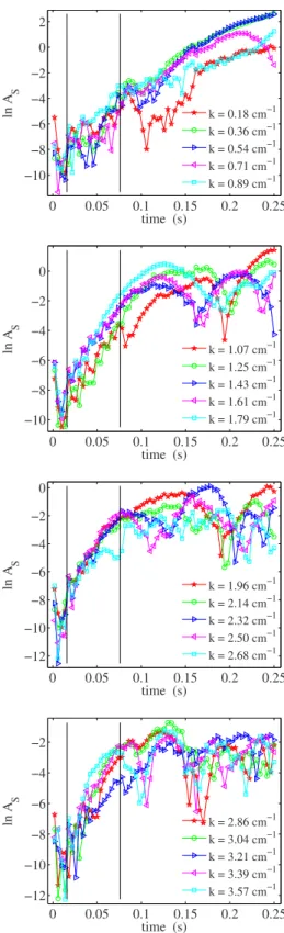
0 0.05 0.1 0.15 0.2 0.25 −10 −8 −6 −4 −2 0 time (s) ln A S k = 0.18 cm−1 k = 0.36 cm−1 k = 0.54 cm−1 k = 0.71 cm−1 k = 0.89 cm−1 0 0.05 0.1 0.15 0.2 0.25 −10 −8 −6 −4 −2 0 time (s) ln A S k = 1.07 cm−1 k = 1.25 cm−1 k = 1.43 cm−1 k = 1.61 cm−1 k = 1.79 cm−1 0 0.05 0.1 0.15 0.2 0.25 −12 −10 −8 −6 −4 −2 0 time (s) ln A S k = 1.96 cm−1 k = 2.14 cm−1 k = 2.32 cm−1 k = 2.50 cm−1 k = 2.68 cm−1 0 0.05 0.1 0.15 0.2 0.25 −12 −10 −8 −6 −4 −2 time (s) ln A S k = 2.86 cm−1 k = 3.04 cm−1 k = 3.21 cm−1 k = 3.39 cm−1 k = 3.57 cm−1

FIG. 13.共Color online兲 Growth rates of the air-grain interface.

The wave numbers are given in the legend boxes, and the vertical lines indicate the time window where the dispersion relation in Fig.

15共a兲is calculated. 0 0.05 0.1 0.15 0.2 0.25 −4 −3 −2 −1 0 1 time (s) ln A S k = 0.18 cm−1 k = 0.36 cm−1 k = 0.54 cm−1 k = 0.71 cm−1 k = 0.89 cm−1 0 0.05 0.1 0.15 0.2 0.25 −4 −3 −2 −1 0 1 2 time (s) ln A S k = 1.07 cm−1 k = 1.25 cm−1 k = 1.43 cm−1 k = 1.61 cm−1 k = 1.79 cm−1 0 0.05 0.1 0.15 0.2 0.25 −4 −3 −2 −1 0 1 time (s) ln A S k = 1.96 cm−1 k = 2.14 cm−1 k = 2.32 cm−1 k = 2.50 cm−1 k = 2.68 cm−1 0 0.05 0.1 0.15 0.2 0.25 −4 −3 −2 −1 0 time (s) ln A S k = 2.86 cm−1 k = 3.04 cm−1 k = 3.21 cm−1 k = 3.39 cm−1 k = 3.57 cm−1

FIG. 14. 共Color online兲 Growth rates of the bulk solid fraction.

The wave numbers are given in the legend boxes, and the vertical lines indicate the time window where the dispersion relation in Fig.

for possible early exponential growth of the wave numbers in the power spectrum of both the air-grain interface profile and the full solid fraction field.

The temporal evolution of the 20 smallest wave numbers in the power spectrum共or equivalently the 20 longest wave-lengths兲 of the interface profile are plotted semilogarithmi-cally in Fig. 13. The corresponding plots for the average power spectrum of the solid fraction field, S¯共k兲, are shown in Fig.14. Exponentially growing wave numbers will appear as linear in these plots. The growth of the solid fraction wave numbers in Fig.14is less noisy compared to the growth of the interface wave numbers in Fig.13due to the averaging of the solid fraction power spectrum S¯共k兲 共see IV C 1兲.

Judging by the growth rates shown in Figs.13and14it seems fair to conclude that none of the wave numbers follow an exponential growth共at least not of any significant dura-tion兲. Hence, the granular Rayleigh-Taylor instability is in-herently nonlinear, in contrast to the classical Rayleigh-Taylor instability. Nevertheless, a linear least squares fit is obtained for all the wave numbers of the power spectrum, including those not displayed in Figs.13 and14. The fit is performed over a time window of 0.6 s as indicated in the plots. The resulting growth rates␣I共interface兲 and␣S 共solid fraction兲 as functions of wave number k are shown in Figs.

15共a兲and15共b兲, respectively. In these figures each data point is a box average over eight wave numbers. The standard deviation is indicated by the error bars. Given the approxi-mate linearity of the wave number growth, vigorous

conclu-sions cannot be drawn from these plots. However, while our measurements do not serve to identify a well defined window of linear growth, the growth rates nevertheless exhibit the dominating, time dependent wave number: The maxima at ⬃4 cm−1 _{in Figs. 15共a兲 and 15共b兲 coincide with the t} = 0.05 s maximum of the power spectrum in Fig. 12共b兲. However, it is clear that nonlinear mechanisms govern the selection of the final dominating wavelength.

In a well-controlled experiment of the classical Rayleigh-Taylor instability it is possible to observe exponential growth over a time sufficiently long to erase the influence of the initial noise. This is not the case, however, for the granular Rayleigh-Taylor instability since the exponential domain of the wave number growth is too short to cancel the initial noise. Hence, the structures that develop early, i.e., on a time scale of about 0.1 s, are sensitive to the initial structure of the system. Note that this initial structure is not an experi-mental imperfection but an intrinsic, unavoidable feature of granular packings.

D. Changing simulation parameters

A number of simulations are performed to probe the re-sponse of the instability as the input parameters are changed, i.e., the density of the grains, the roughness of the initial interface, and the dissipation of the granular phase.

1. Grain density

A comparison of simulations performed using grains of different densities, but with identical start configurations, is presented. The density of the grains is 1.05 g/cm3 共polysty-rene兲 or 2.5 g/cm3_{共glass兲, and the diameter is 140␮m.}

Fig-ures16共a兲 and16共b兲 show plots of the mean wave number

具k典 and the standard deviation␴kof the power spectrum S¯共k兲 as functions of time. From these plots it is observed that the time of breakthrough, i.e., when the bubbles reach the upper surface, is dependent on the density of the grains. The sepa-ration in time between the last data points of each curve in Fig.16共a兲shows that the instability develops faster if heavier beads are used. However, the initial decrease 共i.e., from t = 0 to 0.1 s兲 of 具k典 and␴kare roughly the same for the two densities.

2. Initial interface

The response of the instability to different initial air-grain interfaces is investigated by three simulations using inter-faces with a variation in the roughness.

The three interfaces, shown in Fig. 18 where they are denoted A, B, and C in increasing order of roughness, are prepared as follows. Starting from a configuration where the packing rests on the bottom plate, interface A is created by displacing the packing vertically upward to fill the top half of the cell. In this case the cell is not rotated. A perfectly flat air-grain interface is now defined by the grains originally positioned on the bottom plate, prior to the vertical displace-ment. Interface B is created by first removing all grains with their centers above a given height just below the upper sur-face of the packing 共again positioned on the bottom plate兲.

2 4 6 8 10 12 20 40 60 80 100 120 wave number, k (1/cm) growth rate, α I (1/s) 2 4 6 8 10 12 20 30 40 50 60 70 80 wave number, k (1/cm) growth rate, α S (1/s) (a) (b)

FIG. 15. 共Color online兲 Dispersion relation 共a兲 of the air-grain

interface and共b兲 for the bulk solid fraction. The relations are

ob-tained by linear fits over the approximate linear parts of the growth

rate plots in Figs.13 共interface兲 and15 共bulk solid fraction兲. The

The cell is then rotated to bring the slightly rough surface above the layer of air. Interface C is the rotated original packing with a surface determined by the local equilibrium of the grains.

The temporal evolution of具k典 and ␴kfor packings with their initial interfaces as shown in Fig.18are plotted in Figs.

17共a兲and17共b兲, respectively. These plots lead to the conclu-sion that the shape of the initial interface has an effect only during the earliest stages of the instability. It appears that the slowest evolving interface is B, and that B, not A, is the interface with the smallest initial noise. This may correspond to the fact that the porosity above interface A has larger fluctuations than in B because of the constraint imposed by the flat wall. After about 0.2 s the difference in具k典 is negli-gible. The increased standard deviation of interface A indi-cates a slightly slower and delayed generation of fingers in this case. However, the effect is only temporary and the ini-tial difference is canceled out. Note that this observation is consistent with the conclusion at the end of Sec. IV C 3: The exponential domain is too short to cancel the initial noise during the incipient evolution of the instability. However, as nonlinear effects take over, the system nevertheless evolves toward structures that are insensitive to the initial noise.

3. Dissipation

A series of simulations are performed where the coeffi-cient of normal restitution,␧, is changed. The motivation is to investigate the effect on the fingering process and its

dy-namics. Figure19 shows two snapshots for each of the six different restitution coefficient used in these simulations. The two leftmost snapshots in Fig.19, with␧=1.0 and 0.95, dis-tinguish themselves by a diffuse outline of the interface, fewer fingers, and a general lack of detail compared to the other snapshots. To differentiate between the remaining pairs of snapshots, obtained with␧=0.8, 0.5, 0.2, and 0.05, is not as evident because it is difficult to identify significant differ-ences in these images: The number of fingers is about the same, as well as the size and shape of the bubbles. It is possible to identify minor deviations in, e.g., the number and shape of the renucleated fingers, but no significant influence of dissipation is observed on the formation of new fingers. The conclusion must be that the system is invariant under changes in the dissipation as long as the restitution coeffi-cient is below a certain threshold. However, above this threshold the instability is sensitive to variations in the res-titution, in particular the size and shape of the fingers are affected. The curvature of the bubbles is only moderately affected by the variation in␧.

The value of the threshold, above which the instability is virtually insensitive to variations in␧, is likely to depend on

0 0.1 0.2 0.3 0.4 0.5 0.6 0.7 0 1 2 3 4 time (s) < k > (1/cm) ρ_g= 1.05 g/cm (polystyrene) ρ_g= 2.50 g/cm3(glass) 0 0.1 0.2 0.3 0.4 0.5 0.6 0.7 0 1 2 3 4 time (s) σ k (1/cm) ρ_g= 1.05 g/cm3(polystyrene) ρ_g= 2.50 g/cm3(glass) (a) (b)

FIG. 16.共Color online兲 共a兲 Mean wave number 具k典 as a function

of time for different grain densities.共b兲 Standard deviation␴kas a

function of time for different grain densities. The grain densities␳_g

used in the simulations are given in the legend box.

0 0.05 0.1 0.15 0.2 0 1 2 3 4 5 time (s) < k > (1/cm) interface A interface B interface C 0 0.05 0.1 0.15 0.2 0 1 2 3 4 time (s) σk (1/cm) interface A interface B interface C (a) (b)

FIG. 17.共Color online兲 共a兲 Mean wave number 具k典 as function

of time for different initial interfaces.共b兲 Standard deviation␴_kas

function of time for different initial interfaces. The interfaces used

in the simulations are labeled A, B, and C and are shown in Fig.18.

C A B

FIG. 18. Different initial air-grain interfaces used in the simula-tions. The interfaces are labeled A, B, and C in increasing order of roughness.

the average number of collisions the grains participate in. The number of collisions n required to reduce the kinetic energy by a given fraction F is inversely proportional to the logarithm of the restitution coefficient ␧. In mathematical terms n共␧兲=ln共1−F兲/ln共␧兲 which follows from the relation ␧n_{= 1 − F. A semilogarithmic plot of n共␧兲 for three different} values of F is shown in Fig.20. Lets assume a grain has lost 90% of its kinetic energy by interacting in n

⬘

⬘

⬘

⬘

demonstrates that the number of collisions needed to reduce the energy by, e.g., 90% changes significantly as the restitu-tion coefficient changes from 0.99共229 collisions兲 to 0.8 共ten collisions兲. Below this interval the change in the number of collisions is marginal: At ␧=0.6 it takes five collisions to

reduce the energy by 90%, compared to ten collisions at ␧ = 0.8. If we assume that a grain on average is involved in ten collisions, over a time scale that is small compared to the dynamical time scale of the structures, 90% of its energy is lost if␧=0.8, and 99% is lost if ␧=0.6. Since most of the energy is already dissipated at␧=0.8, this might explain why the simulations are virtually invariant if the restitution coef-ficient is reduced beyond␧=0.8.

V. CONCLUSION

A gravitational instability, observed as a layer of dense granular material is positioned above a layer of air in a closed Hele-Shaw cell, is reported both experimentally and numerically. Qualitative and quantitative comparisons of nu-merical and experimental data are presented with the conclu-sion that the simulations reproduce the essential experimen-tal features. The growth rates of the numerical solid fraction field are obtained by Fourier analysis to look for exponential time dependence. Both the bulk solid fraction and the air-grain interface have been investigated by this analysis. Our conclusion is that granular Rayleigh-Taylor instability is in-herently nonlinear since exponential dependence of signifi-cant duration is not observed in the data. Further, the re-sponse to changes in different simulation parameters was probed: The density of the grains, the initial air-grain inter-face, and the granular dissipation. Increasing the density leads to an earlier breakthrough of the air bubbles, without any significant change in the coarsening time of the struc-tures. Changing the roughness of the initial interface has an effect only early in the instability; the difference is canceled after about 0.2 s. Dissipation affects only the formation of fingers above a certain threshold of the restitution coefficient.

t = 0 .125 s t = 0 .250 s ε = 1.0 ε = 0.95 ε = 0.80 ε = 0.50 ε = 0.20 ε = 0.050

FIG. 19. Snapshots of simulations with different coefficients of restitution␧, given below the snapshots. The times of the simultaneous

snapshots are given to the left of each row.

0 0.2 0.4 0.6 0.8 1 1 10 50 100 500 restitution coefficient, ε num ber of co lli si ons, n F = 99.9 % F = 99.0 % F = 90.0 %

FIG. 20.共Color online兲 Number of collisions n as a function of

restitution coefficient␧ 共normal兲. The three different curves show

how many collisions it takes to reduce the kinetic energy of a grain

granular kinetic energy.

The unique behavior of the gas-grain system as compared to the liquid-grain system investigated by Völtz et al. might be caused by the compressibility and low inertia of the air.

As for the experimental work, some refinements of the experiment is necessary if the complete evolution of the in-stability, including the initial fingers, is to be probed.

The work was supported by NFR, the Norwegian Research Council. A special thanks to Sean McNamara for useful comments, and for making the original F90 imple-mentation of the gas-grain model available during theC⫹⫹

reimplementation.

关1兴 Physics of Dry Granular Media, edited by H. J. Herrmann J.-P. Hovi, and S. Luding, NATO Advanced Study Institute, Series

E: Applied Sciences共Kluwer Academic Publishers, Dordrecht,

1998兲, Vol. 350.

关2兴 J. F. Davidson and D. Harrison, Fluidization 共Academic Press,

New York, 1971兲.

关3兴 D. Gidaspow, Multiphase Flow and Fluidization 共Academic

Press, San Diego, 1994兲.

关4兴 G. K. Batchelor, J. Fluid Mech. 52, 245 共1972兲.

关5兴 J. F. Richardson and W. N. Zaki, Trans. Inst. Chem. Eng. 3, 65 共1954兲.

关6兴 P. Y. Julien, River Mechanics 共Cambridge University Press,

Cambridge, U.K., 2002兲.

关7兴 D. H. Rothman, J. P. Grotzinger, and P. B. Flemings, J.

Sedi-ment Res. 64, 59共1994兲.

关8兴 R. Bachrach, A. Nur, and A. Agnon, J. Geophys. Res. 106,

13515共2001兲.

关9兴 P. G. Drazin and W. H. Reid, Hydrodynamic Stability

共Cam-bridge University Press, Cam共Cam-bridge, U.K., 1981兲.

关10兴 S. Chandrasekhar, Hydrodynamic and Hydromagnetic Stability 共Dover Publications, New York, 1981兲.

关11兴 P. G. Saffman and G. Taylor, Proc. R. Soc. London, Ser. A 245, 312共1958兲.

关12兴 C. Chevalier, M. B. Amar, D. Bonn, and A. Lindner, J. Fluid

Mech. 552, 83共2006兲.

关13兴 Ø. Johnsen, R. Toussaint, K. J. Måløy, and E. G. Flekkøy,

Phys. Rev. E 74, 011301共2006兲.

关14兴 G. I. Taylor, Proc. R. Soc. London, Ser. A 132, 499 共1931兲. 关15兴 M. P. Ciamarra, A. Coniglio, and M. Nicodemi, J. Phys.:

Con-dens. Matter 17, 2549共2005兲.

关16兴 J. J. Wylie, Q. Zhang, and X. Sun, Phys. Rev. Lett. 97, 104501 共2006兲.

关17兴 F. Malloggi, J. Lanuza, B. Andreotti, and E. Clement,

Euro-phys. Lett. 75, 825共2006兲.

关18兴 D. Gendron, H. Troadec, K. J. Måløy, and E. G. Flekkøy,

Phys. Rev. E 64, 021509共2001兲.

关19兴 E. G. Flekkøy, S. McNamara, K. J. Måløy, and D. Gendron,

Phys. Rev. Lett. 87, 134302共2001兲.

关20兴 J. L. Vinningland, Ø. Johnsen, E. G. Flekkøy, R. Toussaint,

and K. J. Måløy, Phys. Rev. Lett. 99, 048001共2007兲.

关21兴 C. Völtz, W. Pesch, and I. Rehberg, Phys. Rev. E 65, 011404 共2001兲.

关22兴 G. Taylor, Proc. R. Soc. London, Ser. A 201, 192 共1950兲. 关23兴 R. Jackson, The Dynamics of Fluidized Particles 共Cambridge

University Press, Cambridge, U.K., 2000兲.

关24兴 S. Schwarzer, Phys. Rev. E 52, 6461 共1995兲.

关25兴 S. McNamara, E. G. Flekkøy, and K. J. Måløy, Phys. Rev. E 61, 4054共2000兲.

关26兴 D.-V. Anghel, M. Strauss, S. McNamara, E. G. Flekkøy, and

K. J. Måløy, Phys. Rev. E 74, 029906共E兲 共2006兲.

关27兴 H. Darcy, Les Fontaines Publiques de la Ville de Dijon

共Dal-mont, Paris, 1856兲.

关28兴 P. C. Carman, Trans. Inst. Chem. Eng. 15, 150 共1937兲. 关29兴 F. Radjai, M. Jean, J.-J. Moreau, and S. Roux, Phys. Rev. Lett.

77, 274共1996兲.

关30兴 L. Brendel and S. Dippel, Physics of Dry Granular Media 共Kluwer Academic, Dordrecht, 1998兲.

关31兴 M. P. Allen and D. J. Tildesley, Computer Simulation of

Liq-uids共Clarendon Press, Oxford, 1989兲.

关32兴 J. J. Moreau, Eur. J. Mech. A/Solids 13, 93 共1994兲.

关33兴 M. Jean, in Mechanics of Geometrical Interfaces, edited by A.

P. S. Selvadurai and M. J. Boulon共Elsevier Sciencs,

Amster-dam, 1995兲, pp. 463–486.

关34兴 F. Radjai and S. Roux, Phys. Rev. E 51, 6177 共1995兲. 关35兴 A. Hurst, J. Cartwright, M. Huuse, R. Jonk, A. Schwab, D.

Duranti, and B. Cronin, Geofluids 3, 263共2003兲.

关36兴 H. A. Janssen, Z. Vereines Deutsch. Ingenieure 39, 1045 共1895兲.

关37兴 W. H. Press, S. A. Teukolsky, W. T. Vetterling, and B. P.

Flan-nery, Numerical Recipes in C⫹⫹ 共Cambridge University