HAL Id: insu-02155799
https://hal-insu.archives-ouvertes.fr/insu-02155799
Submitted on 30 Jul 2020HAL is a multi-disciplinary open access
archive for the deposit and dissemination of sci-entific research documents, whether they are pub-lished or not. The documents may come from teaching and research institutions in France or abroad, or from public or private research centers.
L’archive ouverte pluridisciplinaire HAL, est destinée au dépôt et à la diffusion de documents scientifiques de niveau recherche, publiés ou non, émanant des établissements d’enseignement et de recherche français ou étrangers, des laboratoires publics ou privés.
The geomagnetic variation anomaly in the northern
Pyrenees: study of the temporal variation
G. Vasseur, K. Babour, Michel Menvielle, Jean-Claude Rossignol
To cite this version:
G. Vasseur, K. Babour, Michel Menvielle, Jean-Claude Rossignol. The geomagnetic variation anomaly in the northern Pyrenees: study of the temporal variation. Geophysical Journal International, Ox-ford University Press (OUP), 1977, 49 (3), pp.593-607. �10.1111/j.1365-246X.1977.tb01306.x�. �insu-02155799�
Geophys. J. R . astr. SOC. (1977) 49,593-607
The geomagnetic variation anomaly
in
the northern
Pyrenees: study of the temporal variation
G.
VasseUr
Centre Gdologique et Gdophysique - USTL, Place E'Bataillon, 34060 Montpellier Cedex, FranceK. Bab our
Centre de Recherches Gdophysiques, Laboratoire de Gdomagndtisme. 24, rue Lhomond, 75231 Pans Cedex 0 5 , FranceM.
Menvielle and J.
c.
Rossignol
Institur de Physique du Globe, 4 , Place Jussieu, 75230 Paris Cedex 05. FranceReceived 1976 October 29; in original form 1976 July 14
Summary. The existence and the spatial properties of an important geo- magnetic anomaly in the north of the eastern part of the Pyrenees have been described in a previous paper of this journal (Babour et
d.).
The temporal dependance of the anomalous magnetic field and its relation with the normal field is now studied. Due to its remarkable property - separation of spatial and temporal variations - only one component of the anomalous field at one station needs to be considered. A high coherency between the variations of the anomalous field and those of the normal field projected in the direction40"E of north is found. Transfer functions are obtained in the frequency
domain and also directly in the time domain using two different methods. The various estimates of the transfer function are in good agreement for the period range 20min-2hr.
As
the anomaly is due to a concentration of currents induced elsewhere, the obtained transfer function is interpreted in terms of a non-local relation associated with the area where the induction takes place which is identified with oceanic regions. Using reasonable assump- tions, the transfer function is shown to be connected to the ratio of the elec- tric to magnetic field over oceanic areas. The existence of a highly conducting medium at 50 km depth is proposed. The mechanism responsible for the con- centration of currents is qualitatively discussed in relation with the geometry of continental margins.1 Introduction
1.1 S U M M A R Y O F P R E V I O U S R E S U L T S
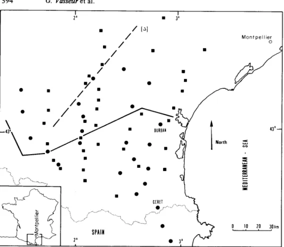
In a previous paper (Babour et d. 1976), we have presented the results of a set of geo- magnetic experiments carried out in the north of the eastern part of the Pyrenees (Fig. 1). In
594 G. Vasseur et al. I I 2'
.
3' / 131 Montpel Iier 0/
. /
/
./
/ O..
-
4 w L az Y wc
. . . ...=
0 Y\
-43' 0 "! ... . . . . . . CI z C!RtI.
... ... . . . ... .... .... . . . .... _. ... 0 0 I0 20 30Lm SPAIN 2' 0 3'Figure 1. Location of the stations occupied from 1972 to 1975 in the eastern part of the northern Pyrenees. The full broken line represents the trend of the geomagnetic anomaly and the dashed line (A)
is the direction most effective for induction. Round: Mosnier variometers; square: Askania.
the studied area, a geomagnetic anomaly has been found by investigating the differences between the time variations of the field recorded in the various stations and the time varia- tions of the field simultaneously recorded in a reference station. As discussed in the previous paper, this reference station - Ceret (Fig. 1) - is considered as a normal one since it is
located in an area where the horizontal field has been found homogeneous. Therefore the differences of the horizontal field are identified with the horizontal components of the anomalous field. This geomagnetic anomaly whose trend is sketched on Fig. 1 is a very strong one: the variations of the horizontal anomalous field Ha(t) and those of the normal field can have comparable amplitudes in the vicinity of the maximum of the anomaly. Furthermore, it has been pointed out (Babour et ul. 1976) that the anomaly has a fixed
geometry independent of the period for magnetic variations of period greater than 10min. This property is valid for any type and any amplitude of disturbance; it implies that the anomalous field is the product of a function of time R ( t ) by a function of space h,(P)
H,(P, t ) = h,(P) . R ( t ) . (1)
This property has been checked in the time domain by the similarity which exists between any two components ( @ ( t ) and \k(t)) of the anomalous field observed simulta-
neously either in two different stations or in the same station. In the frequency domain,
Geomagnetic variation anomaly 595 this property implies a linear relationship between the Fourier components of @(t) and
\k(t). This can be shown by studying the coherency between @ ( t ) and 9 ( t ) defined by
SoQ and S,p, being the power spectrum of @ and 9 respectively, S,, being their cross spectrum. For all the cases, C ( f ) is greater than 0.92 for periods over 600s and the imagi-
nary part of S@, is less than 1 per cent of the real part. These two properties prove, in the frequency domain, that the components @ and 9 are proportional.
The character of the electric currents responsible for the anomaly was previously dis- cussed (Babour et al. 1976). The large amplitude of the anomalous field and its property
(equation 1) imply that these currents are not locally induced in some elongated conducting structure; instead of that, the anomaly is due to currents induced in large surrounding areas and locally channelled. Therefore the function R ( t ) must be linearly related to the normal
field in the area where these currents are induced.
1.2 P U R P O S E O F T H E P R E S E N T W O R K
The previous paper dealt with the study of the spatial dependence of the anomalous field -
h,(P). The purpose of this paper is to study the relation between the time variations of the anomalous field R ( t ) and those of the normal field, using various methods.
At mid-latitude and for the magnetic events that we have studied - bay type variations - the external field can be considered as uniform over horizontal distances of several hundred kilometres (Rikitake 1966); the vertical component of the normal field is then small compared to it.s horizontal components. Therefore, it can be assumed that the variations of the normal field in the area where induction occurs and those of the normal field near the anomaly are identical, although the location of the area where induction occurs is largely unknown. Thus a relationship between the variations of the anomalous field and those of the normal field simultaneously recorded outside the anomaly should be studied.
The approach which is the most commonly used for the study of geomagnetic anomalies, is the computation in the frequency domain of transfer functions between the variations of
the vertical component Z of the geomagnetic field and those of the horizontal component
of the normal geomagnetic field. Thus, it is assumed that the vertical component Z in the anomalous area is entirely anomalous - or at least that its normal part does not correlate
with the normal horizontal field. For the present study, the experimental method used (Babour & Mosnier 1976), provides - with a good accuracy - the horizontal component
of the anomalous field. Furthermore, the relation (1) allows one to compare the variations
of one component of the anomalous field - R ( t ) - recorded in one station to the simulta-
neous variations of the field H,(t) recorded at the reference station assumed to be a normal
one.
We have chosen for R ( t ) the north-south component of the anomalous field at the
Durban station (cf: Fig. 1) - located near the maximum of the anomaly - and for H,(t), the
field recorded at the Ceret station as discussed in the first paragraph. We have selected three samples during which large variations of the field occur - several tens of gammas on the normal field - and without preferential direction of polarization. The characteristics of these events are described in Table 1 .
These three events have been used to look for the relationship between the variations of the anomalous field R(t) and those of the normal horizontal field H,(t). This relationship
will be first studied in the frequency domain and then in the time domain. The results will be compared and interpreted.
596 G. Vusseur et al. Table 1. No. Beginning 1 1973 Oct. 5 1 8 h L.T. 2 1975 Oct. 8 18 h L.T. 3 1974 Oct. 17 18 h L.T. End Oct. 6 02 h L.T. Oct. 9 06 h L.T. Oct. 18 02 h L.T. 2 Analysis in the frequency domain
2.1 S P E C T R A L E S T I M A T E S
In order to obtain a good estimate of the power spectra for periods less than 1 or 2 hr, the
data were filtered using a high pass filter with a cut-off period of 7200 s. The filters used are
Butterworth recursive filters (Souriau 1974); they provide an attenuation of 0.5 for the
cut-off period and an attenuation rate of 36 dB/octave. The auto- and cross-covariance functions were then computed and multiplied by a Parzen window of half-width 3000s (Jenkins & Watts 1968). Finally, taking the Fourier transform of these functions, we have
obtained an estimate of the spectra with a frequency interval of 1.67 x Hz.
Cohsrancy
t
A
fl
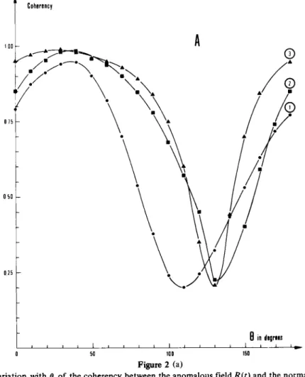
in dipriis 1 , , 1 1 , , , 1 , , 1 1 1 , - ~ 0 50 100 I50 Figure 2 (a)Figure 2. Variation with 0 of the coherency between the anomalous field R ( t ) and the normal horizontal field projected upon the direction e : Hn, (t) = Hn cos 0 + D n sin 0 (0" 4 0 Q 180"). Cases A, B, C corre- spond to samples 1, 2 and 3; on each figure the following period bands are considered: 1 - period band 2000-6000 s; 2 - period band 1200-2000s; 3 - period band 900-1200s.
Geomagnetic variation anomaly 597 Coherency
t
1 0 0t
B
2.2 D I R E C T I O N MOST E F F E C T I V E F O R I N D U C T I O NTo find the direction most effective for induction, i.e. the direction (A) along which the coherency between the normal and the anomalous field is maximum, the coherency - defined by (2) - between R ( t ) and the normal horizontal field projected on the direction of
the unit vector has been computed (Fig. 2). 8 is the angle between the magnetic north and u, positive to the east. An obvious maximum of coherency - greater than 0,82 for all the samples and for all the period range under study - occurs around 8 = 40"E of north. Thus the direction 40"E of north is the one where induction is most effective for the observed anomaly.
In addition, the cross spectrum between R ( t ) and Hn,40o(t) has an imaginary part which is
relatively large compared to its real part, i.e. there is a phase shift between R ( t ) and
Hn, 40° ( t ).
2.3 T R A N S F E R F U N C T I O N S
Let
&f)
and&f)
be the Fourier transforms of the north-south and east-west com- ponents of the normal horizontal field H,(t) and &f) that of R(t). The real coefficientsa&), b~(f). a~(f), b ~ ( f ) of the transfer function are those which minimize the residual
598 G. Vusseur et al. Cohsrsncy
t
c
B
in dalros 0i
50 100 150 Figure 2 (c) (3) power l6kI'
in the following equationk
= ( a H t i b H )2
t (a0 t i b D )d
t 6R".This transfer function is usually characterized (Schmucker 1970; Cochrane & Hyndman 1970) by the in-phase vector A(f) and the out-of-phase vector B(f) whose components are respectively ( - a H , - u D ) , ( b H , b ~ ) . Fig. 3 shows the modulus of the vectors as well as their direction with respect to the magnetic north - these directions being positive toward the east. The directions of vectors A and B obtained with the three samples are in reasonable agreement; moreover, the vectors A and B have roughly the same direction: 40°E of north. This result expresses in a different way the previous result (Fig. 2). The moduli IAI and IBI are also comparable among individual samples. For period less than 900 s, IA
I
is greater than 1, i.e. the anomalous field considered is greater than the normal one. The ratio IAI/IB/ varies from 0.25 to 0.5 when the period varies from 600 to 5400s; so the phase shift between normal and anomalous field increases with the period.3 Analysis in the time domain
The study of the relationship between the anomalous field and the normal one is now carried out directly in the time domain; this study can be started in, mainly because of the characteristics of the experimental equipment which allows to obtain the various fields with
501
* t* 0 '* 30cf
iniLf
In HZ 0- 1 L i. i I 1 , 1 5x10 10.10 15x10' 17x10 5x10 ' 10.10 15x10 17x10 '4
liil 3 5-.
r* ._ 0- I 20 mn .* .* .* 0 0 0 I IOmn 0 0 *+4"r
L.30t
'0 b 5x10.' 1+ 2. 3,I
mn 0I
lo"<? - 0 0 00f
In IIZ L- -- -Ldy- 10x10 ' 15x10.' 17x10 Fi 3. On the left part: modulus of the in phase IAl and out of phase IBI induction vectors as a function of frequency for three samples. On the right part: direction in degree of the vectors A and B with respect to the magnetic north (positive to the east).600 G. Vasseur et al.
a good accuracy: differences measured in real time with high stability and low noise sensors (Babour & Mosnier 1976). Therefore the impulse response of the convolution filter which transforms the normal field H,(t) into the anomalous one R ( t ) has been calculated.
This
filter is equivalent in the time domain to the transfer function in the frequency. domain. The impulse response of this linear filter has been found out by two different ways: (i) using the discrete Wiener filter formulation; (ii) assuming that the behaviour of the linear filter which yields R ( t ) from H,(t), may be described by a linear differential equation and by computing
the coefficients of this equation.
3.1 D E T E R M I N A T I O N O F T H E W I E N E R F I L T E R
Let X ( t ) be the projection of H,(t) on the direction (A) most effective for induction (40' E
of north, cf: Section 2). R ( t ) is supposed to be linearly related to
x(t)
byR ( t ) =
J'-
h(u) X ( t - u ) du+
6 R ( t ) 0(4)
where h(t) is the impulse response of the linear filter assumed to be physically realizable
(i.e. its impulse response is causal: h(t) = 0 when t < 0) and 6R(t) is a residual. Minimizing the average power of this residual leads to the well known Wiener-Hopf integral equation
where yxx(r) and T X R ( r ) are respectively the autocovariance and cross covariance functions
of X ( t ) and R(t). For discrete time series ( t = nT where n is an integer-valued index and T
the sample rate), the discrete operator (h,, n = 1 , 2 ,
.
. .
, N ) corresponding to h(t) mustsatisfy a system of equations (Treitel & Robinson 1966)
N
1
h,cnm=d,, m = 0 , 1 ,...,
Mn = O
with c,, = 7xx(n - m ) T and d , = y x R ( m T ) M t 1 is the number of equations considered.
The number of coefficients h, is arbitrarily limited to N t 1 non-zero values. Let C be the matrix [c,,], d and h the vectors [d,] and [ h , ] . In the case M > N , the system (6) is over- constrained; it can be solved using least-square techniques, i.e. by minimizing the value of
IIC ah - dll. However, the solution obtained presents large oscillations; this instability is due
to the bad conditioning of the matrix C. It is possible to eliminate this instability by intro- ducing an approximate solution ho and by minimizing IIC* h - dll t Allh - hO1l, where h is
a positive parameter. The greater A is chosen, the smaller Ilh -
boll
will be. In fact, a verysmall value of A - less than 1/100 of the diagonal elements of C - is enough to obtain a
stable solution. For the value of ho, a simple proportionality between X ( t ) and R ( t ) was chosen, using the similarity between these two time series (this similarity can be noticed on Fig. 5). Tests have indicated that the resulting solution h is relatively independent of the choice of ho.
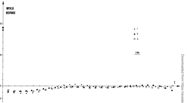
Fig. 4 gives the impulse responses obtained for the three samples with T - 120 s , M = 35
and N = 30 (maximum delay 3 60 mn): the three curves are very close one to another.
Using the arithmetic average of these three estimates, a mean impulse response can be calculated. In order to obtain a predicted output R'(t) and to compare it to the actual series
R(t), the input
x(t)
is convolved with thls mean impulse response. An example of this com-Geomagnetic variation anomaly 60 1 IYPULSf RfSPOWSt 1.0
1
r l A 2 0 3 I tFigure 4. Impulse response of the discrete Wiener filter obtained with the three samples 1, 2 and 3 as a function of the delay.
parison is shown on Fig. 5 and shows a good agreement, except for a discrepancy for the hghest frequencies.
3.2 C O M P U T A T I O N O F T H E C O E F F I C I E N T S O F A D I F F E R E N T I A L E Q U A T I O N
Another direction of investigation is to estimate a simple dynamic model equivalent to the linear system relating the anomalous field to the normal one. We may assume that the system is governed by the simple differential equation, similar to the equation for the intensity in a resistance-inductance circuit:
where 7 is an unknown time constant and S(t) a linear function of the input Hn(t). The
induction laws suggest that S ( t ) = dCP/dt with CP = v.H,,(t), v being an horizontal vector
whose components are OL and
0.
As €3, ( t ) and R ( t ) are digitized with a sample rate T , r , OL and
/3
must verify the followingsystem 27
+
T OL 2 7 - T 2 ~ - T R [ ( n - 1 ) TI =-
R(nT) t-
[H[(n - 1) TI - W T ) I [" - 1 ) TI - a n 7 3 1 (8)P
2 ~ - T t-for n = 1 , 2,
. . .
, N, N being the number of points of the observed time series. The system (8)is obtained by taking the z transform of (7) -the operator d/dt being estimated by
( 2 / T ) [(I - z ) / ( l t z)l *
c
OC!.
8,1975 OL!. 9,1975 Figure 5. Example of reconvolution of the normal horizontal field projected on the direction 40" E of north with the average impulse response deduced from Fig. 4. From top to bottom: A - projected normal field Hn,400(t); B - continuous line is the observed anoma- lous field R(f); dashed line is the predicted anomalous field R'(r); C - difference between the predicted and the measured anomalous field R'(t) -R(r).Geomagnetic variation anomaly 603 In practice, R ( t ) is only known to within a weak additive constant (Babour & Mosnier
1976); however, in equation (7), the actual value of R ( t ) is assumed to be known. So, we
have to introduce, for every sample, the average value of R(r) as an additional unknown
parameter in (8).
This
system is then solved using least-square techniques. The value of is the time constant of the system governed by (7), tan-'(alp)
gives the direction most effec- tive for induction (A), (az+
f12)''2/~
is the magnification factor of the dynamic system.the time series have been previously filtered using linear Butterworth filters described above. The results are independent of the sampling interval T. Table 2 gives the results for the three samples in the period range 1200-
5400 s.
For the computation of the parameters 7 , a,
Table 2.
No. TS (a' + p*)"'s e = tan-' @/a)
1 14 1 666 40"
2 193 I55 3 3"
3 116 112 3 9"
The values obtained for parameters T , a, are in good agreement. The direction
8 = tan-' (p/a) is very close to the direction found previously. Solving equation (7)
with
mean values of parameters ( 7 = 775 s, (a2 t
p2)'''
= 736 s, 8 = 37") a predicted output R'(t)can be obtained and compared to the actual R ( t ) series (Fig. 6). The agreement between R ( t ) and R'(t) is very good.
4 Comparison of the estimated transfer functions
The validity of the results obtained in the time domain has been verified through the com- parison between the observed time series R ( t ) and the predicted ones. From these results,
two estimates of the transfer function between R ( t ) and the projected normal field have
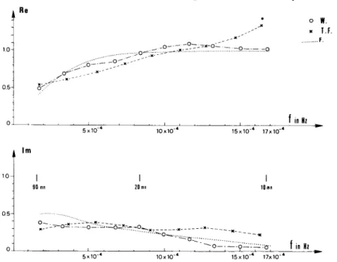
also been obtained. These two estimates are compared to the previous one obtained in the frequency domain. Fig. 7 shows the estimated transfer functions (real and imaginary parts) obtained using these three methods:
(i) TF, obtained through the spectral analysis, is the arithmetic average of the curves of Fig.
3 corresponding to the three samples;
(ii)
W ,
is the Fourier transform of the average impulse response deduced from Fig.4;
(iii) F , arises from the functional relation (7). Its analytical expression is
F ( f ) = (az t pz)'"(2h .f)/(l t 2 b .f~). ( 9 )
Mean values of parameters 7 , a,
p
have been used.The agreement between the three curves is quite good both for real and imaginary parts. However, for shorter periods (less than about 800 s), a discrepancy can be noted and can be explained by the following remarks:
(i) for this frequency range, the spectral power is low and the spectral estimates may be erroneous;
(ii) the Fourier transform of the impulse response of Fig. 4 is not accurate for higher
frequency ;
(iii) the curve labelled F was obtained with filtered data using a band pass filter attenuating high-frequency components.
Nevertheless, for periods less than 1200 s the differences between the three estimated real parts of the transfer function are about 10 per cent and reach at most 30 per cent for
\ t o/.;
;^.
:-
?.-.
19h ‘w‘
T
Oct. 11.1974 Oct. 18.1914
Figure6. Comparison of the observed anomalous field R ( t ) (continuous line) with the predicted anomalous field R‘(r) (dashed line) obtained through integration of equation (7) with T = 775 s,
(a’ + p’)”’ = 736 s, 0 = 37”. The time series have previously been fdtered for the period band 1200-
5400 s. The top figure is for sample 2 and the bottom one is for sample 3.
shortest periods (600 s). The same agreement can be noticed for the estimated imaginary part at least for period lower than 1000 s. This comparison gives a further confirmation that the functional relation (7) is a good approximation of the relation between the normal and the anomalous field in the period range 1200-5400 s.
5 Conclusion
5.1 I N T E R P R E T A T I O N O F T H E T R A N S F E R F U N C T I O N
The modulus of the transfer function for the anomalous field at the particular station, Durban (Fig. 3), reaches values close to unity or even greater for period lower than 25 min. For stations nearer to the maximum of the anomaly, this modulus would be even greater.
This
high value gives a further confirmation for the hypothesis of current concentration: fields of this magnitude cannot arise from a local induction in an elongated structure.In fact, this transfer function yields information about the deep structure of the remote area where the currents are induced. Although this area cannot be explicitly located, it seems reasonable to assume that these currents are induced in the ocean: the conductivity of the sea water is lugh and the region where the anomaly is observed is connected to the Mediterranean Sea and to the Atlantic Ocean.
Geomagnetic variation anomaly 0 w. I 1.f. s F. --=' ... 0--- -0- =*-oc-- -o--- -o ... ,,>o<-.xT-;.> _" <x-.r:.: r . . . ... .... , _ _ - _ - . a- ~ /ox-: ~ - - - 0 5 1 605 f in HZ 5x10.' 1 0 ~ 1 0 - ~ 15x10.' 17x10.' o l . ~ . l ~ . ~ . , . , . . l . .
A
Irn 1 . 1 9 0 I mn I 20 m n I l O m n 0- ~ z o ~ . . - - ~ . z = - - - - . - -o-':-.-o;~---,~o -*=- x.. ..--"- - -_ _
- 0 5 / , "f;.;
..,, , , , , , , , , , I - - _ _ - ... ~ o-.> ... -0 ... ... 0 l o - . - - -0 ; If
in HL- 5 x 10.' 1 0 ~ 1 0 - ~ 1 5 ~ 1 0 . ~ 17x10.'Figure 7. Comparison of the three evaluation of the transfer function as a function of frequency: TF is the evaluations deduced from spectral estimates; W is obtained from the Wiener filter; F is the transfer function deduced from relation (7).
Using this assumption and supposing that the currents behave like direct ones in the region where they are concentrated, the time variation of these induced currents must be the same as that of the observed anomalous field H,(t) generated by their concentration. There-
fore the complex transfer function relating the anomalous field to the normal one is propor- tional to within a real multiplicative constant, to the ratio E/H between two cross com-
ponents of the electromagnetic field inside the region where the induction takes place. From this point of view, the differential equation (7) may be given an interesting interpretation: let us assume that the induction takes place in a stratified medium with a thin conductive layer - conductivity u, thickness 6 - an insulating layer till depth zo and a
perfectly conducting substratum below this depth. The relationship between two cross com- ponents of the electric and magnetic field is given, in the frequency domain by (Schmucker
1970):
E/H = ( 2 i ~ f ~ ~ O z o ) / ( l + 2infcCo~o US). (1.0)
The current flowing in the thin layer - which stands for the ocean - is proportional to E ;
from the above assumption, it is one component of this current which gives rise to the anomaly through a concentration process.
The transfer function arising from the differential equation (7) which relates the anomalous field to the normal one is given by the equation (9) which has the same form as the equation (10). Taking into account the previous assumptions, the two relations (9) and (10) can be identified to within a multiplicative constant. In particular, a comparison of the real and imaginary parts leads to T = p o z o u S ; taking into account the computed value of T
and assuming for u a value of 4 S2-lrn-l and for 6 a value of 3 km (mean depth of the ocean), we find zo --. 50 km.
606 G. Vasseur et al.
5.2 G E O P H Y S I C A L I N T E R P R E T A T I O N
We have pointed out the close relationship between the couple [H,,,400(r), R(r)J and that constituted by two perpendicular components of the electromagnetic field over the area where induction occurs for the observed phenomena. For this area, we are led to propose a plane-layered model including a perfectly conducting medium at a depth of 50 km. Such a high conducting layer has often been involved from magnetotelluric measurements and from geomagnetic depth sounding (Fournier 1970; Schmucker 1973; Cough 1973), the different estimates of its depth vary from some tens to several hundreds of kilometres. Nevertheless, we must recall that this conducting layer is related to the area where the induction takes place and not to the area where the anomaly is observed.
We have now to explain the stable direction most effective for induction, this direction being different from the direction perpendicular to the currents flowing in the area of the anomaly. Owing to its stability, we will investigate whether the geometrical characteristics of the area where induction takes place can account for this direction (A). The previous considerations led us to locate this unknown area over oceanic regions: Mediterranean Sea and Atlantic Ocean. Therefore, we have to look among the geometrical characteristics of this area, for the features which can deflect the currents toward the area where the anomaly is observed.
In addition to its borders, the geometry of the Atlantic Ocean is characterized by an elongated north-south structure, the mid-Atlantic ridge, which probably modifies the distribution of conductivity. This structure seems too far from the observed anomaly to account for the observed concentration of current. The only major feature whose geometry may explain the direction (A) seems to be the transition ocean-continent, i.e. the continental margin. This transition corresponds to conductivity variations at two different levels :
(i) Superficially, the transition ocean-continent corresponds to a conductivity contrast reaching several orders of magnitude. The particular geometry of the conducting medium
-
ocean: Bay of Biscay at the west and Bay of Lion at the east - might deviate the currents induced in the ocean and filter those which are induced by some particular direction of the external magnetic field. Preliminary attempts of three-dimensional modelling, taking into account a simplified model geometry of the continents have proved that such an explanation is a realistic one (Weidelt 1975 and private communication). Besides, the sedimentary basin of Aquitaine can explain an electric link between the Atlantic Ocean and the region of the anomaly.
(ii) At greater depth, the continental margin involves a transition between the oceanic crust
and the continental one. Owing to heat-flow measurements, we know that the isothermal surfaces come nearer to the surface for the oceanic lithosphere. Thus, continental margins appear to correspond to three-dimensional inhomogeneities of conductivity. Such structures are able to deviate - in the same way that the superficial ocean-continent transition, and with the same geometry - deep currents toward the observed anomaly, if this anomaly is electrically connected to these deep conducting layers.
Considering the measurements at our disposal, and the period range under study (600- 5400 s), we cannot exclude these deepest currents and both processes may account for the observed anomaly. The evaluation of the importance of these two processes needs an exten- sion of the period range to study.
So, the study of the temporal relation between the anomalous field and the normal one has allowed to propose a model which seems to be associated to an oceanic lithosphere in- cluding a conducting layer at a depth of 50km. A quantitative discussion of the physical
Geomagnetic variation anomaly 607
mechanisms responsible for the concentration of currents will form the object of a forth- coming paper.
Acknowledgments
The authors are very indebted to Professor Schmucker and Dr Weidelt for valuable discus- sions and for the model computations performed. Thanks are due to Dr Le Mouel and M. Daignibres for their assistance during the progress of this work. This work was supported by Institut National d’htronomie et de Gophysique through ‘Action Thbmatique Programmbe: Godynamique de la Mbditerranbe Occidentale’.
Contribution CGG No. 196; Contribution IPGP No. 225. References
Babour, K., Mosnier, J., Daignieres, M., Vasseur, G., Le Mouel, J. L. & Rossignol, J. C., 1976. A geo- magnetic variation anomaly in the northern Pyrenees, Geophys. J. R. astr. SOC., 45,583-600. Babour, K. & Mosnier, J., 1976. Differential geomagnetic sounding, Geophysics. in press.
Cochrane, N. A. & Hyndman, R. D., 1970. A new analysis of geomagnetic depth sounding data from western Canada, Can. J. Earth Sci., 7, 1208-1218.
Fournier, H. G., 1970. Contribution au dkveloppement de la mkthode magnktotellurique, notamment en w e de la dktermination des structures profondes, Thkse, 3 vols, 320 pp.. Facultk des Sciences de Paris, Paris.
Gough, D. I., 1973. The geophysical significance of geomagnetic variation anomalies, Phys. Earth planet.
Int.. 7 , 379-388.
Jenkins, G. M. & Watts, D. G., 1968. Spectral analysis and Its applications, 525 pp, Holden-Day, San Francisco.
Rikitake, T., 1966. Electromagnetism and the earth interior, 308 pp, Elsevier, Amsterdam.
Schmucker, U., 1970. Anomalies of geomagnetic variations in the south-western United States, Bull. Schmucker, U., 1973. Regional induction studies: a review of methods and results, Phys. Earth planet. Treitel, S . & Robinson, E. A., 1966. The design of high resolution digital filters, I.E.E. Trans. Geosci. Souriau, M., 1974. Acquisition et traitement des donnkes numkriques pour les grands profils sismiques, Weidelt, P., 1975. Electromagnetic induction in three dimensional structures, J. Geophys., 41, 85-109.
Scripps Inst. Oceanogr., 13,l-165. Int., 7, 365-318.
Electron., GEA, 25 -28.
ThLse, Universitk Paris VI, Paris.