HAL Id: hal-00744701
https://hal.sorbonne-universite.fr/hal-00744701
Submitted on 24 Oct 2012
HAL is a multi-disciplinary open access archive for the deposit and dissemination of sci-entific research documents, whether they are pub-lished or not. The documents may come from teaching and research institutions in France or abroad, or from public or private research centers.
L’archive ouverte pluridisciplinaire HAL, est destinée au dépôt et à la diffusion de documents scientifiques de niveau recherche, publiés ou non, émanant des établissements d’enseignement et de recherche français ou étrangers, des laboratoires publics ou privés.
calculation of broadening coefficients
David Jacquemart, Anne Laraia, Fridolin Kwabia Tchana, Robert Gamache,
Agnes Perrin, Nelly Lacome
To cite this version:
David Jacquemart, Anne Laraia, Fridolin Kwabia Tchana, Robert Gamache, Agnes Perrin, et al.. Formaldehyde around 3.5 and 5.7-µm: measurement and calculation of broadening coefficients. Jour-nal of Quantitative Spectroscopy and Radiative Transfer, Elsevier, 2010, 111 (9), pp.1209-1222. �10.1016/j.jqsrt.2010.02.004�. �hal-00744701�
Formaldehyde around 3.5 and 5.7-µm: measurement and calculation
of broadening coefficients
D. JACQUEMART(1,2,*), A. LARAIA(3), F. KWABIA TCHANA(1,2,†), R.R. GAMACHE(3), A. PERRIN(4) and N. LACOME(1,2)
1
Université Pierre et Marie Curie-Paris 6, Laboratoire de Dynamique, Interactions et Réactivité, UMR 7075, Case Courrier 49, 4 Place Jussieu, 75252 Paris Cedex 05, France
2
CNRS, UMR 7075, Laboratoire de Dynamique, Interactions et Réactivité, Case Courrier 49, 4 Place Jussieu, 75252 Paris Cedex 05, France
3
University of Mass. Lowell, Department of Environmental, Earth & Atmospheric Sciences Lowell MA 01854, USA
4
Laboratoire Interuniversitaire des Systèmes Atmosphériques (LISA), CNRS/Univ Paris Est & Paris7, 61 avenue du Général de Gaulle, 94010 Créteil cedex, France
Manuscript Pages : 16 No. of Figures : 8+4
No. of Tables : 3
* Corresponding author. Tel.: + 33-1-44-27-36-82; fax: + 33-1-44-27-30-21.
E-mail address: [email protected] (D. Jacquemart).
† Current address: Laboratoire Interuniversitaire des Systèmes Atmosphériques (LISA), CNRS/Univ Paris Est &
ABSTRACT
Self- and N2-broadening coefficients of H2CO have been retrieved in both the 3.5 and
5.7-μm spectral regions. These coefficients have been measured in FT spectra for transitions with various J (from 0 to 25) and K values (from 0 to 10), showing a clear dependence with both rotational quantum numbers J and K. First, an empirical model is presented to reproduce the rotational dependence of the measured self- and N2-broadening coefficients. Then,
calculations of N2-broadening of H2CO were made for some for 3296 2 transitions using the
semi-classical Robert-Bonamy formalism. These calculations have been done for various temperatures in order to obtain the temperature dependence of the line widths. Finally, self- and N2-broadening coefficients, as well as temperature dependence of the N2-widths has been
generated to complete the whole HITRAN 2008 version of formaldehyde (available as supplementary materials).
Keywords: Formaldehyde; broadening coefficients; widths; H2CO; Fourier transform
1. Introduction
Both the 3.5 and 5.7 µm spectral regions of formaldehyde are used for the optical detection of this molecule in the atmosphere [1-11]. The importance of the 3.5 and 5.7 µm regions of formaldehyde (H2CO) has been previously presented in our previous work [12], in
which line intensities measurement and calculation have been performed in both spectral regions. These new calculations [12] have been used to update and complete the HITRAN 2008 edition [13] of formaldehyde. For a better detection of formaldehyde in the atmosphere, the knowledge of accurate N2-broadening coefficients is necessary. Spectra of formaldehyde broadened by N2 have recorded in Paris (LADIR) using a Bruker HR-120 spectrometer in order to perform measurements of N2-broadening coefficients. Both self- and N2-broadening
coefficients have measured for numerous transitions in both spectral regions, allowing us to observe rotational dependences with respect to both J and K rotational quantum numbers. A polynomial expansion has been used to reproduce the measurements and their rotational dependences. Also, calculations of N2-broadening of H2CO were made for some for 3296 2
transitions using the semi-classical Robert-Bonamy formalism. These calculations have been done for various temperatures in order to obtain the temperature dependence of the line widths. The goal of this work is to complete the complete HITRAN line list of formaldehyde with both self- and N2 broadening coefficients, as well as with the N2-broadening temperature
dependence.
The experimental conditions of the spectra recorded in this work are detailed in Section 2. The measurements are presented in Section 3 together with the polynomial expansion used to model them, as well as the theoretical calculation of N2-broadening
coefficients. Comparison with the measurements obtained in this work and others works is also presented. Finally, the generation of a complete line list for formaldehyde at 3.6 and 5.7 µm in HITRAN format [13] is presented in Section 4 and available as supplementary materials.
2. Experimental details
All the experimental spectra used in this work have been recorded using the Fourier transform spectrometer Bruker IFS 120 HR of LADIR in Paris. For all the spectra, the instrument was equipped with a MCT photovoltaic detector, a Ge/KBr beamsplitter, and a Globar source. The whole optical path was under vacuum, and a 0.8 mm entrance aperture
diameter was used. No optical filter has been used in order to measure both the 3.6 and 5.7 µm spectral regions of formaldehyde absorption. The recorded spectral domain is between 1400 and 4000 cm-1. Each spectrum was the result of the co-addition of 100 interferograms (an over sampling ratio of 8 has been used by post-zero filling the interferograms, but no numerical apodization has been performed). A 30 cm stainless steel cell closed by two KBr windows has been used. More details on the experimental set-up can be found in Ref. [12]. The experimental conditions of spectra used in this work are summarized in Table 1.
3. Measurements, calculations, and comparisons
3.1. Measurements
Based on the 4 experimental spectra recorded with pure H2CO gas (see conditions in
Table 1 for spectra 1-4), the multispectrum fitting procedure described in Ref. [14] has been used to retrieve the line positions, the intensities, and the self-broadening coefficients [12]. In order to avoid polymerization, low pressures of H2CO have been used. Consequently even
with quite large self-broadening coefficients (around 0.5 cm-1/atm), the determination of these coefficients can not be very accurate. For spectra 5-8 recorded with a mixture of H2CO-N2,
the contribution of the widths is not completely negligible. In a first step the self-broadening coefficients have been obtained with spectra 1-4 and modelled using a polynomial expansion that allowed reproducing the rotational dependence with respect in J and Ka of the
lower state of the transitions (see Section 3.2). In the following text, the notations J, Ka and
Kc are the quantum numbers associated to the lower state of the transition. When performing
the fit of spectra 5-8, the self-broadening coefficients have been fixed to the empirical polynomial expansion described latter in section 3.2.
Finally, 284 and 368 self-broadening coefficients have been retrieved respectively in the 5.7 and 3.6-μm spectral regions, and 280 and 456 N2-broadening coefficients respectively
in the 5.7 and 3.6-μm spectral regions. All these measurements have been gathered in Table A1 and A2 given as supplementary materials and are plotted versus J in Fig. 1 for the self-broadening coefficients and in Fig.2 for the N2-broadening coefficients. These figures show a
clear rotational dependence with respect to J. The large dispersion of the measurements in these figures hides partially the rotational dependence with respect to Ka.. Indeed, when
for both self- and N2-broadening coefficients. For a set of broadening coefficients with same
value of J, the widths decrease with Ka increasing. Such dependence has already been pointed
out for other molecules [15-22]. As an example, this dependence is plotted in Figs. 3 and 4, respectively for the self- and N2-broadening coefficients having same J value (J = 8). Let us
recall that the spectra have been recorded with low pressures of formaldehyde in order to avoid polymerization. As a consequence, the determination of the self-broadening coefficients is not very accurate, which could explain that the dispersion for self-broadening coefficients is more important than for N2-broadening coefficients. The accuracy for the
self-broadening coefficients is estimated to be between 10 and 20%, whereas for the N2
-broadening coefficients the accuracy has been estimated to be between 5 and 10%. For both self- and N2- broadening coefficients, no rotational dependence has been observed with
respect to the Kc quantum numbers or with the type of transition (various values of ΔJ, ΔKa,
or ΔKc).
3.2. Empirical polynomial expansion
Empirical polynomial expansion has been used to reproduce both the J and Ka
rotational dependence for the self- and N2-broadening coefficients measured in this work.
Such a model has already been presented previously for CH3Br [22]. Each set of same value
of J was fitted by a polynomial expansion of order two in Ka (fixing the first-order term to
zero):
0 2 2
( )
J Ka aJ a KJ a (1)
Example of the rotational dependence versus Ka (for J=8) is plotted in Fig.3 for the
self-broadening coefficients and in Fig. 4 for the N2-broadening coefficients. The two
parameters a0J and aJ2 obtained for each set of same values of J have then been plotted versus
J in Figs.5 and 6 for the self- and N2-broadening coefficients respectively. The continuous
line in Fig. 5 and 6 to the manual smooth of the values deduced from experimental measurements. The smoothed values of aJ0 and
2 J
a are given in Table 2 and can be used to generate broadening parameters for J and Ka values ranging from 0 to 30 and 0 to 7
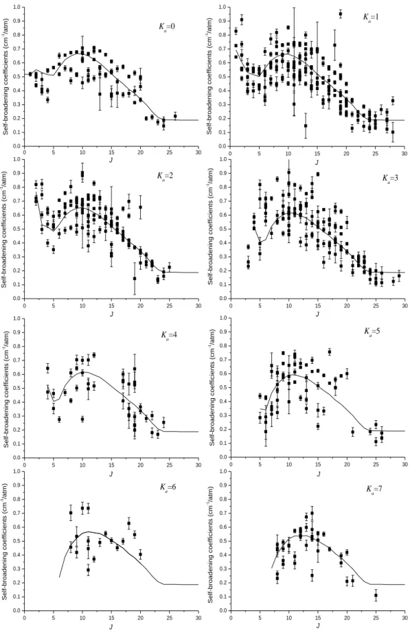
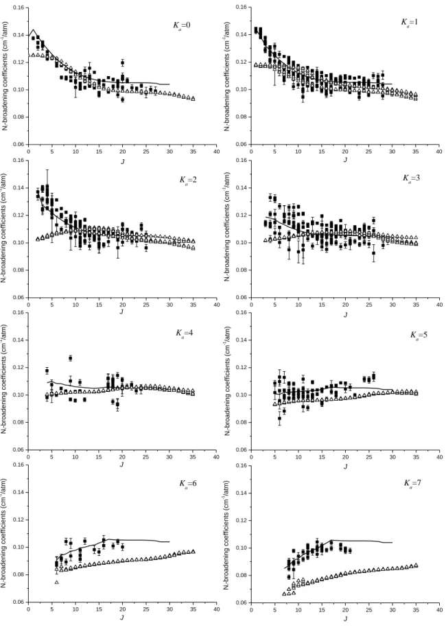
respectively. In Figs. 7 and 8 are plotted, for Ka equal to 0 to 7, both experimental broadening
The 0 J
a parameters represent the J dependence of the broadening parameters for Ka=0,
whereas the a2J parameters describe the influence of the rotational quantum number Ka on
broadening parameters. Despite the important dispersion of the measurements, especially for the self-broadening coefficients, the 0
J
a and 2 J
a parameters are quite smooth and reproduced quite well the rotational dependences in Figs. 3,4,7 and 8. A part of the dispersion of the broadening coefficients in Figs. 1 and 2 is due to the K rotational dependence of the widths modelled by the aJ2 parameters.
3.3. Theoretical calculation for N2-broadening coefficients
3.3.1 The Complex Robert-Bonamy Formalism
The calculations made here are a complex implementation [23-25] of the semi-classical theory of Robert and Bonamy [26]. The complex Robert-Bonamy (CRB) formalism produces the half-width and line shift from a single complex calculation. In this formalism the half-width, , and line shift, , of a ro-vibrational transition fi are given by minus the imaginary part and the real part, respectively, of the diagonal elements of the complex relaxation matrix [27,28]. In computational form and are expressed in terms of the Loiuville scattering matrix
i
n
22 c
v 1 e
RS
2 f ,i,J2,v,b
e
iIS2 f ,i,J2,v,bv,b,J (2)
where n2 is the number density of perturbers and v,b,J
2 represents an average over all trajectories (impact parameter b and initial relative velocity v) and initial rotational state J2 of
the collision partner. S2= RS2+ iIS2 is the second order terms in the successive expansion of
the scattering matrix, which depends on the ro-vibrational states involved and associated collision induced jumps from these levels, on the intermolecular potential and characteristics of the collision dynamics. Note, Eq. (2) generally contains the vibrational dephasing term, S1,
which arises only for transitions where there is a change in the vibrational state. The potential leading to S1 is written in terms of the isotropic induction and London dispersion interactions
which depend on the vibrational dependence of the dipole moment and polarizability of the radiating molecule. These parameters are not available for H2CO and the S1 term has been
component, like H2CO-N2, the effect of the S1 term on the half-width often tends to be small.
The exact form of the S2 term is given in Refs. [23-26].
The intermolecular potential used in the calculations is comprised of an electrostatic component (dipole and quadrupole moments of H2CO with the quadrupole moment of N2 or
with the dipole and quadrupole moments of H2CO) and an atom-atom component. The initial
heteronuclear Lennard-Jones parameters for the atomic pairs are determined using the "combination rules" of Hirschfelder et al. [29]. The atom-atom distance, rij is expressed in
terms of the center of mass separation, R, via the expansion in 1/R of Sack [30] using the formulation of Neshyba and Gamache [31] expanded to 8th order.
The dynamics of the collision process use Robert and Bonamy’s [26] second order in time approximation to the true trajectories, which are based on the isotropic part of the intermolecular potential. These curved trajectories have been shown to accurately model the true trajectories [32].
3.3.2 Parameters for the H2CO-N2 collision system
The wavefunctions used to evaluate the reduced matrix elements are obtained by diagonalizing the Watson Hamiltonian [33] in a symmetric top basis. The wavefunctions for the ground vibrational state of H2CO are determined using the Watson-Hamiltonian constants
of Muller et al. [34] and those for the 2 vibrational state use the Watson constants of Perrin
[35]. The molecular constants for N2 are from Huber and Herzberg [36].
The molecular constants used in the calculations are as follows: The dipole moment is from the work of Fabricant et al. [37], =2.33 D. The quadrupole moments are from Kukolich [38] here reported with H2CO in the IR representation: Qxx=−0.269±0.20 10−26 esu,
Qyy=+0.3295±0.12 10−26 esu, Qzz=−0.0605±0.16 10−26 esu. The quadrupole moment of
nitrogen is from Mulder et al. [39], Qzz=−1.4±0.1 10−26 esu. The starting atom-atom
parameters were obtained using the standard combination rules with the atom-atom parameters for homonuclear diatomics determined by Bouanich [40] by fitting to second virial coefficient data. In the calculations, the atom-atom potential is expanded to eighth-order in the molecular centers of mass separation.
The input Lennard-Jones atom-atom parameters are not as well known as the other parameters; the values can vary by 30% and the values by 5% depending on the source and the values can vary by 69% and the values by 9% depending on whether they were derived using viscosity data or virial data [29]. Depending on how the values were derived it
is possible to find examples in the literature where the parameters for the same interaction pair differ by factors of 2. Thus it appears reasonable to adjust the atom-atom parameters and/or the resulting trajectory parameters provided there are reliable experimental data to fit to. To accomplish this, the measured spectra were studied to identify transitions for which we had high confidence in the measurement. This analysis yielded 39 transitions for the H2CO-N2
system.
For H2CO-N2 there are 6 atom-atom parameters ( HN, HN, CN, CN, ON, and ON)
that need to be adjusted. Starting from the combination rule values, see Table 3, individually each epsilon or sigma value was increased by 5% and calculations made. These results were compared to the values calculated using the combination rule values yielding a sense of how the half-width varies with the atom-atom parameters. Using these changes as a guide the parameters were varied and calculations made and compared with the 39 measured half-widths. After 14 iterations the percent difference went from the initial value of −11.1 to a final value of 0.1. The final atom-atom parameters for the H2CO-N2 system are given in
Table 3. Note, the adjustment of the atom-atom parameters was done without the use of a least-squares technique due to the complexity of the atom-atom potential and the time required for a single calculation (~ 4 hours).
3.3.3 Calculation of half widths at various temperatures
A file of 3713 transitions in the 2, 3, and 5 bands of H2CO [35] in the frequency
range 1620-1840 cm−1 atm−1 was taken and 3296 2 transitions extracted for this study.
Complex Robert-Bonamy calculations of the half-width were made at 7 temperatures (200., 225., 275., 296., 350., 500., and 700. K) by solving Eq. 2. The calculations are for transitions with J=0 to 41 and Ka=0 to 16. The half-widths at 296 K range from roughly 0.02 to 0.128, a
factor of 6.4.
The power law model for the temperature dependence of the half-width was given by Birnbaum [41] by considering a one term intermolecular potential and all on-resonance collisions giving T T0 T0 T n (3)
where n is called the temperature exponent. While modern calculations use hundreds of terms in the intermolecular potential, Eq. (3) remains a reliable model for many systems. However, the correctness of Eq. (3) does need to be tested as discussed below.
The temperature exponent does depend on the temperature range of the fit [42,43]. Here, the temperature exponent was determined for each transition by a least-squares fit of
ln[ (T)/ (T0)] vs. ln[To/T] using five (200K-350K) and seven (200K-700K) temperatures of
the study. The error in the temperature exponent was determined as follows: The temperature exponents were calculated using the half-width values at any two of the temperatures studied. For example, with seven temperatures this yields twenty-one 2-point temperature exponents. The difference between each 2-point temperature exponent and the lease-squares fit value is calculated. The error is taken as the largest of these differences. While this procedure tends to yield the maximum error in the temperature exponent, given the nature of the data and other uncertainties it is thought to be more reasonable than a statistical value taken from the fit.
Discussion
Half-width as a function of the rotational quantum numbers
The half-widths at 296 K are plotted versus an energy ordered index (J(J+1)+Ka-Kc+1) in
Figure 7 where the plot symbols are the Ka values. The roughly vertical columns in the figure
are data with the same J. There appears to be some structure with respect to the Ka with the
largest half-widths belonging to transitions with the smallest Ka values. However, no simple
propensity rule to predict half-widths can be derived from the data.
3.3.4 Temperature dependence of the half-width
The temperature dependence of the N2-broadened half-widths was determined for the
3296 2 band transitions studied in this work using the power law formula, Eq. (3). The
“rule-of-thumb” expression for the temperature exponent given by Birnbaum [41] for a “dipole-quadrupole” system, such as H2CO-N2 states that n=5/6.
Some recent studies have shown that for certain types of radiator-perturber interactions the power law model is questionable. Wagner et al. [44] have observed that for certain transitions of water vapor perturbed by air, N2 or O2 the power law does not correctly
model the temperature dependence of the half-width. This fact was later demonstrated by Toth et al. [45] in a study of air-broadening of water vapor transitions in the region from 696-2163 cm−1. In both studies it was found that the temperature exponent, n, can be negative for many transitions. In such cases the power law model, Eq. (3), is not completely correct. The
mechanism leading to negative temperature exponents is called the resonance overtaking effect and was discussed by Hartmann et al. [46], Wagner et al. [44], and Antony et al. [47]. Thus, in this work the applicability of the power law model was tested.
The values for the temperature dependence of the N2-broadened half-width go from
roughly 0.83 to 0.10. While the range in values is large, there are no negative temperature exponents for this collision system. As stated above the temperature exponents were calculated for 2 temperature ranges; 200-350K, and 200-700K. Figure 8 shows the fits for the 19 15 5 18 15 4 transition for the two temperature ranges. Plotted are ln[ (T)/ (T0)] versus ln[T0/T] where the slope of the fitted line is the value of n. The temperature exponent for the
7 data points is 0.40 (top panel) and that for the 5-point fit is 0.54 (bottom panel). For both cases the correlation coefficient, R, indicates the power law fit is not perfect and the error associated with the 7-point fit is almost 3 times larger than that for the 5-point fit. (Note, the scale of the abscissa is different in each panel.) For atmospheric applications the temperature range of the 5-point fit, 200-350K, is more appropriate and the temperature exponents reported here are those of the 5-point fit. In Fig. 9 ln[ (T)/ (T0)] versus ln[T0/T] is plotted for
the 2 1 1 2 1 2 transition (top panel) and the 20 14 6 19 14 5 transition (lower panel). In
the top panel the fit is quite good (R=0.99995) and the slope, n, is 0.761(0.038). In the lower panels is an example of a high J and Ka transition where n is 0.360(0.240) the fit is not as
good (R=0.9831), which is reflected in the reported error. It is cautioned that there are many transitions for which the power law model does not work well.
In Fig. 10 the temperature exponents for the 3713 N2-broadened transitions of H2CO
are plotted versus the energy ordered index. The dashed line in the plot is the “rule of thumb” value, 5/6. Plots (not shown here) were made with Ka as the plot symbol and different
coordinates for the abscissa but no structure was evident. Figure 10 shows there are large variations in n as a function of the rotational quantum numbers.
3.4. Comparisons
Figure 11 shows the measured half-widths from Refs [48-51] and this work and the calculated half-widths versus J+0.9(Ka/J). The star symbols are the measurements of the 3
band transitions by Cline and Varghese [48], The square symbol is the measurement of Burkart and Schramm on the 4 1 4 5 1 5 transition in the 1 band [49], the open circle with
the plus sign symbol is the measurement of the 3 1 3 3 1 2 transition in the rotation band
[50], the open plus sign symbol is the measurement of the the 3 0 3 3 1 3 transition in the 4
band by Nadler et al. [51], the solid triangles are the measurements of this work. All the measurements have the associated error bars plotted as well. The solid circles are the CRB calculations of the half-widths for 2 transitions. The plot shows the data of refs. [49] and
[51] are low compared with the other measurements. It is not certain if this is an effect of vibrational dependence of the half-widths for these two transitions. The data of Ref. 48 agree somewhat with the measurements made here at low J but the data above J=8 have smaller values than the measurements made here. The calculated half-widths are lower than the measurements made here for low J. For J≥5 the agreement is good. Overall the calculations have a 4.5 % difference when compared to all 258 measurements.
4. Creation of a complete line list
The last edition of HITRAN [13] contain the recent line list of A. Perrin et al. [12] concerning both the 3.6 and 5.7 µm spectral regions (35958 lines), and quite all data for the 0-100 cm−1 spectral region (163 lines). For all these transitions, constant values have been used for both the self- and N2-broadening coefficients, as well as for the temperature dependence of
the N2-broadening coefficients. Table A3 given as supplementary materials is a copy of the
formaldehyde 12H212C16O2 line list from HITRAN 2008 [13], in which self- and N2
broadening coefficients generated with the empirical polynomial expansion together with the parameters of Table 2 (see Section 3.2). The N2-broadening coefficients and its temperature
dependence, calculated using the complex Robert Bonamy formalism for the 2 band (see
Section 3.3), have also been used to complete the HITRAN line list. Then, Table 3 has not really the same format as the one of the HITRAN database since two columns of N2
ACKNOWLEDGEMENTS
REFERENCES
[1] Yokelson RJ, Goode JG, Ward DE, Susott RA, Babbitt RE, Wade DD, Bertschi I, Griffith DWT, Hao WM. Emissions of formaldehyde, acetic acid, methanol, and other trace gases from biomass fires in North Carolina measured by airborne Fourier transform infrared spectroscopy. J of Geophys Res 1999;D104:30109-30125.
[2] Fried A, Sewell S, Henry B, Wert BP, Gilpin T. Tunable diode laser absorption spectrometer for ground-based measurements of formaldehyde. J of Geophys Res 1997;D102:6253-6266.
[3] Fried A, Lee YN, Frost G, Wert B, Henry B, Drummond JR, Hubler G, Jobson T. Airborne CH2O measurements over the North Atlantic during the 1997 NARE campaign:
Instrument comparisons and distributions. J Geophys Res 2002;D107:ACH14-1-21.
[4] Wert BP, Fried A, Rauenbuehler S, Walega J, Henry B. Design and performance of a tunable diode laser absorption spectrometer for airborne formaldehyde measurements. Journal of Geophysical Research 2003;108(D12):ACH1-1-15.
[5] Richter D, Fried A, Wert BP, Walega JG, Tittel FK. Development of a tunable mid-IR difference frequency laser source for highly sensitive airborne trace gas detection Appl Phys B75 2002 281-288
[6] Dahnke H, von Basum G, Kleinermanns K, Hering P, Murts M. Rapid formaldehyde monitoring in ambient air by means of mid-infrared cavity leak-out spectroscopy. Appl Phys 2002;B75:311-316.
[7] Coheur PF, Herbin H, Clerbaux C, Hurtmans D, Wespes C, Carleer M, Turquety S, Rinsland CP, Remedios J, Hauglustaine D, Boone CD, Bernath PF. ACE-FTS observation of a young biomass burning plume: first reported measurements of C2H4, C3H6O, H2CO and
PAN by infrared occultation from space. Atmos Chem Phys 2007;7:5437-5446.
[8] Wagner V, Schiller C, Fischer H. Formaldehyde measurements in the marine boundary layer of the Indian Ocean during the 1999 INDOEX cruise of the R/V Ronald H. Brown. J Geophys Res 2001;D106:28528-28538.
[9] Steck T, Glatthor N, von Clarmann T, Fischer H, Flaud JM, Funke B, Grabowski U, Höpfner M, Kellmann S, Linden A, Perrin A, Stiller GP. Retrieval of global upper tropospheric and stratospheric formaldehyde (H2CO) distributions from high-resolution
MIPAS-Envisat spectra. Atmos Chem Phys 2008;8:463-470.
[10] Herndon SC, Zahniser MS, Nelson DD Jnr, Shorter J, McManus JB, Jimenez R, Warneke C, de Gouw JA. Airborne measurements of HCHO and HCOOH during the New England Air Quality Study 2004 using a pulsed quantum cascade laser spectrometer. J of Geophys Res 2007;112(D10): D10S03-1-15.
[11] Rinsland CP, Goldman A. Infrared spectroscopic measurements of tropospheric trace gases. Appl Opt 1992; 31:6969-6971.
[12] A. Perrin, D. Jacquemart, F. Kwabia Tchana, and N. Lacome. Absolute line intensities and new linelists for the 5.7 and 3.6 µm bands of formaldehyde. JQSRT 2009;110:700-16. [13] Rothman LS, Gordon IE, Barbe A, Chris Benner D, Bernath PF, Birk M, Brown LR, Boudon V, Champion J-P, Chance K, Coudert LH, Dana V, Fally S, Flaud J-M, Gamache RR, Goldman A, Jacquemart D, Lacome N, Mandin J-Y, Massie ST, Mikhailenko S, Orphal J, Perevalov V, Perrin A, Rinsland CP, Šimečková M, Smith MAH, Tashkun
S, Tennyson J, Toth RA, Vandaele AC, Vander Auwera J. The HITRAN 2008 Molecular Spectroscopic Database. J. Quant. Spectrosc. Radiat. Transfer 110,533-572 (2009).
[14] Jacquemart D, Mandin JY, Dana V, Picqué N, Guelachvili G. A multispectrum fitting procedure to deduce molecular line parameters. Application to the 3-0 band of 12C16O. Eur Phys J D 2001;14:55-69.
[15] Nemtchinov V, Sung, K, Varanasi P. Measurements of line intensities and half-widths in the 10-μm bands of 14NH3. JQSRT 2004;83:243-65.
[16] Predoi-Cross A, Hambrook K, Brawley-Tremblay S, Bouanich JP, Malathy Devi V, Smith MAH. Room-temperature broadening and pressure-shift coefficients in the ν2 band of
CH3D–O2: Measurements and semi-classical calculations. J Mol Spectrosc 2006;236;75-90.
[17] Predoi-Cross A, Hambrook K, Brawley-Tremblay S, Bouanich JP, Malathy Devi V, Smith MAH. Measurements and theoretical calculations of N2-broadening and N2-shifting
coefficients in the ν2 band of CH3D. J Mol Spectrosc 2006;235;35-53.
[18] Lepère M, Blanquet G, Walrand J, Bouanich JP. K-dependence of broadening coefficients for CH3F-N2 and for other systems involving a symmetric top molecule. J Mol
Spectrosc 2000;517-518:493-502.
[19] Chackerian C, Brown LR, Lacome N, Tarrago G. Methyl Chloride ν5 Region Lineshape
Parameters and Rotational Constants for the ν2, ν5, and 2ν3 Vibrational Bands. J Mol
Spectrosc 1998;191:148-57.
[20] Bouanich JP, Blanquet G, Walrand J. Theoretical O2- and N2-Broadening Coefficients of
CH3Cl Spectral Lines. J Mol Spectrosc 1993;161:416-26.
[21] Levy A, Lacome N, Tarrago G. Hydrogen- and Helium-Broadening Phosphine Lines. J Mol Spectrosc 1993;157:172-81.
[22] Jacquemart D, Kwabia Tchana F, Lacome N, Kleiner I. A complete set of line parameters for CH3Br in the 10-µm spectral region. JQSRT 2007;105:264-302.
[23] Lynch R. Half-widths and line shifts of water vapor perturbed by both nitrogen and oxygen. Ph.D. dissertation, University of Massachusetts Lowell, June, 1995.
[24] Lynch R, Gamache RR, Neshyba SP. Fully Complex Implementation of the Robert-Bonamy Formalism: Halfwidths and Line Shifts of H2O Broadened by N2, J. Chem. Phys.
1996; 105: 5711-21.
[25] amache RR, Lynch R, Neshyba SP. New Developments in the Theory of Pressure-Broadening and Pressure-Shifting of Spectral Lines of H2O: The Complex Robert-Bonamy
Formalism, J. Quant. Spectrosc. Radiat. Transfer 1998; 59: 319-35
[26] Robert D, Bonamy J. Short range force effects in semiclassical molecular line broadening calculations, Journal De Physique 1979; 20: 923-43.
[27] Baranger M. General impact theory of pressure broadening, Phys Rev 1958; 112: 855-65.
[28] Ben-Reuven A, Spectral Line Shapes in Gases in the Binary-Collision Approximation, Adv. Chem. Phys., Prigogine I and Rice SA, Editors. 1975, Academic Press: New York. p. 235.
[29] Hirschfelder JO, Curtiss CF, Bird RB. Molecular Theory of Gases and Liquids, Wiley, New York 1964.
[30] Sack RA. Two-Center Expansion for the Powers of the Distance Between Two Points, J. Math. Phys. 1964; 5: 260-8.
[31] Neshyba SP, Gamache RR. Improved Line Broadening Coefficients for Asymmetric Rotor Molecules: Application to Ozone Perturbed by Nitrogen., J. Quant. Spectrosc. Radiat. Transfer 1993; 50: 443-53.
[32] Neshyba SP, Lynch R, Gamache RR, Gabard T, Champion J-P. Pressure Induced Widths and Shifts for the ν3 band of Methane, J. Chem. Phys. 1994; 101: 9412-21.
[33] Watson JKG. Determination of centrifugal Distortion Coefficients of Asymmetric- Top Molecules, J. Chem. Phys. 1967; 46: 1935-49.
[34] Muller HSP, Winnewisser G, Demasion J, Perrin A, Valentin A. The Ground State Spectroscopic Constants of Formaldehyde, J. Mol. Spectrosc. 2000; 200: 143-4.
[35] Perrin A. Watson Hamiltonian constants for the ν2 band of H2CO and H2CO linelist,
private communication, Laboratoire Inter-Universitaire des Systemes Atmospheriques (LISA), CNRS, Universite Paris XII, Paris, France, 2007.
[36] Huber KP, Herzberg G. Molecular Spectra and Molecular Structure: Constants of Diatomic Molecules, Van Nostrand, New York 1979.
[37] Fabricant B, Krieger D, Muebnter JS. Molecular beam electric resonance study of formaldehyde, thioformaldehyde, and ketene, J. Chem. Phys. 1977; 67: 1576-86.
[38] Kukolich SG. Molecular Beam Measurements of the Magnetic Susceptibility Anisotrophies and Molecular Quadrupole Moment in H2CO, J. Chem. Phys. 1971; 54: 8-11.
[39] Mulder F, van Dijk G, van der Avoird A. Multipole moments, polarizabilities and anisotropic long range interaction coefficients for N2, Mol. Phys. 1980; 39: 407-25.
[40] Bouanich J-P. Site-Site Lennard- Jones Potential Parameters for N2 ,O2 , H2, CO and
CO2, J. Quant Spectrosc. Radiat. Transfer 1992; 47: 243-50.
[41] Birnbaum G. Microwave Pressure Broadening and its Application to Intermolecular Forces, Advances in Chem. Phys. 1967; 12: 487-548.
[42] L. R. Brown,C. M. Humphrey and R. R. Gamache, “CO2-broadened water in the pure
rotation and 2 fundamental regions,” J. Mol. Spectrosc. 246, 1-21, 2007.
[43] R. R. Gamache and A. L. Laraia, “N2-, O2-, and air-broadened half-widths, their
temperature dependence, and line shifts for the rotation band of H216O,” in press J. Mol.
Spectrosc., 2009.
[44] Wagner G, Birk M, Gamache RR, Hartmann J-M. Collisional parameters of H2O lines:
effects of temperature, J. Quant. Spectrosc. Radiat. Transfer 2005; 92: 211-30.
[45] Toth RA, Brown LR, Smith MAH, Malathy Devi V, Chris Benner D, Dulick M. Air-broadening of H2O as a function of temperature: 696-2163 cm-1, J. Quant. Spectrosc. Radiat.
Transfer 2006; 101: 339-66.
[46] Hartmann JM, Taine J, Bonamy J, Labani B, Robert D. Collisional broadening of rotation-vibration lines for asymmetric-top molecules II. H2O diode laser measurements in the
400-900 K range; calculations in the 300-2000 K range, J. Chem. Phys. 1987; 86: 144-56. [47] Antony BK, Neshyba S, Gamache RR. Self-broadening of water vapor transitions via the complex Robert-Bonamy theory, J. Quant. Spectrosc. Radiat. Transfer 2006; 105: 148-63.
[48] Cline DS, Varghese PL. High resolution spectral measurements in the ν3 band of
formaldehyde using a tunable IR diode laser, Applied Optics 1988; 27: 3219-24.
[49] Burkart M, Schramm B. Foreign gasbroadening of an IR absorption line of formaldehyde, J. Mol. Spectrosc. 2003; 217: 153-6.
[50] Srivastava GP, Gautam HO, Kumar A. Microwave pressure broadening studies of some molecules, J. Phys. B: Atom. Molec. Phys. 1973; 6: 743-55.
[51] Nadler S, Daunt SJ, Reuter DC. Tunable diode laser measurements of formaldehyde foreign gas broadening parameters and line strengths in the 9-11 μm region, Appl. Opt. 1987;
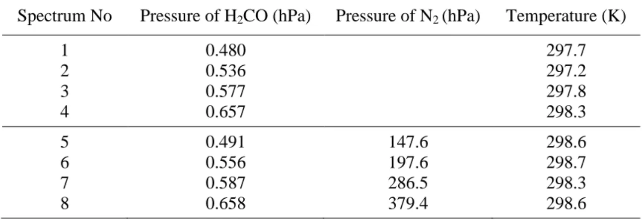
Table 1. Absorbing sample Natural H2CO (98.624 % of H2C16O) Estimated purity ~98.9 % Experimental conditions SNR 75-100 Absorption path 30 cm
Spectrum No Pressure of H2CO (hPa) Pressure of N2 (hPa) Temperature (K)
1 0.480 297.7 2 0.536 297.2 3 0.577 297.8 4 0.657 298.3 5 0.491 147.6 298.6 6 0.556 197.6 298.7 7 0.587 286.5 298.3 8 0.658 379.4 298.6
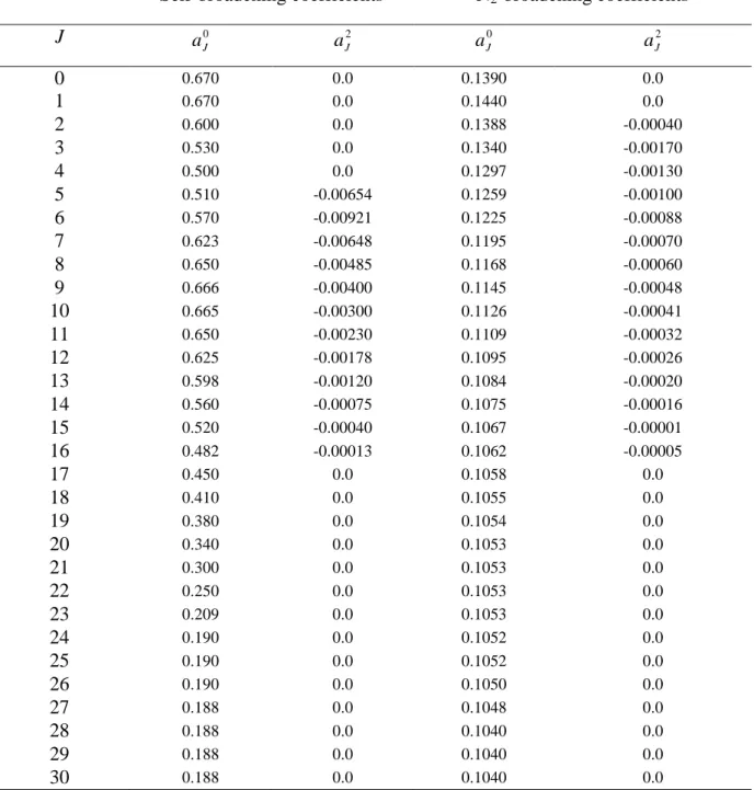
Table 2. Parameters 0 J
a and 2 J
a retained for the calculation of the self- and N2-broadening
coefficients using Eq. (1).
Self-broadening coefficients N2-broadening coefficients
J 0 J a aJ2 aJ0 aJ2 0 0.670 0.0 0.1390 0.0 1 0.670 0.0 0.1440 0.0 2 0.600 0.0 0.1388 -0.00040 3 0.530 0.0 0.1340 -0.00170 4 0.500 0.0 0.1297 -0.00130 5 0.510 -0.00654 0.1259 -0.00100 6 0.570 -0.00921 0.1225 -0.00088 7 0.623 -0.00648 0.1195 -0.00070 8 0.650 -0.00485 0.1168 -0.00060 9 0.666 -0.00400 0.1145 -0.00048 10 0.665 -0.00300 0.1126 -0.00041 11 0.650 -0.00230 0.1109 -0.00032 12 0.625 -0.00178 0.1095 -0.00026 13 0.598 -0.00120 0.1084 -0.00020 14 0.560 -0.00075 0.1075 -0.00016 15 0.520 -0.00040 0.1067 -0.00001 16 0.482 -0.00013 0.1062 -0.00005 17 0.450 0.0 0.1058 0.0 18 0.410 0.0 0.1055 0.0 19 0.380 0.0 0.1054 0.0 20 0.340 0.0 0.1053 0.0 21 0.300 0.0 0.1053 0.0 22 0.250 0.0 0.1053 0.0 23 0.209 0.0 0.1053 0.0 24 0.190 0.0 0.1052 0.0 25 0.190 0.0 0.1052 0.0 26 0.190 0.0 0.1050 0.0 27 0.188 0.0 0.1048 0.0 28 0.188 0.0 0.1040 0.0 29 0.188 0.0 0.1040 0.0 30 0.188 0.0 0.1040 0.0
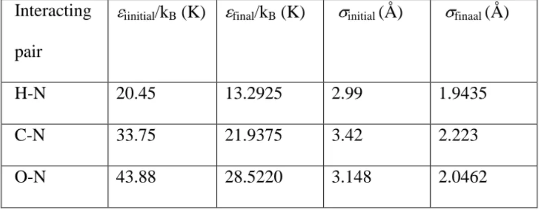
Table 3. Initial and final atom-atom parameters for the H2CO-N2 collision systems
Interacting
pair
iinitial/kB (K) final/kB (K) initial (Å) finaal (Å)
H-N 20.45 13.2925 2.99 1.9435
C-N 33.75 21.9375 3.42 2.223
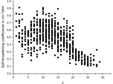
Fig 1: Self-broadening coefficients versus J. 0 5 10 15 20 25 30 0,0 0,1 0,2 0,3 0,4 0,5 0,6 0,7 0,8 0,9 1,0 Sel f-b ro a d e n in g co e ff ici e n ts in cm -1 /a tm J
Fig 2: N2-broadening coefficients versus J.
0 5 10 15 20 25 30 0,00 0,02 0,04 0,06 0,08 0,10 0,12 0,14 0,16 N2 -b ro a d e n in g co e ff ici e n ts in cm -1 /a tm J
Fig.3: Rotational dependence with respect to Ka2 for self-broadening coefficients with J=8. 0 10 20 30 40 50 0,0 0,1 0,2 0,3 0,4 0,5 0,6 0,7 0,8 0,9 1,0 Sel f-b ro a d e n in g co e ff ici e n ts in cm -1 /a tm Ka2
Fig.4: Rotational dependence with respect to Ka2 for N2-broadening coefficients with J=8.
0 10 20 30 40 50 0,00 0,03 0,06 0,09 0,12 0,15 N2 -b ro a d e n in g co e ff ici e n ts in cm -1 /a tm K a 2
Fig.5: Parameters 0 J
a and 2 J
a deduced from the fit of the measured self-broadening coefficients using Eq. (1). The error bars are 1SD. The continuous line symbolizes a manual smooth of these parameters.
0 5 10 15 20 25 30 0.00 0.05 0.10 0.15 0.20 J aJ 2 p a ra m e te rs 0 5 10 15 20 25 30 0.1 0.2 0.3 0.4 0.5 0.6 0.7 0.8 J aJ 0 p a ra m e te rs
Fig.6: Parameters 0 J
a and 2 J
a deduced from the fit of the measured N2-broadening coefficients
using Eq. (1). The error bars are 1SD. The continuous line symbolizes a manual fit of these parameters. 0 5 10 15 20 25 30 0.06 0.08 0.10 0.12 0.14 0.16 aJ 0 param eters J 0 5 10 15 20 25 30 -0.015 -0.010 -0.005 0.000 0.005 J aJ 2 p a ra m e te rs
Fig. 7: Self-broadening coefficients measurements are plotted for each value of Ka values
from 0 up to 7. The error bars are 1SD. The continuous line represents calculation based on an empirical expansion (see Eq. (1)) and parameters of Table 2. Open triangles are the theoretical calculation using the Complex Robert-Bonamy Formalism for ∆Ka = 0 transitions
(see Section 3.3). 0 5 10 15 20 25 30 0.0 0.1 0.2 0.3 0.4 0.5 0.6 0.7 0.8 0.9 1.0 K a=1 Sel f-b ro a d e n in g co e ff ici e n ts (cm -1/a tm ) J 0 5 10 15 20 25 30 0.0 0.1 0.2 0.3 0.4 0.5 0.6 0.7 0.8 0.9 1.0 K a=0 J Sel f-b ro a d e n in g co e ff ici e n ts (cm -1/a tm ) 0 5 10 15 20 25 30 0.0 0.1 0.2 0.3 0.4 0.5 0.6 0.7 0.8 0.9 1.0 J Se lf -b ro a d e n in g co e ff ici e n ts (cm -1/a tm ) K a=2 0 5 10 15 20 25 30 0.0 0.1 0.2 0.3 0.4 0.5 0.6 0.7 0.8 0.9 1.0 J Sel f-b ro a d e n in g co e ff ici e n ts (cm -1/a tm ) Ka=3 0 5 10 15 20 25 30 0.0 0.1 0.2 0.3 0.4 0.5 0.6 0.7 0.8 0.9 1.0 J Ka=4 Se lf -b ro a d e n in g co e ff ici e n ts (cm -1/a tm ) 0 5 10 15 20 25 30 0.0 0.1 0.2 0.3 0.4 0.5 0.6 0.7 0.8 0.9 1.0 K a=5 J Sel f-b ro a d e n in g co e ff ici e n ts (cm -1/a tm ) 0 5 10 15 20 25 30 0.0 0.1 0.2 0.3 0.4 0.5 0.6 0.7 0.8 0.9 1.0 J Sel f-b ro a d e n in g co e ff ici e n ts (cm -1/a tm ) Ka=6 0 5 10 15 20 25 30 0.0 0.1 0.2 0.3 0.4 0.5 0.6 0.7 0.8 0.9 1.0 K a=7 J Se lf -b ro a d e n in g co e ff ici e n ts (cm -1/a tm )
Fig. 8: N2-broadening coefficients measurements are plotted for each value of Ka values from
0 up to 7. The error bars are 1SD. The continuous line represents calculation based on an empirical expansion (see Eq. (1)) and parameters of Table 2. Open triangles are the theoretical calculation using the Complex Robert-Bonamy Formalism for ∆Ka = 0 transitions
(see Section 3.3). 0 5 10 15 20 25 30 35 40 0.06 0.08 0.10 0.12 0.14 0.16 Ka=0 N2 -b ro a d e n in g co e ff ici e n ts (cm -1/a tm ) J 0 5 10 15 20 25 30 35 40 0.06 0.08 0.10 0.12 0.14 0.16 J N 2 -b ro a d e n in g co e ff ici e n ts (cm -1 /a tm ) Ka=1 0 5 10 15 20 25 30 35 40 0.06 0.08 0.10 0.12 0.14 0.16 K a=2 J N2 -b ro a d e n in g co e ff ici e n ts (cm -1/a tm ) 0 5 10 15 20 25 30 35 40 0.06 0.08 0.10 0.12 0.14 0.16 J N2 -b ro a d e n in g co e ff ici e n ts (cm -1/a tm ) Ka=3 0 5 10 15 20 25 30 35 40 0.06 0.08 0.10 0.12 0.14 0.16 Ka=4 J N2 -b ro a d e n in g co e ff ici e n ts (cm -1/a tm ) 0 5 10 15 20 25 30 35 40 0.06 0.08 0.10 0.12 0.14 0.16 Ka=5 J N 2 -b ro a d e n in g co e ff ici e n ts (cm -1 /a tm ) 0 5 10 15 20 25 30 35 40 0.06 0.08 0.10 0.12 0.14 0.16 J N2 -b ro a d e n in g co e ff ici e n ts (cm -1/a tm ) Ka=6 0 5 10 15 20 25 30 35 40 0.06 0.08 0.10 0.12 0.14 0.16 Ka=7 J N 2 -b ro a d e n in g co e ff ici e n ts (cm -1 /a tm )