HAL Id: hal-03017880
https://hal.archives-ouvertes.fr/hal-03017880
Submitted on 4 Jan 2021HAL is a multi-disciplinary open access archive for the deposit and dissemination of sci-entific research documents, whether they are pub-lished or not. The documents may come from teaching and research institutions in France or abroad, or from public or private research centers.
L’archive ouverte pluridisciplinaire HAL, est destinée au dépôt et à la diffusion de documents scientifiques de niveau recherche, publiés ou non, émanant des établissements d’enseignement et de recherche français ou étrangers, des laboratoires publics ou privés.
Impact of the hydrological regime and forestry
operations on the fluxes of suspended sediment and
bedload of a small middle-mountain catchment
S. Cotel, D. Viville, S. Benarioumlil, P. Ackerer, M.C. Pierret
To cite this version:
S. Cotel, D. Viville, S. Benarioumlil, P. Ackerer, M.C. Pierret. Impact of the hydrological regime and forestry operations on the fluxes of suspended sediment and bedload of a small middle-mountain catchment. Science of the Total Environment, Elsevier, 2020, 743, pp.140228. �10.1016/j.scitotenv.2020.140228�. �hal-03017880�
Journal Pre-proof
Impact of the hydrological regime and forestry operations on the
fluxes of suspended sediment and bedload of a small
middle-mountain catchment
S. Cotel, D. Viville, S. Benarioumlil, P. Ackerer, M.C. Pierret
PII:
S0048-9697(20)33749-9
DOI:
https://doi.org/10.1016/j.scitotenv.2020.140228
Reference:
STOTEN 140228
To appear in:
Science of the Total Environment
Received date:
8 February 2020
Revised date:
29 May 2020
Accepted date:
13 June 2020
Please cite this article as: S. Cotel, D. Viville, S. Benarioumlil, et al., Impact of the
hydrological regime and forestry operations on the fluxes of suspended sediment and
bedload of a small middle-mountain catchment, Science of the Total Environment (2020),
https://doi.org/10.1016/j.scitotenv.2020.140228
This is a PDF file of an article that has undergone enhancements after acceptance, such
as the addition of a cover page and metadata, and formatting for readability, but it is
not yet the definitive version of record. This version will undergo additional copyediting,
typesetting and review before it is published in its final form, but we are providing this
version to give early visibility of the article. Please note that, during the production
process, errors may be discovered which could affect the content, and all legal disclaimers
that apply to the journal pertain.
Journal Pre-proof
Impact of the hydrological regime and forestry operations on the fluxes of suspended
sediment and bedload of a small middle-mountain catchment
S. Cotel1*, D. Viville1, S. Benarioumlil1, P. Ackerer1, M.C. Pierret 1
1
Laboratoire d’Hydrologie et de Géochimie de Strasbourg (LHyGeS), UMR 7517, Université de Strasbourg - Centre National de la Recherche Scientifique (CNRS) - École Nationale du Génie de l'Eau et de l'Environnement de Strasbourg (ENGEES), 1 rue Blessig, 67084
Strasbourg, France
E-mail addresses: *[email protected] (S. Cotel) / [email protected] (D. Viville) / [email protected] (S. Benarioumlil) / [email protected] (P. Ackerer) / [email protected] (M.C. Pierret)
Journal Pre-proof
1. Introduction
Mechanical erosive processes play a key role in the global landscape structure and the evolution of terrestrial continental surfaces (Tucker, 2015). They generate sediments (bedload and suspended matter), which will be mainly transported by rivers with potential sedimentation, storage, or remobilization phases. The characteristics of the solid transport may impact our environment and human activities (agricultural soil losses, silting of lakes, estuaries, dams or harbors, and clogging of river beds). In addition, the suspended sediments (SS) are an important vector for many elements, including pollutants (pesticides, heavy metals, and radionuclides; Cánovas et al., 2012; He et al., 2015; Iwagami et al., 2016) and nutrients (Martínez-Carreras et al., 2012). At the watershed scale, the annual export flux of SS generally represents more than two-thirds of the annual solid flux (Serrat, 1999; Mathys, 2006; Lenzi et al., 2003; Vericat and Batalla, 2006; Pratt-Sitaula et al., 2007) and more than the annual dissolved flux adjusted for atmospheric inputs (Serrat, 1999; Millot et al., 2002; Viville et al., 2012). The accurate quantification of SS fluxes and the knowledge of their intra- and inter-annual dynamics at the watershed scale are, therefore, essential for understanding the biogeochemical functioning of ecosystems.
The natural SS flux of a river can be explained by several parameters related to the characteristics of the watershed (area, slope, geology, soil type, and land cover; Mueller and Pitlick, 2013; Bywater-Reyes et al., 2017) and climatic conditions (rainfall, snow, temperature, and solar radiation; Syvitski and Milliman, 2007). The SS concentration typically shows considerable temporal variability, and a large portion of the annual SS flux is often carried during some major thunderstorm events (Coynel et al., 2004; Moatar et al., 2006; Mano et al., 2009; Duvert et al., 2011). Furthermore, natural SS flux in rivers can be disturbed by anthropogenic activities (Tarolli and Sofia, 2016), including urbanization, mining, agriculture (Glendell and Brazier, 2014), forestry (Gomi et al., 2005), and, more generally, land use planning (Mueller et al., 2009). Among them, forest management can affect and significantly increase SS concentrations due to tree cutting but also to the building of forest roads, skid trails, and stream crossings (Grant and Wolff, 1991; Karwan et al., 2007; Bywater-Reyes et al., 2017; Cristan et al., 2016). For example, Motha et al. (2003) found that the harvested areas contribute 1.2 to 5 times more to SS flux than undisturbed forest plots, and unsealed forest roads generate 20 to 60 times more SS export than undisturbed forests. Even if forest road and skid trail areas often constitute less than 10% of the catchment area, their contribution to SS flux is not negligible (Grayson et al., 1993; Cornish, 2001; Jordan, 2006). Indeed, deforestation reduces vegetal transpiration and precipitation interception with the loss of foliage, and it enhances snowfall and
Journal Pre-proof
thawing rates with the change in aerodynamic and meteorological conditions in cut areas (Macdonald et al., 2003; Schelker et al., 2013). These elements contribute to an increase in surface runoff, peak discharges, annual stream discharge, and thus in the sediment carrying capability of the hydrosystem (Martin et al., 2000; Hotta et al., 2007). Furthermore, mechanized tree harvesting increases the natural proportion of bare and unconsolidated soil, which increases the proportion of easily exported materials by surface runoff during rain or snowmelt events. Forest roads and skid trails create more compact and less permeable surfaces with less tortuous paths for flow, increasing surface runoff and thus erosion and sediment transport during rainy periods. When the silvicultural access network is hydraulically connected with brooks by stream crossings, it has a disproportionally higher potential to introduce sediments into those brooks (Taylor et al., 1999; Cornish, 2001; Aust et al., 2011; Brown et al., 2013; Lang et al., 2018).
In contrast to large regional catchments, the undisturbed SS flux of small watersheds (< 10 km2) has been studied to a lesser extent (Vanmaercke et al., 2011; Merchán et al., 2019) and its dynamics are still poorly understood (Vansickle and Beschta, 1983). Furthermore, the hydrology of some small watersheds is complex with bimodal hydrographs. They are the catchment’s response to significant precipitation where the first peak coincides to the rain event, and the second peak is broader and lagged in time (Martinez-Carreras et al., 2016). To our knowledge, few studies address the impact of this type of hydrological functioning on the dynamics of the solid export flux. Besides, these studies were conducted on a limited number of storm or snowmelt events (Heathwaite et al., 1989; Hattanji and Onda, 2004; Langlois et al., 2005). Furthermore, the impact of forestry operations on the dynamics of SS production and export is often estimated with a low sampling frequency (weekly or less; Grayson et al., 1993; Cornish, 2001; Nisbet et al., 2002; Webb et al., 2012; Guevara et al., 2015; Witt et al., 2016; Hancock et al., 2017) and/or with samples taken only during some (not necessarily the most relevant) high-flow events (Grayson et al., 1993; Cornish, 2001; Motha et al., 2003; Hotta et al., 2007; Webb et al., 2012; Witt et al., 2016; Hancock et al., 2017). This may reduce the accuracy of the annual SS flux estimation and thus limit the scope of the studies.
In this context, the main objectives of this work are to estimate the impact of i) the hydrological regime and ii) forestry operations on the solid exports of a headwater catchment, based on an accurate monitoring of SS concentration and exported bedload quantity over several years. The watershed is located in a temperate middle-mountain region with managed forests for several centuries. The hydrological functioning of this catchment includes frequent single-peak hydrographs and some double-peak hydrographs mainly occurring during the
Journal Pre-proof
snowmelt periods (Viville and Gaumel, 2004). Furthermore, during the studied period, in 2012 and 2014, two phases of partial forest harvesting occurred in the lower part of the catchment. The small-scale forestry operations consisted of mechanized clear-cutting on steep plots and required the setup of skid trails and stream crossings.
In detail, this study will seek to highlight the major role of delayed-flow events including snowmelt in the solid export dynamics at the outlet of the catchment and to identify and characterize the potential impacts of the forestry operations on those exports. The first step was to develop a protocol to accurately estimate SS concentrations and fluxes at the hydrological event and year scale.
2. Materials and methods
2.1. Site description
The Strengbach catchment is the study site of the Observatoire Hydro-Géochimique de l'Environnement (OHGE; http://ohge.unistra.fr/). It was selected in 1986 to study and understand the impact of acid rain on the forested ecosystem (Probst et al., 1990; Pierret et al., 2019). Then, it was progressively and extensively used to understand the main hydrobiogeochemical processes occurring in this type of ecosystem, using a large diversity of geochemical tracing and geochronological approaches (Pierret et al., 2014; Schmitt et al., 2017 and 2018; Prunier et al., 2015; Chabaux et al., 2017 and 2019) and, more recently, hydrogeochemical modeling (Beaulieu et al., 2016; Weill et al., 2017; Maquin et al., 2017; Belfort et al., 2018; Ackerer et al., 2018; Weill et al., 2019). Labeled in 2007 by the Institut National des Sciences de l’Univers (INSU) of the Centre National de la Recherche Scientifique (CNRS) as a national observatory, the Strengbach catchment is currently one of the reference observatories of the French network of critical zone observatories (OZCAR; http://www.ozcar-ri.org). For almost 35 years, meteorological and hydrological data have been monitored continuously (for recent reviews on the catchment, see Viville et al., 2017; Pierret et al., 2018).
The Strengbach catchment is a small watershed (0.8 km²) located on the eastern side of the Vosges massif (France) at elevations between 883 m and 1,146 m with rather important slopes (mean slope is 15°). Between 1987 and 2016, the mean annual temperature was 6 °C (mean monthly temperature ranged from -2 °C to 14 °C), and the mean annual precipitation was 1,385 mm, with in average 19% snow. The mean annual runoff was
Journal Pre-proof
809 mm, corresponding to a mean discharge of 21 L.s-1. The main stream is perennial, with high water fluxes during the snowmelt period and low water fluxes during the summer season. A variable saturated area (between 0.25% and 3% of the catchment area) is located in the valley bottom close to the outlet and connected to the stream. This saturated area plays an essential hydrological and geochemical role (Idir et al., 1999; Ladouche et al., 2001; Pierret et al., 2014; see Sect. 3.1.1).
The catchment bedrock is Brézouard granite, a Ca- and Mg-poor granite formed 3322 Ma ago (Boutin et al., 1995). This granite was fractured and hydrothermally altered with a stronger degree of hydrothermal overprinting in the northern part than in the southern part of the catchment (Fichter et al., 1998; Pierret et al., 2014). The soils, of the acid brown to ochreous podzolic series, have an average depth of 1 m.
The whole catchment is a commercially managed forest, and the plantation ages range between 50 and 170 years. Before spring 2012, the forest covered 83% of the catchment and was composed of 80% spruces (Piceas abies) and 20% beeches (Fagus sylvatica). Forest roads (2%) and natural openings (15%) occupied the remaining 17%. The majority of these natural openings, formerly wooded, is due to windfall and sometimes tree cuts following insect epidemics. Another type of natural opening exists in the bottom of the catchment in the frequently saturated area where no woody species can grow, and the soil is covered with small plants adapted to wetlands such as sphagnum mosses, rush (Juncus effuses), and herb (Scirpus sylvaticus).
The open-field precipitation was measured in a clearing at the top of the catchment (Fig. 1) using a tipping bucket gauge connected to a data logger (Campbell model CR10x) at a 10-minute time step. The open-field precipitation at the catchment scale was obtained by the spatialization of local measurements as detailed in previous studies (Pierret et al., 2019). At the catchment outlet, an H-flume hydraulically linked to a stilling well equipped with an immersed ultrasonic probe connected to a data logger (Alcyr model Cyr2) enabled a high-frequency record of the stream water stage. The acquisition high-frequency of the water stage data was 30 measurements per hour. The discharge was computed using an established stage-discharge relationship.
The SS and the bedload fluxes were evaluated according to various methodologies (different methods and frequencies).
2.2. Outlet SS flux estimation
Journal Pre-proof
The SS fluxes were mainly estimated for 4 years since 2013 based on high-frequency sampling. However, a former methodology allowed an estimation of the SS fluxes since 2005 based on fortnightly manual sampling (Viville et al., 2012). Notice that the year, for example 2013, refers to the sampling year beginning on December 8, 2012 (the starting day of the high-frequency SS flux study) and ending on December 8, 2013.
2.2.1. Field sampling and measurements
Beginning January 2004, 2 L water were sampled manually every two weeks at the catchment outlet (see Fig. 1) to measure the SS concentration. Collected in a stream section with well-mixed waters, these manual samples are considered representative of the brook water.
Beginning December 8, 2012, two automatic water samplers (Isco models 3700 and 2900) were installed for both regular and flood events sampling to improve the SS flux estimation. The high-flow sampler was managed by the Alcyr data logger and activated by a predetermined threshold overrun-causing taking of samples on the rising and falling limbs of the hydrograph. The chosen time step for the high-flow sampler ranged from one sample per 10 min for thunderstorm events to one sample per 4 or 8 hr for long-lasting events. The regular sampler had a sampling frequency of 16 hr in accordance with a fortnight sampling capacity. The volumes of the samples were 1 L and 0.5 L for regular and high-flow samplers, respectively, related to the higher SS concentrations expected during flood events.
SS measurements have to address some specific characteristics for small middle-mountain catchments such as frequent low-water levels and long periods of frost in winter. For those catchments, accurate monitoring of the SS flux with automatic water sampling requires i) the minimization of the analytical uncertainty by means of a suitable laboratory method, ii) a good representativeness of the automatic samples in all hydrological conditions, and iii) the protection of the water sampling systems from cold winter temperatures. An evaluation of the selected sampling method following these three items is given in the supplementary information A.1, A.2, and A.3. In the last months of the first study year, the sampling method was improved. The main problems of the initial sampling configuration were the overestimation of the stream SS concentration using automatic samples, especially during low-water periods, and the significant number of missing samples during the cold season. The changes in the sampling configuration (use of new sampling strainers and attachment system, reduction of the stream bed width, and heating of the sampling pipes) led to a significant improvement in the representativeness
Journal Pre-proof
of the water samples collected by the automatic samplers and decrease in the number of missing samples. Indeed, for discharges of less than 9 L.s-1, the weighted least-squared errors between the measured concentrations by automatic sampling and the measured concentrations by manual sampling were 14.6 for the first year and 0.07 for the following 3 years. Similarly, the number of missing 16-hr samples during the cold season (December 1-March 31) decreased from 41 (the first year) to an average of 2 (the following 3 years) although the numbers of frost days were quite the same for each year.
2.2.2. SS concentration measurement protocol
Water samples were filtered through a nitrocellulose membrane (Millipore) with a 0.45 μm pore diameter. Each filter was previously dried in an oven at 60 °C during 24 hr and then weighed on a precision scale. After filtration, the filter was similarly dried and weighed. The SS concentration was calculated according to the following formula:
where C(t) (g.L-1) is the SS concentration in the water sample at sampling time t, mF and mN (g) are the dry filter
mass after and before filtration, respectively, and V(t) (L) is the collected water sample volume.
The uncertainty in SS concentration was estimated experimentally and includes the analytical error and the sampling error linked to the SS concentration variability in all stream cross-sections. This variability is, of course, unknown when a single water sample is carried out per section. This uncertainty was evaluated under high-flow and low-water conditions using two different strategies, which are detailed in supplementary information A.4. The global experimental uncertainty was 8.0% and 11.2% for, respectively, high-flow and low-water conditions.
2.2.3. Data quality check and dataset processing
Journal Pre-proof
Journal Pre-proof
The SS fluxes exported from the Strengbach catchment were estimated based on all water samples collected automatically (16-hr sampling and high-flow sampling) during the 4 studied years.
Before calculating the annual SS fluxes, the dataset consisting of SS concentration values was verified to eliminate and, if possible, substitute outliers. Then, this dataset was processed to obtain as complete as possible an SS concentration time series, which is required for an accurate estimation of the exported SS flux. Before any correction or processing, the raw dataset contained 2,064 (16-hr sampling) and 712 (high-flow sampling) values of SS concentration.
Excluding single outliers, the representativeness of the automatic water samples collected between November 2013 and December 2016 is very relevant regardless of the stream water height. For the automatic water samples collected between December 2012 and October 2013, their representativeness is very good for high-flow conditions but poor for low-water conditions with frequent overestimations (see explanations in Sect. 2.2.1 and supplementary information A.2). In order to avoid fluxes overestimation, the SS concentration of each automatic 16-hr sample collected during 2013 low-water periods was substituted by the concentration measured in the corresponding manual sample. We noticed the low fluctuation of the SS concentration in the manual water samples during those periods (minimum and maximum SS concentrations of 2.7 mg.L-1 and 5.0 mg.L-1, respectively, measured on September 3 and July 23, 2013) and the relatively small contribution of the low-water periods to the annual SS fluxes. Except during the low-flow periods of the 2013 sampling year, very few outliers were detected in the dataset. The 22 single SS concentrations considered abnormal were either deleted (high-flow sampling) or substituted by the mean concentration of the water samples collected 16 hr before and 16 hr after the problematic sample (16-hr sampling). Those outliers are due to problems that occurred during water sample filtration at the laboratory or to short disturbances of the SS export caused, for example, by game or hikers crossing the stream.
The processing of the dataset allowed us to address the lack of some automatic 16-hr samples and to limit SS flux overestimation at the beginning of the sampled high-flow events.
During the 4 studied years, 5.8% of the automatic 16-hr samples were missing, sometimes because of the water freezing in the sampling pipe (37% of the missing samples). Other explanations included power cuts (25% of the missing samples) related to thunderstorms, battery troubles, or other technical problems (38% of the missing samples) such as sampling pipes attacked by rodents. When too many 16-hr samples were missing, the SS concentration of the missing samples was evaluated as the mean concentration of the 4 previous 16-hr samples
Journal Pre-proof
or, more rarely, as the concentration of the previous manual sample, depending on the variation in stream discharge and the time lapse between the collection of those samples. Note that no major quick-flow event was ongoing when a 16-hr sample was missing.
When a high-flow event is sampled, the SS flux between the previous 16-hr sample and the first high-flow sample can be strongly overestimated using the flux calculation formula (see Sect. 2.2.4). This overestimation is all the more important when the time lapse between those 2 samples and the SS concentration of the first high-flow sample is large. Taking into account the SS concentration value just before the beginning of the flood is vital to an accurate estimation of the SS flux exported during the event. To limit this overestimation, just before each sampled flood, the stream SS concentration was considered equal to the SS concentration of the previous 16-hr sample. If the high-flow sampler collected the vast majority of the flood events, the major thunderstorm event of May 29, 2016, at 2 p.m. (highest peak discharge measured between 2013 and 2016), could not be sampled because the sampler was already full with water from the previous events of May 28, 2016, at 1 p.m., and May 29, 2016, at 2 a.m. For this specific and unique event, the SS flux was estimated equal to the highest value observed for a thunderstorm event. It is, of course, an underestimation of the actual value.
For the 4 studied years, after the data processing, the dataset contained 2,192 SS concentration values from 16-hr sampling (compared to 2,064 in the raw dataset) and 804 values from high-flow sampling (compared to 712).
2.2.4. Outlet SS flux and experimental uncertainty
For all stream sections, by neglecting the variation in water speed and concentration over the section, the annual export flux of SS calculated between times t1 and t2 can be expressed as follows:
∫ ( )
where (T.yr-1) is the annual SS flux calculated between times t1 and t2 (yr), C(t) (T.m-3) is the mean SS
concentration on a stream section at time t, and Q(t) (m3.yr-1) is the instantaneous discharge at time t.
Journal Pre-proof
Journal Pre-proof
As the concentrations are rarely measured continuously, numerous simplified formulas have been developed to estimate SS fluxes based on discrete measurements (Littlewood, 1995; Phillips et al., 1999). In this study, the concentration at time t, C(t), was assimilated to the mean concentration, ̅̅̅̅̅̅̅̅̅, between 2 successive
times for which the SS concentration is known, t’ and t’+1. With the objective of determining the most accurate export flux estimation depending on the available measures for the Strengbach catchment, the variation in discharge between those successive times was taken into account (Littlewood, 1995). At the catchment outlet, the annual export flux of SS between times t1 and t2 was calculated using the following approximations:
∑ (∫ ( ) ) ∑ (( ̅̅̅̅̅̅̅̅̅) ∫ )
where ̅̅̅̅̅̅̅̅̅ (T.m -3)is the mean SS concentration between times t’ and t’+1 (yr).
Stemming from expression [3] and detailed in supplementary information B.1, a mean experimental uncertainty in the outlet SS flux of 10.2% was established. This experimental uncertainty takes into account the errors in SS concentration and stream discharge, which are relevant to an average of 90% and 10%, respectively, of the experimental uncertainty in the SS flux.
2.3. Outlet bedload flux estimation
The bedload fluxes were estimated for 7 years since 2010.
2.3.1. Field sampling and measurements
At the catchment outlet (see Fig. 1), the relatively large flume dimensions (1.4 m wide and 3.1 m long) compared to the mean stream discharge and the very low slope of this apparatus make it a sedimentation area where the bedload carried during floods accumulates. A complementary sediment trap located downstream of the flume, close to the outlet, collects bedload when the flume storage capacity is reached. The total amount of bedload accumulated in the flume and the trap is considered to be an accurate estimation of the amount of
Journal Pre-proof
bedload exported from the Strengbach catchment. Since April 2009, every two weeks, the bedload accumulated in those two apparatuses was removed, and the volume of the sediment was measured using a 15 L container.
2.3.2. Outlet bedload flux and experimental uncertainty
At the catchment outlet, the annual export flux of bedload was estimated using the volume of annually accumulated sediment in the flume and trap and the apparent density of the bedload by means of the following expression: ∑ ( )
where (T.yr-1) is the annual bedload flux calculated between times t1 and t2 (yr), d (T.m-3) is the bedload
apparent density, and VF(t’) and VT(t’) (m3) are the sediment volumes accumulated in the flume and the trap,
respectively, between times t1 and t2.
The apparent density of the bedload was experimentally determined on 6 samples of 15 L of Strengbach sediment exported during the snowmelt events of March 2017 and the important thunderstorm of May 12, 2017, to take into account the different types of sediments. The mean apparent density of those bedload samples was 1.54 kg.L-1±6.2%. The uncertainty in this parameter is due to the non-homogenous filling of the 15-L containers during the sample collection produced by the different particle sizes of the exported sediments and by a slightly different sediment compaction in the 15-L containers. As the mean apparent density of the 3 bedload samples related to the snowmelt events was similar to the mean apparent density of the 3 bedload samples related to the thunderstorm (the discrepancy between the mean density values was 4.2%), the mean apparent density of those 6 bedload samples was considered to be representative of the apparent density of the sediments exported at the catchment outlet. The estimation error was set to 8.2% the bedload fluxes (see supplementary information B.2 for more details).
2.4. Solid fluxes estimation at the catchment scale
Journal Pre-proof
The erosion flux was estimated for 4 years since 2013.
Four springs (called CS1, CS2, CS3, and CS4; see Fig. 1) were gathered in a spring collector, and the major part of this water was taken as drinking water. This export represented, on average, 7.6% of the annual total runoff of the Strengbach catchment between 1987 and 2016 (Pierret et al., 2018).
In order to evaluate the contribution of this uptake to the global erosion flux, the solid exports were also analyzed at the collected springs. No bedload passed by the springs. Using 2-L samples, the SS concentrations in each 4 springs were evaluated 6 times under different hydrological conditions (outlet discharge between 4.3 L.s-1 and 95 L.s-1). The maximum SS concentration measured was 0.5 mg.L-1±48%, which is negligible compared to the SS concentrations in the stream. The solid fluxes evaluated at the outlet were then considered as the unique solid fluxes exported at the Strengbach catchment scale. In addition, as atmospheric inputs to the SS and bedload are negligible or null, the solid fluxes exported at the outlet were considered to be representative of the overall (physical) erosion flux of the Strengbach catchment.
3. Results and discussion
3.1. Catchment hydrology
3.1.1. Hydrological functioning of the catchment
The hydrological functioning of a watershed plays a key role in the dynamics of its solid exports. The time series of the spatialized precipitation and discharge at the catchment outlet are shown in Fig. 2 for the 4 years concerned by the high-frequency SS flux study (2013-2016).
Actually, the hydrological response of the Strengbach catchment to rainfall events is often rapid. Usual transfer times between the center of mass of the rain distribution and the corresponding discharge peak range between 10 and 30 min. For those quick-flow events, the outlet water flux during the discharge peak corresponds to less than 4% of the associated precipitation. Quick-flow peaks are due to saturation-excess overland flows originating from the saturated area located at the bottom of the small valley near the Strengbach outlet (Ladouche et al., 2001). This type of hydrological functioning has been observed, for example for two forested
Journal Pre-proof
catchments in Canada and Luxembourg (McDonnell and Taylor, 1987; Westhoff et al., 2011), several arctic catchments (McNamara et al., 1998), a sub-humid catchment in Africa (Masiyandima et al., 2003), and an alpine catchment (Zillgens et al., 2007). However, in some cases, a delayed response to precipitation can occur. For those delayed-flow events, the transfer time ranges between 1 and 2.5 days, and the outlet discharge peak can reach 60% of the associated precipitation such as for the major snowmelt event beginning at the end of December 2012. Delayed-flow peaks, which are only observed when the water storage capacity of the Strengbach catchment has been exceeded, can be attributed to lateral subsurface flows coming from the hillslopes in the upper part of the site (Viville and Gaumel, 2004). A threshold beyond which a delayed response occurs has been identified. This threshold includes the stored water in the soil and fractured aquifer before the precipitation and the water provided by the precipitation itself, and it corresponds to approximately 180 mm for our catchment. This delayed response can be due to very high precipitation but also to snowmelt often caused, in the middle-mountain context, by a significant amount of rain falling on a preexisting snowpack. Thus, most of the delayed-flow events are preceded by a quick-delayed-flow event producing double-peak hydrographs. This type of bimodal hydrological response to precipitation has also been observed in a small number of watersheds (recent examples include Haga et al., 2005; Onda et al., 2006; Birkinshaw, 2008; Graeff et al., 2009; Westhoff et al., 2011; Padilla et al., 2015; Martinez-Carreras et al., 2016). The majority of those catchments are headwater catchments with predominantly steep slopes and shallow soils, and in many cases with periglacial slope deposits (Angermann et al. 2017). In Fig. 2, to illustrate the relative importance of the two types of delayed-flow events in the Strengbach hydrology, the snowmelt events and the other major events are highlighted in grey and blue, respectively. Furthermore, some delayed-flow events are also disturbed by significant quick-flow events caused by new rainfalls. In such cases, those quick-flow events were not considered in the calculation of the parameters of the delayed-flow events as water and SS fluxes.
In a middle-mountain context, successive major snowmelt events can occur during each winter season. The frequency of the delayed-flow peak events is quite important for the Strengbach catchment (6 events per year on average), notably because of snowmelt events. Furthermore, the discharges reached during this type of event are on the same order of magnitude as the discharges reached during quick-flow events. In addition, the mean duration (and more specifically, high-discharge mean duration) of the flood peak is much greater for delayed flows than it is for quick flows. A usual delayed-flow event lasts a few weeks, whereas a quick-flow event often lasts a few hours. For this catchment, delayed-flow peaks are the key component of the discharge
Journal Pre-proof
measured at the outlet, generating much more runoff than quick-flow peaks. For instance, the largest delayed-flow event of the studied period discharged 150,000 m3 of water between December 22, 2012, and January 19, 2013, while only 1,700 m3 of water was discharged during the largest quick-flow event (May 29, 2016, between 1:50 p.m. and 6:10 p.m.). A major contribution of the delayed-flow peaks to runoff has already been observed for other catchments in other geological and/or hydrological contexts (Pearce et al., 1984; McDonnell and Taylor, 1987; Masiyandima et al., 2003; Zillgens et al., 2007).
3.1.2. Hydrological characteristics of the studied years
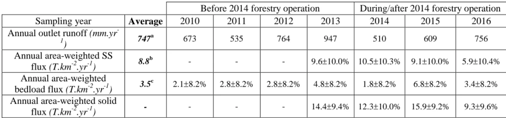
The main hydrological characteristics (annual open-field precipitation, runoff, and water quantity extracted for water supply) of the 7 years concerned by the bedload flux study (2010-2016) are summarized in Table 1.
The 7 studied years were highly hydrologically contrasted. With rainfalls exceeding the past 30-year mean annual precipitation by 20% and 21%, 2012 and 2013 were wet years. Conversely, 2011 and 2014 were rather dry years with precipitation deficits of 12% and 11%, respectively. In 2010, 2015, and 2016, the annual precipitation was close to the long-term average value (deviations less than 7%). For comparison, the annual runoff was particularly high in 2013 and low in 2014 (deviations of +34% and -30%, respectively). The ratio between the annual total runoff and annual precipitation followed this same trend (ratios of 0.65 and 0.46 for wet and dry years, respectively). These differences are mainly due to the frequency and intensity of snowmelt events (high frequency and intensity in 2013 and very low frequency and intensity in 2014). Actually, in the study site, snowmelt mainly occurs in the early and late winter and early spring when evapotranspiration is the lowest. In contrast, 2012 was characterized by a substantial amount of precipitation falling as thunderstorms, explaining a lower ratio than that for the year 2013, despite similar amounts of snow precipitation. In particular, stormy precipitation occurs in late spring or summer when evapotranspiration is high.
3.2. Impact of the hydrological regime on the solid export dynamics
The time series of processed SS concentration is shown in Fig. 3a, b, c, and d for the 4 years concerned by the high-frequency SS flux study (2013-2016). In this figure, a vertical gray dot line marks the beginning of each
Journal Pre-proof
flood sampled by the high-flow sampler. Among those flood events, a gray vertical arrow identified the long-lasting events sampled for more than one day (corresponding to events with a delayed-flow peak).
Among the flood events that occurred during the 4 studied years, 85 were collected with the high-flow sampler, including all the major long-lasting events. Some short events could not be sampled because the sampler was already filled by water from previous flood events. However, the majority and the variety of flood events are present in our processed dataset of SS concentrations. Among the 25 major events sampled, 14 correspond to widespread snowmelt at the catchment scale, 7 are due to significant thunderstorms inducing substantial rain intensities (maximum precipitation intensity of more than 5 mm in 10 min), and 4 are due to other major atmospheric disturbances providing large amounts of rain (more than 60 mm in a few days).
The highest SS concentrations were measured during thunderstorm events (for instance, on the afternoon of April 26, 2015), when the increase in stream discharge and energy was extremely rapid, inducing a quasi-simultaneous mobilization of particles of very different sizes at each point of the brook. In contrast, lower SS concentrations were measured during long-lasting events such as snowmelt (for instance, at the end of December 2012). Indeed, the slow increase in discharge during this type of event induced slow and successive suspension of the different sizes of particles at each point of the brook.
The mean SS concentration measured in the stream at the catchment outlet was 31 mg.L-1 for the 4 studied years. This concentration, ranging from 0 to 2.7 g.L-18.0%, showed significant variability. This substantial temporal variability in the SS concentration and SS flux is specific to small mountainous catchments (Maneux et al., 1999; Coynel et al., 2004; Mathys, 2006). The maximum SS concentration measured before the second recent forestry operation beginning in July 2014 was 0.61 g.L-18.0%, already underlining its strong impact on SS concentrations. The effects of forest management on SS exports are discussed in Sect. 3.3.2 and 3.3.4. The runoff-weighted mean SS concentration was 12.3 mg.L-1 for the 4 studied years, which is higher than the data previously published for the same catchment. Indeed, for the 6 hydrological years between 2005 and 2010, the weighted mean SS concentration was equal to 4.1 mg.L-1 (Viville et al., 2012). This difference can be explained by i) a lower frequency of the sampling before December 2012 (26 samples per year compared to approximately 700 samples per year in this study), leading to a less accurate estimation of the annual SS export flux (Phillips et al., 1999; Coynel et al., 2004; Moatar et al., 2006; Mano et al., 2009), ii) the lack of major forest harvesting, which could substantially disturb solid exports between 2005 and 2010 (Megahan and Kidd, 1972; Motha et al., 2003), and iii) the inter-annual variability in the solid exports.
Journal Pre-proof
The time series of fortnightly solid fluxes (SS and bedload) are shown in Fig. 4a, b, c, and d for the 4 years concerned by the high-frequency SS flux study (2013-2016). These solid fluxes are based on the processed SS concentration time series (SS flux - see Sect. 2.2.3 and 2.2.4) and the volume of fortnightly accumulated sediment (bedload flux - see Sect. 2.3.1 and 2.3.2).
For the 4 studied years, the mean solid fluxes exported fortnightly from the catchment were 0.27 T for the SS and 0.13 T for the bedload (for details on uncertainties of SS and bedload fluxes, see supplementary information B.1 and B.2). The fortnightly SS flux ranged from 0.0088 T15% (October 2016) to 2.8 T8.9% (December 2012) whereas the fortnightly bedload flux ranged from 0 to 0.98 T8.2% (October 2013). During the 4 studied years, within the 104 evaluated flux values, the fortnightly bedload flux equaled zero 36 times, that is, 35% of the time. Note that a bedload flux of less than 3 kg per fortnight is considered non-significant. The fortnights with negligible bedload flux correspond to low-water periods (mean stream discharge of 7.0 L.s-1) when brook competence is insufficient to transport its coarse sediments. Furthermore, the proportion of the fortnightly solid flux exported as bedload varied between 0% and 68% (January 2013). Solid fluxes and their partitioning between the bedload and SS showed large scatter in the case of the Strengbach catchment. The high proportions of bedload exported appear to be more prevalent at the end of long-lasting flood events when discharges have already significantly decreased (for example, the 3rd and 5th fortnights of the sampling year 2013 or the 4th and 7th fortnights of the sampling year 2015). Indeed, during significant long-lasting events, the proportion of the exported bedload first increases with rising fortnightly mean discharge and then often increases again with falling mean discharge at the end of the events. This first increase is due to the absence of bedload transport before the flood. The second increase can be due to the small amount of SS exported when the discharge decreases and the exportable SS supply strongly depletes, while the stream still has the hydraulic capacity to transport a non-negligible bedload amount. However, the low frequency of the bedload flux measurements compared to the short duration of most high-flow events in the small Strengbach catchment prevented us from going further in the study of the change in the solid flux portion exported as bedload over the studied years.
The periods contributing the most to the annual SS and bedload export fluxes are frequently the snowmelt periods and, more generally, the periods concerned by hydrological events with delayed-flow. The contribution of those events (see selected events in Fig. 2) to the solid exports is shown in Table 2 for the 4 years concerned by the high-frequency SS flux study (2013-2016).
Journal Pre-proof
Excluding the year 2014, the snowmelt events contributed between 39% and 57% to the annual SS flux and between 44% and 57% to the annual bedload flux. Over those same years, as a whole, the major events with delayed-flow contributed between 67% and 73% to the annual SS flux and between 69% and 83% to the annual bedload flux. With less than 10% of the solid exports during the snowmelt period, the SS and bedload transport dynamics of the year 2014 differ significantly from the solid transport dynamics of the other years. This can be explained by i) the small amount of snow precipitation (see Table 1), providing only minor snowmelt events, but mostly by ii) the forestry operation occurring in summer 2014, strongly disturbing the solid export dynamics. Year 2014 was also a dry year, including no major event with delayed-flow apart from the winter period. Without considering this year, the major events with delayed-flow contributed, on average, 70% of the annual SS flux and 75% of the annual bedload flux, while the period concerned by those events constituted, on average, only 37% of the year. In particular, the snowmelt events are responsible for carrying out, on average, half of the annual erosion flux. This high contribution of snowmelt events to the annual solid fluxes may seem surprising for a middle-mountain catchment with a mean of only 19% of the precipitation falling as snow.
This highlights the strong role of events with delayed-flow in the solid export dynamics of the Strengbach catchment. Indeed, as mentioned in Sect. 3.1.1, the delayed-flow events generate much more runoff than the quick-flow events due to i) similar peak discharge, ii) the high discharge mean duration of the flood peak being disproportionately larger for delayed flows than for quick flows, and iii) the non-negligible frequency of occurrence of the delayed-flow events. Even if the maximum SS concentration is significantly larger during the major quick-flow events due to a faster increase in the discharge, the total SS flux exported during this type of event is unlikely to reach the SS flux exported during the major delayed-flow events. Indeed, larger SS concentrations during quick-flow events do not compensate for the larger water fluxes at the outlet caused by delayed-flow events. As an illustration, similar discharges were achieved during 2 flood events in spring 2015. The quick-flow event of the afternoon of April 26 was responsible for exporting 0.25 T of SS, while the next delayed-flow event occurring a few days later between April 30 and May 13 generated a 1.0 T SS export. The SS exports were 4 times larger for the delayed-flow event than for the quick-flow event despite higher peak discharge during the quick-flow event and the lower amount of SS immediately exportable by the delayed-flow event due to the numerous flood events of the previous days.
The contribution of the delayed-flow events to the annual solid fluxes was greater for the bedload than for the SS. Indeed, if an SS transport subsisted during low-water periods, no bedload transport was detectable at
Journal Pre-proof
the same time at the Strengbach catchment outlet. Furthermore, except for large thunderstorm floods (less than 10 events during the studied period), the bedload transport during quick-flow events was unquantifiable because it was too weak while the SS flux regularly reached approximately 50 kg for the same events. This difference in the solid export dynamics mainly exists because i) the stream water needs to have sufficient hydraulic energy for carrying the coarse sediments, ii) the mean motion speed is much lower for the bedload than for the SS, and iii) the exportable supply is much more limited for the SS than for the bedload at any given time.
For the Strengbach catchment, the solid export dynamics are mainly driven by the dynamics of the delayed-flow events, which are often due to snowmelt. This type of hydrological functioning is unusual. Indeed, for most of the studied catchments, a large portion of the annual SS flux is carried during some major short-storm events (Coynel et al., 2004; Moatar et al., 2006; Mano et al., 2009; Duvert et al., 2011). However, for catchments with heavy snowfalls, the amount of sediment carried during the snowmelt period can be significant. Thus, for the Ferrand and Romanche watersheds (France), respectively, 38% and 31% of the annual SS flux is transferred during no-rainfall days in the period of snowmelt and ice melt (Mano et al., 2009). Furthermore, for the Lake Tahoe forested watershed (Nevada) where 90% of the annual precipitation falls as snow, the greatest SS fluxes are measured during the snowmelt period (Langlois et al., 2005).
3.3. Impact of the forest harvesting operations on the solid fluxes
3.3.1. Description of the forest harvesting operations
In May-June 2012 and July-August 2014, two forestry operation phases occurred in the lower part of the Strengbach catchment (see Fig. 1). The concerned plots were entirely planted with mature spruces from 40 to 52 years old. The forestry operations consisted of mechanized clear-cutting on steep plots (mean slope of 38%). A single-grip harvester carried out the tree delimbing at the felling place. Then, a forwarder carried the logs to the nearest forest road, which involved the implementation of skid trails.
In the 2012 forestry operation, spruces within 15 m of the stream were not cut, and soil close to the stream was never disturbed as in the case of tree harvesting with the preservation of riparian buffers. Due to the log extraction using the forest road located at the top of the plots, there was no forestry machine traffic in the brook and thus no disturbance of the stream channel.
Journal Pre-proof
In contrast, in the 2014 forestry operation, all trees, even those located close to the stream, were cut using forestry machines. As a result, the forest floor adjacent to the stream was significantly disturbed, including a complete bare soil exposure over a distance of approximately 150 m along the watercourse. Two crossings were also implemented to allow machine traffic in the stream, directly connecting the skid trail network to the stream channel. Due to the log extraction using the forest road located at the bottom of the plots across the brook, the crossings were used very frequently. Those stream crossings included a crossing located close to the catchment outlet (80 m from the outlet). In this last forestry operation, the skid trails created in 2012 were reused.
During the two forestry operations in the Strengbach catchment, no effort was made to control the implementation of skid trails and stream crossings, which were located and designed by loggers. Thus, no watercourse protection measures (for example, well-designed bridges or culverts to cross the stream, branch mats, or open-top culverts for skid trails) were implemented to mitigate anthropogenic sediment delivery to the brook. The crossings consisted of some small unsaleable logs placed longitudinally in the stream bed, forcing stream water to leave the stream bed to bypass the logs. Only bare soil covered the skid trails, and the slopes of their sections immediately adjacent to the log crossings were often steep (slope average was 17% with a minimum of 10% and maximum of 24%). Furthermore, at the completion of the 2014 forestry operation, logs constituting the crossings were removed from the stream channel. At the end of all forestry operations, even if the cutting residues (i.e., branches, twigs, and needles) were left on site to allow them to degrade naturally, mainly bare soil covered the deforested areas.
The area affected by all the forestry operations was relatively small and corresponded to less than 5% of the catchment area (2.3% for each forestry operation). Furthermore, the total area of the skid trails was comparatively large and accounted for 24% of the catchment areas deforested in 2012 and 2014.
In detail, the 2014 forestry operation included the following major steps: July 3 - implementation of stream crossings and major skid trails; July 7-August 8 - tree harvesting and extension of the skid trails; and August 11 - completion of the forestry operation, including the removal of logs constituting the stream crossings and the end of all machine traffic outside the few forest roads in the study site located far from the brook.
3.3.2. Impact of the 2012 forestry operation on the solid fluxes
Journal Pre-proof
Journal Pre-proof
When forestry operations are implemented near perennial or seasonal streams without any disturbance of the stream bed and the soil surface within their riparian areas (for example, in accordance with forestry best management practices (BMPs; Cristan et al., 2016), the solid fluxes often remain minimally affected (Wynn et al., 2000; Lakel et al., 2010; Nisbet et al., 2002; Clinton, 2011; Witt et al., 2016; Hatten et al., 2018). However, indirectly, in the case of large harvested areas, the erosion flux can significantly increase because of the reduction in evapotranspiration resulting in an increase in the outlet water flux and thus of the solid fluxes (Rodgers et al., 2011; Webb et al., 2012). In view of the features of the spring 2012 forestry operation - a small harvested area and no disturbance of the stream bed and its riparian zone - it is reasonable to assume that this forest harvesting had no impact on the solid exports at the catchment scale. In addition, in the Strengbach catchment, following the 2012 forestry operation, no sediment delivery pathway, such as a gully or sediment plume (and then no direct connection), was detected between the harvested areas or skid trails and the watercourse.
Furthermore, the high-frequency study of the SS flux exported from this catchment using automatic sampling began in December 2012, so the spring 2012 forestry operation impact cannot be studied using this SS flux estimation method. However, since 2005, SS flux can be estimated based on low-frequency manual sampling (26 samples per year; Viville et al., 2012). Due to the small number of considered samples, this former flux estimation method remains imprecise. However, it is the only one suitable for an evaluation of the impact of the 2012 forestry operation. Fig. 5 shows the annual solid fluxes (SS and bedload) between 2005 and 2016 with SS flux estimation based on manual samples.
In this erosion flux time series, no significant increase in the SS and bedload fluxes was observed for the sampling year 2012. Therefore, the fluxes of the years prior to the summer 2014 can be considered undisturbed fluxes.
3.3.3. Undisturbed solid fluxes
The annual solid fluxes are shown in Table 3 for 7 years for the bedload (2010-2016) and for 4 years for the SS (2013-2016). Notice that only SS flux estimations based on high-frequency sampling are presented in this table.
Journal Pre-proof
For the entire study period, the area-weighted annual solid fluxes exported from the catchment show an important variability ranging from 5.9 T.km-2.yr-110.4% to 10.5 T.km-2.yr-110.3% with a mean of 8.8 T.km-2.yr-1 for the SS, and 1.8 T.km-2.yr-18.2% to 6.8 T.km-2.yr-18.2% with a mean of 3.5 T.km-2.yr-1 for the bedload.
Before the summer 2014 forestry operation, the area-weighted annual solid flux of our study site was 14.4 T.km-2.yr-19.4% (estimated for the sampling year 2013). Comparison with the mean values of the area-weighted annual erosion flux reported for various granitoid catchments shows that the solid flux exported from the Strengbach catchment is quite low. Only approximately 10 solid flux values lower than the erosion flux of our study site have been observed (Martin and Hornbeck, 1994; Martin et al., 2000; Millot et al., 2002; Riebe et al., 2004; West et al., 2005). The values of those fluxes range between 3 T.km-2.yr-1 and 14 T.km-2.yr-1. Most of the erosion flux values reported are far more important than the solid flux exported from our study site (Bhutiyani, 2000; Millot et al., 2002; Riebe et al., 2001 and 2004; West et al., 2005; Gabet et al., 2010; Zhang et al., 2017; Dannhaus et al., 2018). The values of those fluxes range between 15 T.km-2.yr-1 and 1540 T.km-2.yr-1. Except for strongly anthropogenically impacted catchments, basins with very high values of erosion flux are mostly high mountainous catchments with areas covered by glaciers and/or very steep slopes prone to landslides (Bhutiyani, 2000; Gabet et al., 2010) or humid tropical climate catchments with large amounts of precipitation (West et al., 2005). The relatively low solid flux exported from the Strengbach catchment before the 2014 forestry operation can be explained by the lack of surface runoff during rainfall events (except on the few forest roads), lack of very steep slopes, an almost total forest cover, mean-scale annual precipitation, very few hydrological events with extreme rainfall intensity, and the absence of major anthropogenic disturbance at the basin scale. The absence of very steep slopes and the large forest cover limit landslide hazards in this middle-mountain catchment.
A wide range of values for the portion of the annual solid flux exported as bedload can be found in the literature. Long-term average partitioning is a function of the catchment area and its geology and perhaps of the fraction of the catchment covered by glaciers or forests (Turowski et al., 2010). Thus, the portion of bedload exported generally increases with decreasing drainage area and increasing bedrock strength. In the literature, a few times, a portion of the annual solid flux exported as bedload of approximately 10% was assumed or quantified (Grant and Wolff, 1991; Meybeck et al., 2003; Coynel et al., 2004; Hancock et al., 2017). Low values of this proportion, on the order of 1%, have been measured in some gravel-bed rivers draining very large catchments (McLean et al., 1999; Vericat and Batalla, 2006). Numerous high values of this proportion, between 23% and 33%, have been observed (Grant and Wolff, 1991; Mathys, 2006; Schmidt and Morche, 2006; Lenzi et al.,
Journal Pre-proof
2003; Pratt-Sitaula et al., 2007; Gabet et al., 2008 and 2010). Higher values of this proportion are quite rare except in the case of small catchments (Mathys, 2006; Turowski et al., 2010). It is interesting to note that a very high value of this proportion (i.e., 80%) was found for the small granitic catchments of the Hubbard Brook experimental forest in the United States (Martin and Hornbeck, 1994; Martin et al., 2000). For the small granitic Strengbach catchment, solid exports are dominated by SS transport, but bedload transport is not negligible with an annual solid flux divided into 67% SS and 33% bedload before the 2014 forestry operation.
The annual solid flux estimated for the Strengbach catchment is also higher than the annual erosion flux previously published for the same catchment. Indeed, for the hydrological year 2010, an annual solid flux of 5.0 T.km-2.yr-120% was determined (Viville et al., 2012). This difference can be explained by a higher uncertainty in the estimation of the annual SS export flux before December 2012 and by the inter-annual variability in solid exports. Large natural variability in the annual bedload flux has already been observed for the catchments of the Hubbard Brook experimental forest with area-weighted flux ranging from 0.13 T.km-2.yr-1 to 12 T.km-2.yr-1 for one of the undisturbed basins (Martin et al., 2000). For the Strengbach catchment, before the 2014 forestry operation, the area-weighted annual flux of the bedload ranged from 2.1 T.km-2.yr-18.2% to 4.8 T.km-2.yr-18.2%, showing a significantly smaller variability than in the case of the undisturbed Hubbard Brook basin. Furthermore, over this period, the highest annual bedload flux was measured for the sampling year 2013, which also has the highest annual outlet water flux (see Table 1). For the Strengbach catchment, the year-to-year variability in the bedload flux appears to be at least partially linked to the inter-annual variability in the outlet runoff. Before the 2014 forestry operation perturbation, the correlation of the annual bedload flux with the annual outlet runoff gave an r² coefficient value of 0.61. It seems that the annual solid flux is controlled by the annual outlet runoff, as already observed by Jordan (2006) for two basins located in British Columbia. Similarly, annual chemical fluxes at the Strengbach catchment outlet since 1987 are also significantly correlated with the annual outlet runoff, with r2 ranging from 0.65 to 1 (Pierret et al., 2018). Between 2010 and 2016, the annual outlet runoff ranged from 510 mm.yr-1 to 947 mm.yr-1, giving a ratio between extreme water fluxes of almost 2. To isolate the 2014 forestry operation as a controlling factor, the annual solid fluxes were normalized according to the annual outlet water flux (see Fig. 6) as already proposed by Gabet et al. (2010).
3.3.4. Impact of the 2014 forestry operation on the solid fluxes
Journal Pre-proof
Journal Pre-proof
Fig. 6 shows the ratio between the annual solid fluxes and the annual outlet water flux for the 7 years concerned by the bedload flux study, helping to quantify the impact of the summer 2014 forestry operation on the annual export fluxes. Before this forestry operation, the ratio between the annual bedload flux and the annual outlet runoff was significantly less variable than the annual bedload flux (see Fig. 5).
Starting in the first days of July and ending mid-August 2014, the forestry operation resulted in a significant and quasi-immediate impact on the SS concentration (see Fig. 3) and fortnightly SS flux (see Fig. 4).
Outside any high-flow period, in the 16th fortnight of the sampling year 2014 (July 9-July 22), the mean SS concentration of the stream was 129 mg.L-1 whereas in the 14th fortnight (June 10-June 24), the mean SS concentration was 6.2 mg.L-1. The mean concentration in the samples collected before the beginning of the 2014 forestry operation was in the range of the SS concentrations usually measured at the Strengbach catchment outlet during summer low-water periods. The highest impact of the forestry operation on the stream water quality occurred when tree harvesting was ongoing with measured SS concentrations up to 1.18 g.L-18.0% in low-water conditions. This maximum concentration corresponds to approximately 190 times the mean SS concentration measured in the stream before the forestry operation began, but it was also 2 times the maximum SS concentration ever measured before July 2014 (i.e., 0.61 g.L-18.0% measured on August 27, 2013), showing the large impact of the forestry operation on the low-water SS concentrations. Unexpectedly, we did not detect any impact of stream crossing implementation on July 3 with a stream SS concentration varying between 5.2 mg.L-111.2% on July 2 at 5 p.m., 6.3 mg.L-111.2% on July 3 at 9 a.m., and 2.5 mg.L-111.2% on July 4 at 1 a.m. Between the 17th (July 22-August 5) and 20th (September 2-September 16) fortnights of the sampling year 2014, the mean SS concentration outside any high-flow period decreased from 53 mg.L-1 to 7.5 mg.L-1, converging toward the concentration level measured in the stream before the forestry operation began. Thereafter, we no longer measured fortnightly mean concentrations under low-water conditions of more than 7.6 mg.L-1. Assuming experimental uncertainty, we can consider that the 19th (August 19-September 2) fortnight of the sampling year 2014 was the last period where the SS concentration outside flood events was disturbed by the forestry operation. Thus, a month after the completion of the 2014 forestry operation, its impact on stream SS concentration was no longer detectable under low-water conditions. Furthermore, during the tree harvesting period, outside flood events, the mean SS concentrations of the water samples collected at 9 a.m., 5 p.m., and 1 a.m. were 145 mg.L-1, 64 mg.L-1, and 27 mg.L-1, respectively, reflecting the strong immediate but rapidly
Journal Pre-proof
decreasing impact on SS transport of the machine traffic on the skid trails and stream crossings during the logger working days (typically 7 a.m.-3 p.m.).
The impact of the forestry operation on SS exports was also significant during flood events with SS concentrations up to 2.7 g.L-18.0% measured for a modest stream discharge of 45 L.s-1 on July 25, 2014, at 2:51 p.m. This concentration represents 4 times the maximum SS concentration ever measured in the stream before July 2014 for a range of sampled discharges up to 202 L.s-1. If outside the flood periods, only a month after completion of the forestry operation, the stream SS concentration seems to have already recovered this level before the anthropogenic disturbance; this was not the case during high-flow periods. For example, during the 23rd fortnight of the sampling year 2014 (October 14-October 28), two middle-scale flood events generated much larger SS fluxes than expected. In comparison, during the 14th fortnight of the sampling year 2016 (June 7-June 21), two similar high-flow events were responsible for the export of an 85% lower fortnightly SS flux than that in the 23rd fortnight. Based on the knowledge of the solid export dynamics during similar hydrological events prior to the 2014 tree harvesting operation, it was possible to determine the last hydrological event impacted by this forestry work and to estimate the extent of its impact on the solid fluxes. The last certain impact on SS exports occurred during middle-scale snowmelt events from late December 2014 to late January 2015. A stronger impact of forestry operations on the SS fluxes during the snowmelt months has already been reported by Karwan et al. (2007). Thus, 6 months after completion of the forestry operation, following the first snowmelt events of the next sampling year, the tree harvesting impact on the SS flux was no longer noticeable in high-flow periods. This longer-term impact of the forestry operation during high-flow events resulted in larger annual SS fluxes for not only the year of the works but also the next year (see Fig. 6). For the Strengbach catchment, a 5-month gap existed between the recovery times in the low-water and high-flow conditions. Indeed, at the completion of the forestry operation, a large amount of anthropogenic SS had been introduced into the Strengbach watercourse mainly due to machine traffic on stream crossings during adverse weather conditions. In low-water periods, except for the natural SS flux, only the amount of anthropogenic SS introduced during the forestry work could be exported from the catchment. Once this amount was exhausted, the SS flux returned to an unaffected value. In our study, this exhaustion was relatively rapid due to the numerous successive flood events occurring between mid-July and late August 2014. During rain events, due to surface runoff on the skid trails, new amounts of anthropogenic SS were introduced into the watercourse. Once delivered to the short Strengbach stream, those anthropogenic SS were quickly exported outside the catchment, likely at the scale of a unique hydrological event.
Journal Pre-proof
The 2014 forestry operation in the Strengbach catchment led to approximately 5 to 6 times larger fortnightly SS fluxes than that expected when the works were ongoing and to approximately 2 and 1.5 times larger annually exported SS fluxes for the sampling years 2014 and 2015, respectively. Overall, a post-logging recovery time of 6 months can be considered for SS exports at the Strengbach catchment scale.
No clear influence of the forest harvesting operation on the fortnightly bedload flux could be observed during the sampling year 2014, including when the works were ongoing. The impact on the bedload flux was not significant at the scale of this year. Conversely, during the following sampling year, the annual bedload flux was approximately 2 times larger than expected, reflecting a delay in the tree harvesting impact on the coarse sediment exports. At the fortnight scale, we clearly observed a notable impact during all events with a delayed-flow peak (snowmelt events and spring events due to large amounts of rain) between late December 2014 and mid-May 2015. This type of delayed impact of forest harvesting on bedload exports of a catchment has already been reported by Martin and Hornbeck (1994). Indeed, if SS transport is continuous and quick, bedload transport is discontinuous and slow, and time is needed to carry anthropogenic source coarse sediments from their areas of production and introduction into the watercourse to the catchment outlet. In addition, in our study, when the works were ongoing, the trapping of sediment upstream of the small logs constituting stream crossings could restrict bedload transport along the watercourse (Ryan et al., 2014). The smaller transport speed for coarse sediments leads to longer recovery time for bedload exports than for SS exports. Quicker recovery to pre-logging flux for SS than for bedload was already observed by Grant and Wolff (1991). A post-logging recovery time of 10 months can be considered for bedload exports at the Strengbach catchment scale.
Overall, a post-logging recovery time of approximately 10 months can be assumed for the solid exports following the 2014 forestry operation in the Strengbach catchment. This recovery time (and also the extent of the solid export disturbance) relies not only on forestry operation conditions and on topographical and geological characteristics of the catchment but also on site hydrology during and after the tree harvesting (i.e., soil moisture, number and duration of flood events, and discharges reached during high-flow events).
Furthermore, we notice that the annual SS and bedload fluxes in the sampling years with an assumed non-disturbed solid transport (i.e., 2013 and 2016) are on the same order of magnitude (see Table 3). However, the solid exports in the sampling year 2016 are significantly smaller than the erosion flux in the sampling year 2013, which is consistent with a smaller annual outlet runoff in the last year of this study. In addition, the proportion of the annual solid flux exported as bedload is also very close for those two years; namely, a solid flux