HAL Id: hal-01276849
https://hal.univ-lorraine.fr/hal-01276849
Submitted on 4 Mar 2016
HAL is a multi-disciplinary open access
archive for the deposit and dissemination of sci-entific research documents, whether they are pub-lished or not. The documents may come from teaching and research institutions in France or abroad, or from public or private research centers.
L’archive ouverte pluridisciplinaire HAL, est destinée au dépôt et à la diffusion de documents scientifiques de niveau recherche, publiés ou non, émanant des établissements d’enseignement et de recherche français ou étrangers, des laboratoires publics ou privés.
Elements for measuring the complexity of 3D structural
models: Connectivity and geometry
Jeanne Pellerin, Guillaume Caumon, Charline Julio, Pablo Mejia-Herrera,
Arnaud Botella
To cite this version:
Jeanne Pellerin, Guillaume Caumon, Charline Julio, Pablo Mejia-Herrera, Arnaud Botella. Elements for measuring the complexity of 3D structural models: Connectivity and geometry. Computers & Geosciences, Elsevier, 2015, 76, pp.130-140. �10.1016/j.cageo.2015.01.002�. �hal-01276849�
Elements for measuring the complexity of 3D structural models:
connectivity and geometry
Jeanne Pellerina,b, Guillaume Caumona, Charline Julioa, Pablo Mejia-Herreraa, Arnaud Botellaa,b
aGeoressources (UMR 7359), Universit´e de Lorraine-ENSG, TSA 70605, 54518 Vandoeuvre-l`es-Nancy Cedex,
France
bProject ALICE, INRIA Nancy Grand Est, 615 rue du jardin botanique, 54600 Villers-l`es-Nancy, France
Abstract
The reliable modeling of three-dimensional complex geological structures can have a major im-pact on forecasting and managing natural resources and on predicting seismic and geomechanical hazards. However, the qualification of a model as structurally complex is often qualitative and subjective making the comparison of the capabilities and performances of various geomodeling methods or software difficult. In this paper, we consider the notion of structural complexity from a geometrical point of view and argue that it can be characterized using general metrics computed on three-dimensional sealed structural models. We propose global and local measures of the con-nectivity and of the geometry of the model components and show how they permit to classify nine 3D synthetic structural models. Depending on the complexity elements favored the classification varies. The models we introduce could be used as benchmark models for geomodeling algorithms. Keywords: Local measures, Global measures, Complexity elements, Geomodeling, Surface model
1. Introduction
The terms structurally complex, as opposed to structurally simple, are widely used in the geosciences community to characterize the features of a geological domain. Indeed, understanding and predicting the behavior of complex geological structures can be a difficult task that often has a direct impact on the challenges, costs, and risks associated with the discovery and exploitation of natural resources (Dromgoole and Speers, 1997; Trubetskoy et al., 2012; Jolley et al., 2007). Moreover, the exploration and the management of future resources require to study more and more structurally complex areas (Jolley et al., 2007). This makes the adequate representation of geological structures in 3D subsurface models a very important aspect in producing reliable forecasts. However, managing structural complexity in 3D modeling raises a several questions because a model is, by definition, an idealized and simplified vision of reality. How far should a model represent the complexity of the actual natural structures? At what scale? What is exactly meant when a theory, method or algorithm is claimed to address structurally complex geological domains? The term complex is indeed generally used in a qualitative and subjective way depending
Please cite this paper as: J. Pellerin, G. Caumon, C. Julio, P. Mejia-Herrera, and A. Botella, “Elements for measuring the complexity of 3D structural models: Connectivity and geometry,”
on the person making that statement, on his/her education and experience, on the means at his/her disposal, and on the purpose of his/her work.
In this paper, we propose to analyze the complexity of 3D sealed structural models by describing and quantifying model elements which contribute to the geometrical complexity of the geological structures. A complexity that has an impact on several geomodeling tasks, from data processing to numerical simulation. We propose elementary measures of the geometry and of the connectivity (topology) of 3D structural models that are represented by a set of triangulated surfaces delimiting the different rock volumes. These surfaces may be obtained from subsurface data using either ex-plicit surface-based structural modeling (seeCaumon et al.(2009) for a review) or implicit surface modeling methods (Frank et al., 2007;Calcagno et al., 2008; Caumon et al., 2013; Hillier et al.,
2014). The proposed measures only relate to the geometry of the structures that are represented in the model and do not include information about facies and rock properties. Their primary goal is to evaluate the relative complexity of several structural models, and to identify the areas in a model which are likely to raise challenges for further modeling tasks such as volumetric gridding. For example, when geological models are found to be too detailed as compared to the time require-ments or capabilities of physical simulators (e.g., Farmer, 2005), their resolution can be reduced through simplification and upscaling of geological structures (Bourbiaux et al., 2002; Mustapha
and Mustapha, 2007; Pellerin et al., 2014). The measures we propose could help assessing how
much a detailed initial model has been simplified and evaluating the method that was used. A first step toward quantifying structural complexity is to agree on a qualitative understanding of the term. Therefore, we first discuss this notion in a synthetic literature review in various disciplines (Sect.2). Then, after describing elements contributing to the geometrical and topological complexity of structural models (Sect.3), we propose global and local measures of this complexity (Sect. 4), evaluate them on a set of nine synthetic models1 that display typical challenges for geomodeling, and show how the measures can be used to classify these models (Sect.6).
2. Views on structural complexity and related work
Complexity is a research area in itself which has implications in systems science, biology, social sciences, economy, etc. (Gell-Mann, 1995; Manson, 2001). In this paper, we are interested in complexity as a measure of the difficulty to describe the geometry of geological structures. We are working directly on the surface descriptions, to ensure that the complexity analysis relates to the actual structures and filters out data and interpretation inconsistencies which are commonly observed.
In structural geology, complexity primarily relates to the intensity and localization of rock de-formations and to the succession of tectonic, sedimentary, diagenetic, igneous and metamorphic processes. Conceptual geological models typically aim at generating a consistent succession of events which can explain observations and translate them into likely geometric objects. For in-stance, the presence of tectonic inversions (e.g., inverse reactivation of normal faults in compressive contexts) is often seen as a source of structural complexity, see Sassi et al. (1993). Our focus in this paper is not to characterize the complexity of the tectono-stratigraphic history and processes per se but to characterize their impact on the 3D structures. Chiaraluce (2012), among others,
shares this view and mentions the presence of fault splays, branches, and segmented faults as ele-ments contributing to the complexity of a fault system. These configurations are captured by the geometry and connectivity measures defined in Sect. 4.
Another view on structural complexity is conveyed by geoscientists interested in physical pro-cesses in the subsurface. For instance,Jolley et al.(2007) define structurally complex reservoirs as reservoirs “in which fault array and fracture networks, in particular, exert an over-riding control on petroleum trapping and production behavior”. Matthai et al. (2007) mention the sharp variations of the permeability field often associated to geological structures and the difficulty to represent and discretize these structures at several scales. In seismology, Ravaut et al. (2004) define com-plex structures as “characterized by strong lateral variations in the velocity field”. From this point of view, structures are important because they partly control the spatial layout of petrophysical heterogeneities. They must then be accounted for in the grids on which numerical simulations are run. However, to obtain precise and reliable results in reasonable time, model resolution should be adequate, and the grid should represent the structures precisely enough while respecting a set of quality criteria on the number, aspect, type, and size of its elements. This is a challenge for all gridding methods, particularly when the model contains geometrical features which dimensions are smaller than the desired mesh size (Quadros et al.,2004;White et al.,2005). The gridding effort is then a significant consequence of structural complexity. The measures we propose help identifying the zones which can be particularly difficult to mesh.
In geosciences, several papers propose model complexity evaluations using a subdivision of the models into different cells. Andrle(1996) uses radius-varying circles to compute a resolution-adapted angle measure and evaluate the complexity of geomorphic lines. Lindsay et al. (2013a) propose a local connectivity complexity measure for models represented as regular Cartesian grids. For each cell, the number of stratigraphic layers sampled by the cell and its adjacent cells is determined, and the average value of this local measure is computed over the model. This local counting principle is also used by box-counting methods to compute fractal dimension (Kruhl,
2013). The neighborhoods measures proposed in Sect. 4 follow this idea of measuring locally the model complexity.
In other modeling fields using a similar 3D representations, several papers propose global eval-uations of model complexity (Rossignac,2005;Sukumar et al.,2008;White et al.,2005;Quadros
et al.,2004). In geometric modeling, Rossignac (2005) discusses several aspects which contribute
to the complexity of 3D models and influence design, implementation, stability, and performance of 3D modeling systems. We will mainly consider topological and morphological complexity (in Rossignac’s terms) and adapt these to geological features. In visualization,Sukumar et al. (2008) identify surface variations, symmetry, number of parts, details and topology as the six aspects that influence visual shape complexity. To compute a mesh sizing function,Quadros et al. (2004) identify the small geometrical characteristics in a model from the proximity between two surfaces (distance to medial surface), the proximity between two lines (distance to medial axis), surface curvature, length and curvature of the surface boundary lines. We propose measures taking into account similar distances in Sect.4.
3. Sources of complexity
In this section, we propose a short analysis showing how the number of geological features (layers, horizons, faults, etc.) and their relationships contribute to the geometrical and topological
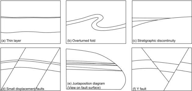
Figure 1: Cross-section views of some sources of complexity in geological structural models.
complexities of a 3D structural model, and impact on several tasks of the geomodeling workflow, from data processing to numerical simulation.
3.1. Number of geological features
The complexity of a model depends on the number of continuous layers (or rock units) it contains, on the number of discontinuities affecting these layers, and on the geometry of these layers and discontinuities. During surface model building, the consistency of each of these layers must be checked, having a direct impact on modeling time (Caumon et al., 2009). The number of volumetric regions (one per layer and per fault block) also often determines the number of stationary regions to be used in petrophysical models, hence the corresponding increase in effort needed for geostatistical inference and modeling. Because each feature may correspond to localized petrophysical contrasts and induce compartmentalization of the domain, it often has a first-order impact on flow and geophysical processes.
3.2. Interactions between features
The spatial distribution of geological features inside the model has a direct impact on the modeling, gridding, and simulation steps. It is linked to the geometry of the features and to to the intersections between the model layers, faults, and unconformities. The least complex elements are those that are the easiest to remove and to modify because they have few interactions with other model elements. Conversely the most complex elements potentially intersect a large number of elements and are subsequently more difficult to remove or modify due to cascading effects on their neighbors.
3.2.1. Conformable layers
Conformable layers may be challenging if one of them is locally very thin (Fig. 1a), because layer validity (no intersection between top and bottom horizons) is then generally more difficult to check. Abrupt thickness variations may also raise difficulties when building a model by interpolating scarce data (Mallet, 2002). Additionally, layer thickness variations can introduce difficulties in
discretization of fluid transport problems due to the juxtaposition of relatively large and small volumes. Deformation, such as folding, may affect layer thickness and horizon curvature. Some structures like overturned and recumbent folds (Fig.1b) are more complex to represent than gentle folds, because they cannot be represented as single value height fields, which can be problematic for some applications (Mallet,2002;Farmer,2005).
3.2.2. Stratigraphic unconformities
Vertical relationships between layers controlled by unconformities are very common in strati-graphic domains which host most of the world’s hydrocarbon reservoirs and aquifers.. Due to their economic importance, significant efforts have been made in earth modeling methods to handle such configurations (Mallet,2002;Farmer,2005;Caumon and Mallet,2006;Calcagno et al.,2008;
Cau-mon et al.,2013). They often involve thin layers and low angles between horizons (Fig. 1c) which
are difficult to characterize from observations and involve more modeling operations and quality controls than conformable stratigraphic sequences. These low angles and thin layers are very chal-lenging when gridding the model, especially for unstructured mesh generation (e.g. Mustapha and
Mustapha (2007);Durand-Riard et al.(2010); Pellerin et al.(2014)).
3.2.3. Faults
Faults are discontinuities inducing a displacement of the rock units localized along a surface (Fig. 1d). They are often difficult to characterize from subsurface data and introduce significant complexity due to their connectivity, shape, and specific properties (Jolley et al., 2007). In all faulted configurations, the presence of possibly noisy data calls for a quality control step to validate the fault slip, for instance by analyzing the fault cutoff lines through an Allan (or juxtaposition) diagram (Fig.1e) (Groshong,2006). Juxtaposition is also very important for flow purposes because it leads to strong non-linearities of the flow response to small geometric perturbations (Jolley
et al., 2007; Tavassoli et al., 2005). Intersections at small angles of fault-horizons contact lines
may introduce difficulties in mapping of layer juxtaposition and gridding, and can affect fault transmissibility. Blind faults raise similar challenges because they stop in the model and the nil displacement at their tips is linked to very small angles between fault-horizon contacts in the Allan diagram (Fig.1e).
When considering a fault network, the total complexity is more than the combination of the individual fault complexities. It also depends on the variability of the fault orientations and on the number, angle, length, and orientation of branch lines. These features have a major impact on the approximations required for griding. For example, horizontal branch lines between faults (Y-shaped configurations) (Fig. 1f) or strong variations of the orientations and dip of faults can prevent the easy representation of the model by the extrusion of a cross-section, or the gridding with pillar grids (Farmer,2005;Caumon and Mallet,2006).
4. Measures
4.1. Structural model components
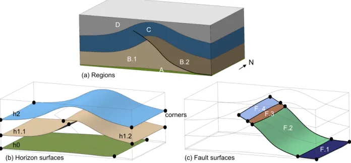
In this paper, we consider volumetric models described by their boundary surfaces (also called B-Rep models). In geological models, these surfaces are of three main type: horizons (delimiting layers), discontinuities (faults, erosion surfaces, etc.), and surfaces delimiting the volume of interest. They define the volumetric regions of the model (Fig.2a). They are delimited by their boundary lines that are either at the intersection of several surfaces (full lines on Fig.2c), or on the boundary
Figure 2: Elements of a structural model.
of a unique surface (dashed line on Fig. 2c). These lines have two extremities called corners (Fig. 2b; some boundary line may be closed, they have no extremity). We consider independently the connected components of the model geological features (layer, fault, horizon, fault-fault contact, etc.). Each region, surface, line, or corner corresponds to a unique geological feature, while a geological feature may be described by several regions, surfaces, lines, or corners. For example, the model on Figure 2 is constituted of four layers (A, B, C, D) delimited by three horizons (h0, h1, h2) and cut by one fault F. Layer B is cut in two regions: B.1 and B.2. Horizon h1 has two surfaces and the fault has four surfaces numbered from 1 to 4, each being delimited by four lines, themselves delimited by two corners.
From this definition of three-dimensional structural models we suggest to evaluate the model complexity C as a sum of the complexity of its components
C= CRegions+ CS ur f aces+ CLines+ CCorners (1)
To evaluate the complexity of the components we propose local and global measures of their connectivity (topology) and geometry.
4.2. Global complexity measures
We propose three global measures evaluating the complexity of one model. The first counts the number of elements of the model (regions, surfaces, lines, and corners) excluding the ones defining the volume of interest, and giving the same weight to each element.
C1= NRegions+ NS ur f aces+ NLines+ NCorners (2)
We saw in the previous section that sizes, thicknesses, curvatures and angles are four impor-tant points of the geometrical complexity of structural models. We then propose to compute the geometrical complexity of each element as the sum of four measures characterizing (1) its size Cs;
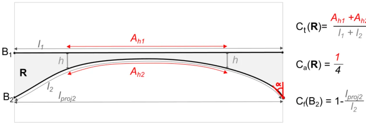
Figure 3: Geometrical measure computations in the plane. Thickness measure Ct and angle measure Ca for a region
R and shape measure Cf for one of its boundaries B2.
(2) its shape Cf; (3) its thickness Ct; and (4) its angles Ca, the sum over all model elements gives
a second global complexity measure:
C2=
X
e∈ {Regions ∪ S ur f aces ∪ Lines}Cs(e)+ Cf(e)+ Ct(e)+ Ca(e) (3)
Corners are not explicitly taken into account in this measure, but have an indirect impact on the values obtained for the lines and surfaces. Each of the elementary measures is chosen so that it has values between 0 and 1. Cs(e) compares the size of component e (a line length, a surface area,
or a region volume) to a characteristic size h given by the user. Cs(e)=
(
0 i f size(e) > hd 1 else
The thickness complexity Ct relates to the thin features of the element (Fig. 3). It is defined
by considering the proximity of a boundary point with the other boundaries of the element. More formally, consider a boundary point p ∈ ∂e; this point is located on an element e0 ∈ ∂e. Let the thickness t(p) denote the shortest distance between p and ∂e\e0. Then, Ct(e) is defined as the
percentage of the boundary of e for which the thickness is smaller than a given characteristic size: Ct(e)=
(
0 for lines
Ah
size(∂e) for regions and surfaces
where d is the element dimension (0 for corners, 1 for lines, 2 for surfaces, 3 for regions). Ah the
extension of the zone where t(p) < h | p ∈ ∂e (Fig.3).
The shape measure Cf globally evaluates the line and surface deviation from a linear object. It
is taken equal to 1 minus the size of the projection of e on its mid-segment or mid-surface divided by size(e) (Fig.3): Cf(e)= 0 for regions
1 − size(pro jection(e))size(e) for surfaces and lines
The angle measure Ca is defined for regions (respectively surfaces) relatively to a given angleα.
It evaluates the percentage of the line length (respectively corners) where the angle between two surfaces (respectively two lines) is inferior to α (Fig.3).
Ca(e)=
(
0 for lines
Lα
size(∂(∂e)) for regions and surfaces
Figure 4: Voronoi diagram of 100 points distributed inside a box.
The third measure (Eq.4) evaluates the complexity of the elements of a given type as a statistic on their sizes. We choose the coefficient of variation (mean over standard deviation), denoted CV, that characterizes the relative distribution of element sizes and evaluates scale changes for one type of element.
C3 = CVRegions+ CVS ur f aces+ CVLines (4)
4.3. Neighborhood measures
Instead of being computed globally, the number of model components can be computed in the neighborhoods of points sampling the model. We propose to compute the numbers of regions, surfaces, lines, and corners in the cells of a model subdivision determined by the Voronoi diagram of points distributed inside the model. Model complexity is then evaluated from statistics (mean, coefficient of variation, interquartile range, percentiles, entropy) on these values. A Voronoi diagram is defined from a set of points S (Fig. 4a&b). To each point p ∈ S corresponds a Voronoi cell Vp
(Fig. 4c): the set of points of the space closer to this point than to any other point, Vp = {x ∈
R3| kpxk ≤ kqxk, q ∈ S }. If each point is at the centroid of its Voronoi cell, the Voronoi diagram is called centroidal and has compact, well-shaped cells (Du et al., 1999). We use a Centroidal Voronoi diagram because its cells encompass the model, have approximately the same volume, do not intersect, and, contrary to regular Cartesian grid cells, they do not have a preferential orientation. To compute the intersection of the cells with a surface model we use the method implemented byL´evy and Bonneel (2013).
5. Models
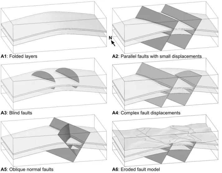
We propose a suite of relatively simple models numbered A2 to A6 that are all derived from model A1, a simple cylindrical anticline composed of three gently folded horizons where each layer has a constant thickness (Fig. 5). In model A2, two regional normal faults affect the anticline (Fig.5). These faults are planar, parallel one to another, cut the whole volume of interest, and have dips close to 60 degrees toward the west. Moreover, they have a constant total slip, corresponding to parallel horizon cutoff lines. In model A3, the regional faults are restricted to an ellipsoid shape and terminate in the model (Fig.5). These faults do not compartmentalize the domain and fault slips vary from a maximum near fault centers to zero at fault tips. In model A4, one fault is regional while the eastern fault dies out to the north (Fig. 5). Fault displacements increase to the south. As a result, horizon cutoff lines intersect with a small angle. The faults of model A5 intersect along a branch line, resulting in a Y configuration (Fig.5). Fault slips are regular and the model can be restored to model A1 by rigid block motion. However, the slip on the west fault is close to the thickness of the top layer, which generates thin features in the Allan diagram. Model
Figure 5: Suite of benchmark models derived from a simple same fold model (dimensions 16km × 9.3km × 5km).
A6 is obtained by cutting model A4 with a topography surface. This results in numerous isolated layer parts, some of them very small when compared to the model dimensions (Fig.5).
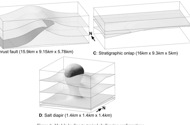
The three other models illustrate challenges arising in other contexts. Model B corresponds to a compressive fault-propagation fold (Fig. 6). In the lower part, the fault has a low dip and branches onto a horizontal d´ecollement level. The thrust dip changes to a medium angle (ramp) in the upper part and stops in the upper layer in which the shortening is accommodated by internal layer deformation. Model C is built from the folded basal horizon of model A1 overlaid by onlapping horizontal layers deposited at a low angle (Fig. 6). The diapiric dome of model D intrudes and cuts three subhorizontal layers. Except in the intrusion influence area, the horizons are only slightly deformed (Fig. 6). Dimensions for model B and C are similar to the ones for model A.
6. Results
The code implementing the measures was written in C++. From a correctly defined and sealed geological model, we compute the measures proposed in Sect.4. All these measures are computed
Figure 6: Models leading to typical challenging configurations.
for the elements that are inside the model and exclude the elements defining the volume of interest.
6.1. Global measures
The first measure, total number of elements in the model (Eq. 2), gives a first classification of the models, in increasing order: A1, C, D, B, A2, A3, A4, A5, A6 (Table 1). This classification reflects the number of discontinuities affecting the models and their connectivity. Three groups of models can be distinguished: the ones with one or no discontinuity (A1, B, C, and D), the ones with two discontinuities (A2, A3, and A4) and the ones with two or three connected discontinuities (A6 and A5). Because elements defining the volume of interest are not taken into account, this simple measure differentiates faults that terminate in the model from regional faults that cut the whole model, and A3 is considered more complex than A2.
To compute the second measure (Eq. 3) we choose a characteristic size h of 100m and an angle α at 20 degrees (Table 2). They might be seen as the desired mesh size and acceptable minimal angle for a volumetric mesh of the model. The obtained classification A1, C, B, A2, D, A4, A3, A5 and A6 is slightly different from the first one but end members remain the same: A1 is extremely simple and A6 and A5 are the most complex. The increased complexity of D is due to the fact that the dimensions of this model are significantly smaller, and its bottom region is almost completely is thinner than h. Model A3 is the third most complex model because faults ending in the model yield cutoff lines that intersect at angles inferior to 10 degrees.
The third measure (Eq. 4, Table3) gives a third classification: A1, D, B, C, A2, A4, A3, A5, A6 that is similar to the previous ones. Its meaning is however different since it identifies complexity sources due to element scale variations in the models.
A1 A2 A3 A4 A5 A6 B C D Regions 4 12 4 8 12 14 5 4 5 Surfaces 3 23 16 23 31 42 8 4 6 Lines 0 13 24 22 30 44 4 1 2 Corners 0 0 12 6 10 15 0 0 0 Total 7 48 56 59 83 115 17 9 13
Table 1: Number of elements inside the models (Eq. 2).
A1 A2 A3 A4 A5 A6 B C D
Regions 0.13 0.59 0.22 0.34 1.19 6.58 0.35 0.55 2.97
Surfaces 0.03 3.21 12.01 7.41 9.30 12.58 0.25 0.00 1.20
Lines 0.00 0.01 0.56 0.10 4.01 2.92 0.00 0.00 1.62
Total 0.16 3.81 12.79 7.85 14.50 22.07 0.60 0.55 5.79
Table 2: One geometrical complexity of elements type per type (Eq. 3).
A1 A2 A3 A4 A5 A6 B C D
Regions 0.74 0.76 0.74 0.84 1.08 1.67 0.57 0.94 0.54 Surfaces 0.00 0.93 1.97 1.41 1.74 1.62 0.79 0.71 0.56
Lines 0.01 0.63 0.67 0.82 1.06 0.00 0.13
Total 0.74 1.71 3.35 2.92 3.64 4.35 1.37 1.65 1.23
All elements A1 A2 A3 A4 A5 A6 B C D 100 Q10 1 1 1 1 1 2 3 1 3 Q50 5 5 5 5 5 7 5 5 5 Q90 7 11 10 11 11 12 7 8 6 Max 7 15 15 16 30 22 8 8 9 Mean 4.300 5.950 5.210 5.630 5.510 6.710 4.290 4.040 4.060 Coeff.Var. 0.547 0.630 0.658 0.665 0.775 0.696 0.390 0.593 0.390 1000 Q10 1 1 1 1 1 1 1 1 1 Q50 1 3 1 3 3 3 3 1 3 Q90 5 7 5 7 6 7 5 5 5 Max 7 15 13 14 22 19 6 8 6 Mean 2.500 3.137 2.710 2.960 2.950 3.170 2.630 2.360 2.569 Coeff.Var. 0.751 0.814 0.808 0.804 0.858 0.871 0.523 0.813 0.581 10000 Q10 1 1 1 1 1 1 1 1 1 Q50 1 1 1 1 1 1 1 1 1 Q90 3 3 3 3 3 3 3 3 3 Max 5 11 11 12 19 15 6 6 6 Mean 1.688 1.910 1.746 1.850 1.840 1.920 1.770 1.570 1.760 Coeff.Var. 0.728 0.788 0.755 0.778 0.795 0.827 0.609 0.721 0.676 Table 4: Statistics of the number of elements per cell for the models.
6.2. Local measures
The local measures have been made at three different resolutions using respectively 100; 1000; 10000 cells. Considering only the number of cells permits to compare models independently of their dimensions. For models A, B and C average cell sizes are 1980m, 919m, and 427m respectively; model D is smaller and the corresponding sizes are 265m, 123m, and 57m.
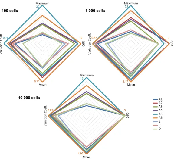
The statistics of the number of elements per cell are given in Table 4. The mean, maximum, coefficient of variation, and the 90th percentile are drawn in a radar chart (Fig. 7). For a given statistic, the relative classification of the models at the considered resolutions varies slightly. How-ever the distinction between the simplest models that have none or one discontinuity (A1, B, C, and D) and the more complex ones that contains at least two discontinuities (A2, A3, A4, A5, and A6) is clear for almost all statistics and resolutions. An obvious and expected observation is that when resolution increases, local complexity decreases and differences between models de-crease. The mean is strongly impacted by this decrease, for example the mean in A5 diminishes from 5.51 (100 cells) to 1.84 (10000 cells) that is a loss of 66.6%, the maximum only decreasing from 30 to 19 (36.6%). The maximum characterizes the most complex zone of the model, i.e., the cell that contains an element that is on the boundary of the greatest number of elements (typically a corner or a contact line). According to this criterion, the obtained classification with 10000 cells is: B, D, A1, C, A3, A2, A4, A6, A5. The 90th percentile is the same for all the models at the
smallest resolution (the value 3 corresponds to a cell intersecting one surface and two regions), but it may permit to classify the models at lower resolutions. The coefficient of variation evaluates the dispersion of the measures and can also be used as a complexity measure.
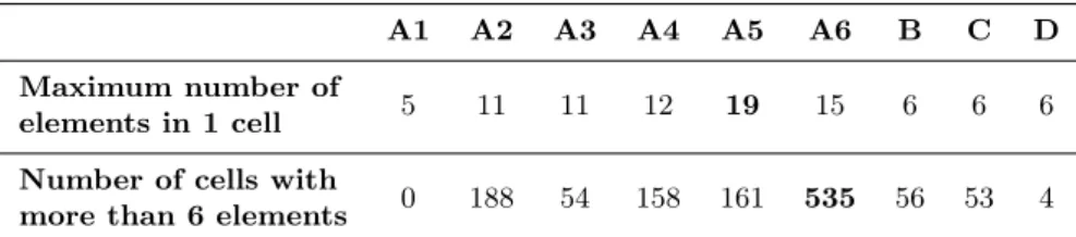
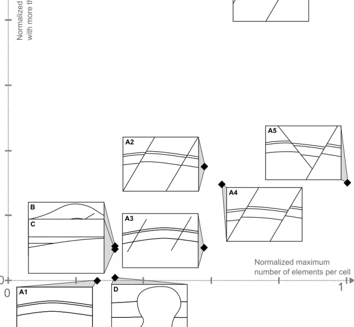
One of the main advantages of these local measures is the possibility to understand the spatial organization of the complexity and estimate the extension of the zones where a given geomodeling method will fail from the cells in which the total number of elements is above a given number. These cells are the ones closest to the thin features of the models, but also to their corners and contact lines (Fig.9). Combining the number of cells that contains more than 6 model elements
A1 A2 A3 A4 A5 A6 B C D Maximum number of
5 11 11 12 19 15 6 6 6
elements in 1 cell Number of cells with
0 188 54 158 161 535 56 53 4 more than 6 elements
Table 5: Chosen statistics evaluating the local model complexity (resolution: 10000 cells), see also Figure8.
and the maximum number of elements in all cells permits to establish a visual classification of the models (Fig. 8and Table 5).
7. Discussion
In this paper, we proposed to use general measures to evaluate the complexity of structural models defined by a set of triangulated surfaces. The metrics derived from these measures and the proposed benchmark models are important tools to quantify our perception of structural model complexity. We believe these measures could be useful for five purposes: (i) to help understand the complexity induced by each element of a model; (ii) to compare geological models (models of the same zone at different resolutions, or models of two different zones); (iii) to improve the objective comparison of geomodeling algorithms and computer codes (an objective comparison of algorithms requires an objective comparison of the models on which they succeed or fail); (iv) as an indicator of the required modeling effort to build or process these models; (v) to understand and sample the uncertainty about a structural model. In mathematical terms, complexity directly relates to the number of non-redundant parameters in a model. In assessing uncertainty, the notion of complexity is therefore important because it impacts the structure of the space of uncertainty and how model calibration methods will behave (Christie,2011;Lindsay et al.,2013b).
There are many interesting perspectives for this work. The measures could be used to determine the necessary resolution to to create a volumetric mesh conformal to the boundary representation
(Quadros et al., 2004). They also could be combined and weighted to evaluate the complexity
of a given modeling task. This requires (i) to perfectly understand the involved methods and algorithms, (ii) to consider the representation of the model (mesh size and quality), and (iii) to realize sensitivity analysis. For example, a criterion determining if a given meshing method will permit to reach the desired element quality while respecting a maximum number of cells could be developed. Additional applications would permit to refine our observations and to confirm the influence of the identified configurations on structural complexity. In particular, these applications could be made on several real or synthetic models built at different levels of details to evaluate the impact of complexity on a given model purpose. Type-specific complexity measures could also pro-vide supplementary information. For example, for fault surfaces, the number of intersected layers, displacement distribution, fault-horizon angles, induced layer contacts are crucial in geomodeling. To compute the complexity of a fault network, the connections between different faults and the variations of orientations are important. For the layers, the number of fault blocks, deformation intensity, and thickness variations could be considered. Geometry measure computations (Eq. 3) could also be performed in the neighborhoods of points, provided that adequate averaging strategies in each cell are developed. This would permit to locally characterize the complexity independently of the model representation (its mesh quality and resolution). We could also consider other cells
Figure 9: Cells containing more than six elements cover complex areas that are all localized near discontinuities (see Table5for details).
like voxels or spheres to compute these local measures.
Acknowledgments
The authors are grateful to the academic and industrial sponsors of the Gocad Consortium (www.gocad.org) managed by ASGA, for funding this work. The benchmarks models were built using SKUA-GOCAD, a geomodeling software provided by Paradigm Geophysical. The authors wish to thank Vincent Nivoliers and Bruno L´evy for their implementations of the Restricted Voronoi Diagram and of the Centroidal Voronoi Diagram.
References
Andrle, R., Apr. 1996. Complexity and scale in geomorphology: Statistical self-similarity vs. characteristic scales. Mathematical Geology 28 (3), 275–293.
Bourbiaux, B., Basquet, R., Cacas, M.-C., Daniel, J.-M., Sarda, S., 2002. An integrated workflow to account for multi-scale fractures in reservoir simulation models: Implementation and benefits. In: 10th Abu Dhabi International Petroleum Exhibition and Conference. Abu Dhabi, U.A.E., paper SPE 78489.
Calcagno, P., Chil`es, J.-P., Courrioux, G., Guillen, A., Dec. 2008. Geological modelling from field data and geological knowledge: Part I. Modelling method coupling 3D potential-field interpolation and geological rules. Physics of the Earth and Planetary Interiors 171 (1-4), 147–157.
Caumon, G., Lepage, F., Sword, C. H., Mallet, J.-L., 2004. Building and editing a sealed geological model. Mathe-matical Geology 36 (4), 405–424.
Caumon, G., Mallet, J.-L., 2006. 3D stratigraphic models: Representation and stochastic modelling. In: Proc. Int. Assoc. for Mathematical Geology - XIth International Congress. 4p.
Caumon, G., Collon-Drouaillet, P., Le Carlier de Veslud, C., Sausse, J., Viseur, S., 2009. Surface-based 3D modeling of geological structures. Mathematical Geosciences 41 (9), 927–945.
Caumon, G., Gray, G. G., Antoine, C., Titeux, M.-O., 2013. 3D implicit stratigraphic model building from remote sensing data on tetrahedral meshes: Theory and application to a regional model of La Popa basin, NE Mexico. IEEE Transactions on Geoscience and Remote Sensing 51 (3), 1613 – 1621.
Chiaraluce, L., 2012. Unravelling the complexity of Apenninic extensional fault systems: A review of the 2009 L’Aquila earthquake (Central Apennines, Italy). Journal of Structural Geology 42 (0), 2–18.
Christie, M., 2011. Uncertainty quantification and oil reservoir modelling. In: Simplicity, Complexity and Modelling. John Wiley & Sons, Ltd, pp. 147–172.
Dromgoole, P., Speers, R., 1997. Geoscore: A method for quantifying uncertainty in field reserve estimates. Petroleum Geoscience 3 (1), 1–12.
Du, Q., Faber, V., Gunzburger, M., 1999. Centroidal Voronoi Tesselations: Applications and algorithms. SIAM Review 41 (4), 637–676.
Durand-Riard, P., Caumon, G., Muron, P., 2010. Balanced restoration of geological volumes with relaxed meshing constraints. Computers and Geosciences 36 (4), 441–452.
Farmer, C. L., 2005. Geological modelling and reservoir simulation. In: Iske, A., Randen, T. (Eds.), Mathematical Methods and Modelling in Hydrocarbon Exploration and Production. Vol. 7. Springer-Verlag, Berlin/Heidelberg, pp. 119–212.
Frank, T., Tertois, A.-L., Mallet, J.-L., 2007. 3D-reconstruction of complex geological interfaces from irregularly distributed and noisy point data. Computers and Geosciences 33 (7), 932–943.
Gell-Mann, M., 1995. What is complexity. Complexity 1 (1), 16–19.
Groshong, R. H., 2006. 3D structural geology: A practical guide to surface and subsurface map interpretation, 2nd Edition. Springer-Verlag, Berlin.
Hillier, M. J., Schetselaar, E. M., de Kemp, E. A., Perron, G., Jul. 2014. Three-dimensional modelling of geological surfaces using generalized interpolation with radial basis functions. Mathematical Geosciences.
Jolley, S. J., Barr, D., Walsh, J. J., Knipe, R. J., 2007. Structurally complex reservoirs: An introduction. Geological Society, London, Special Publications 292 (1), 1–24.
Kruhl, J. H., Jan. 2013. Fractal-geometry techniques in the quantification of complex rock structures: A special view on scaling regimes, inhomogeneity and anisotropy. Journal of Structural Geology 46 (0), 2–21.
Lindsay, M., Jessell, M., Ailleres, L., Perrouty, S., de Kemp, E., Betts, P., 2013. Geodiversity: Exploration of 3D geological model space. Tectonophysics 594, 27–37.
Lindsay, M. D., Perrouty, S., Jessell, M. W., Ailleres, L., Nov. 2013b. Making the link between geological and geophysical uncertainty: Geodiversity in the Ashanti Greenstone Belt. Geophysical Journal International 195 (2), 903–922.
L´evy, B., Bonneel, N., 2013. Variational anisotropic surface meshing with Voronoi parallel linear enumeration. In: Jiao, X., Weill, J.-C. (Eds.), Proceedings of the 21st International Meshing Roundtable. Springer Berlin Heidelberg, Berlin, Heidelberg, pp. 349–366.
Mallet, J.-L., 2002. Geomodeling. Applied Geostatistics. Oxford University Press, New York, NY, 624 p. Manson, S. M., 2001. Simplifying complexity: A review of complexity theory. Geoforum 32 (3), 405 – 414.
Manzocchi, T., Sep. 2002. The connectivity of two-dimensional networks of spatially correlated fractures. Water Resources Research 38 (9), 1–1–1–20.
Matthai, S. K., Geiger, S., Roberts, S. G., Paluszny, A., Belayneh, M., Burri, A., Mezentsev, A., Lu, H., Coumou, D., Driesner, T., 2007. Numerical simulation of multi-phase fluid flow in structurally complex reservoirs. Geological Society, London, Special Publications 292 (1), 405–429.
Mustapha, H., Mustapha, K., 2007. A new approach to simulating flow in discrete fracture networks with an optimized mesh. SIAM J. Sci. Comput. 29 (4), 1439–1459.
Pellerin, J., L´evy, B., Caumon, G., Botella, A., 2014. Automatic surface remeshing of 3D structural models at specified resolution: A method based on Voronoi diagrams. Computers & Geosciences 62 (0), 103 – 116.
Quadros, W. R., Owen, S. J., Brewer, M. L., Shimada, K., 2004. Finite element mesh sizing for surfaces using skeleton. In: Proc. 13th International Meshing Roundtable. p. 389–400.
Ravaut, C., Operto, S., Improta, L., Virieux, J., Herrero, A., Dell’Aversana, P., 2004. Multiscale imaging of complex structures from multifold wide-aperture seismic data by frequency-domain full-waveform tomography: Application to a thrust belt. Geophysical Journal International 159 (3), 1032–1056.
Rossignac, J., 2005. Shape complexity. The visual computer 21 (12), 985–996.
Sassi, W., Colletta, B., Bal´e, P., Paquereau, T., Nov. 1993. Modelling of structural complexity in sedimentary basins: The role of pre-existing faults in thrust tectonics. The origin of sedimentary basins: Inferences from quantitative modelling and basin analysis 226 (1–4), 97–112.
Sukumar, S. R., Page, D. L., Koschan, A. F., Abidi, M. A., 2008. Towards understanding what makes 3D objects appear simple or complex. In: Computer Vision and Pattern Recognition Workshops, 2008. CVPRW’08. IEEE Computer Society Conference on. IEEE, pp. 1–8.
Tavassoli, Z., Carter, J. N., King, P. R., 2005. An analysis of history matching errors. Computational Geosciences 9 (2-3), 99–123.
Trubetskoy, K., Galchenko, Y., Sabyanin, G., Nov. 2012. Evaluation methodology for structural complexity of ore deposits as development targets. Journal of Mining Science 48 (6), 1006–1015.
White, D. R., Saigal, S., Owen, S. J., 2005. Meshing complexity: Predicting meshing difficulty for single part CAD models. Engineering with Computers 21 (1), 76–90.