HAL Id: hal-00305091
https://hal.archives-ouvertes.fr/hal-00305091
Submitted on 6 Sep 2007
HAL is a multi-disciplinary open access
archive for the deposit and dissemination of
sci-entific research documents, whether they are
pub-lished or not. The documents may come from
teaching and research institutions in France or
abroad, or from public or private research centers.
L’archive ouverte pluridisciplinaire HAL, est
destinée au dépôt et à la diffusion de documents
scientifiques de niveau recherche, publiés ou non,
émanant des établissements d’enseignement et de
recherche français ou étrangers, des laboratoires
publics ou privés.
Modelling the spatial variability of snow water
equivalent at the catchment scale
T. Skaugen
To cite this version:
T. Skaugen. Modelling the spatial variability of snow water equivalent at the catchment scale.
Hydrol-ogy and Earth System Sciences Discussions, European Geosciences Union, 2007, 11 (5), pp.1543-1550.
�hal-00305091�
www.hydrol-earth-syst-sci.net/11/1543/2007/ © Author(s) 2007. This work is licensed under a Creative Commons License.
Earth System
Sciences
Modelling the spatial variability of snow water equivalent at the
catchment scale
T. Skaugen
Norwegian Water Resources and Energy Directorate, P.O. Box 5091, Maj, 0301, Oslo, Norway Department of Geosciences, University of Oslo, P.O. Box 1047, Blindern, Oslo, Norway Received: 16 May 2007 – Published in Hydrol. Earth Syst. Sci. Discuss.: 8 June 2007 Revised: 29 August 2007 – Accepted: 5 September 2007 – Published: 6 September 2007
Abstract. The spatial distribution of snow water equiva-lent (SWE) is modelled as a two parameter gamma distri-bution. The parameters of the distribution are dynamical in that they are functions of the number of accumulation and melting events and the temporal correlation of accumula-tion and melting events. The estimated spatial variability is compared to snow course observations from the alpine catch-ments Norefjell and Aursunden in Southern Norway. A fixed snow course at Norefjell was measured 26 times during the snow season and showed that the spatial coefficient of varia-tion change during the snow season with a decreasing trend from the start of the accumulation period and a sharp increase in the melting period. The gamma distribution with dynami-cal parameters reproduced the observed spatial statistidynami-cal fea-tures of SWE well both at Norefjell and Aursunden. Also the shape of simulated spatial distribution of SWE agreed well with the observed at Norefjell. The temporal correla-tion tends to be positive for both accumulacorrela-tion and melting events. However, at the start of melting, a better fit between modelled and observed spatial standard deviation of SWE is obtained by using negative correlation between SWE and melt.
1 Introduction
A major cause of severe flooding in Norway is the combina-tion of intense snowmelt and heavy precipitacombina-tion. In order to forecast these events, we need reliable forecasts of precipita-tion and temperature and a good estimate of the snow reser-voir and its coverage in the catchment at the time of the fore-cast. The dynamics of runoff due to snowmelt, and thus the water balance in the melting season, is very dependent on the evolution of snow free areas, which again is closely linked Correspondence to: T. Skaugen
to the spatial distribution of snow water equivalent (SWE) (Pomeroy et al., 2004; Luce et al., 1998; Buttle and McDon-nel, 1987). The shape of the distribution is important in order to describe the development of snow free areas in spring. A skewed distribution with high frequencies of small values of SWE would produce more snow free areas in response to uniformly distributed melt than would a more normal distri-bution of SWE where the highest frequencies are found for higher values of SWE. Increased production of snow free ar-eas for skewed distributions will occur in cases where the spatial distribution of daily melt is inversely correlated to the distribution of SWE as reported by Faria et al. (2000).
Positively skewed distributions like the exponential (Gao and Sorooshian, 1994) and gamma (Onof et al., 1998; Mackay et al., 2001) have often been favoured for describ-ing the spatial distribution of daily precipitation. As the accumulated SWE is the sum of such positively skewed and correlated variables, one would expect the distribution of SWE to be subject to the central limit theorem (Feller, 1971, p. 258) and being less skewed than the distribution of the individual snowfall events. The normal distribution has often been found to be a good model for describing SWE at its seasonal maximum (Marchand and Killingtveit, 1999, 2002; Alfnes et al., 2004), which indicates that the spatial distribution of SWE evolves from a rather skewed distribution at the beginning of the snow season towards a less skewed, (even normal) distribution at its seasonal maxi-mum. The Swedish HBV model (Bergstrøm, 1992; Sælthun, 1996) is used operationally for flood forecasting at the Nor-wegian Water Resources and Energy Directorate (NVE) and has been supplemented with a snow routine developed for use in Norway which accounts for the development of the snow reservoir and the snow coverage at different altitude levels (Killingtveit and Sælthun, 1995). This routine is devel-oped under the assumptions that precipitation as snow is log-normally distributed in space with a fixed coefficient of vari-ation. Donald et al. (1995) presented a snow accumulation
1544 T. Skaugen: Spat-var-SWE model where, once the snow coverage was 100%, the
spa-tial variability of SWE remained constant. These static ways of representing the spatial distribution of SWE are thus in conflict with the central limit theorem, reported observations (Alfnes et al., 2004; Pomeroy et al., 2004) and observations presented in this paper.
Skaugen et al. (2004) put forward a formulation for the spatial distribution of snow, using the fact that when individ-ual snowfall events are gamma distributed, the distribution of accumulated snowfall events is also gamma distributed with parameters derived from the parameterisation of indi-vidual snowfall events and the number of accumulations. This model is constrained by assumptions of independence in time, but takes into account that the statistical features of the spatial distribution of SWE change during the season, as demonstrated from observations. The dynamical aspect of the shape of the spatial distribution of SWE is a feature that has to be included in the modelling of SWE in order to sim-ulate realistic snow distributions
Observed differences for spatial distributions of SWE at the peak of accumulations has been addressed to landscape and meteorological features such as vegetation type, to-pography and wind (Erickson et al., 2005; Bruland et al., 2004; Alfnes et al., 2004; Marchand and Killingtveit, 2004; Erxleben et al., 2002; Shook and Gray, 1997). According to Liston (2004), three mechanisms effective on different spa-tial scales influence the snowdepth. Snow-canopy interac-tions in forested regions are important at one to hundreds of meters, snow redistribution by wind on tens to hundreds of metres and orographic influences of precipitation being ac-tive on one to a few kilometres. The latter spatial scale is the relevant scale for this study and for describing the spatial dis-tribution of SWE in lumped hydrological models such as the operational HBV model. It is the objective of this study to demonstrate that the spatial distribution of SWE can be ad-equately modelled as the summation of correlated (in time) daily precipitation (snowfall) fields. The sources of variabil-ity at smaller scales, like snow-canopy interactions and wind drift are, in this study, not taken into account.
We want to develop dynamical expressions for the spatial variability of SWE both for the accumulation and the melting season. We further want to use this information to assign an-alytical expressions for the spatial distribution of SWE. The proposed methodology will be validated against time series of the spatial distribution of SWE measured at alpine loca-tions in Southern-Norway.
The next section presents the derivation of expressions for the spatial moments of SWE, where temporal correlation is taken into account. The moments are then used for esti-mating the parameters of the spatial distribution of SWE. The third section presents a snow monitoring campaign spe-cially designed for studying the spatial distribution of SWE throughout the snow season. In the fourth section the mod-elled moments and distributions are tested against observed
data and discussed, whereas conclusions are found in the fi-nal section.
2 Modelling accumulation and melt of snow as sums of correlated gamma distributed stochastic fields When modelling the spatial distribution of SWE, we have to take into account the history of accumulation and melting events up to the time of interest. In Skaugen et al. (2004) this was carried out by modelling the spatial distribution of SWE as sums of independent, identically distributed stochas-tic fields of the two parameter gamma distribution. Here, the spatial distribution of SWE is also modelled within the framework of the two parameter gamma distribution, but, through a simple procedure, the effect of temporal correla-tion is introduced.
Let us assume that every snow fall event can be described as a collection of gamma distributed stochastic unit fields of snowfall, y. The stochastic unit fields of snowfall y is distributed in space according to a two-parameter gamma
distribution, y=G(ν0, α0), with probability density function
(PDF): fα0,ν0(y) = 1 Ŵ(ν0) αν0 0 y ν0−1e−α0y α 0, ν0, y > 0 (1)
where α0 and ν0 are parameters. The mean equals
E(y)=ν0/α0 and the variance equals Var(y)=ν0/α02. The
stochastic unit fields are hereafter, for practical purposes, de-noted units. The choice of distribution is motivated partly from studies reporting the gamma distribution as a suit-able choice of spatial distribution for precipitation (Onof et al., 1998; Mackay et al., 2001) and SWE (Kutchment and Gelfan, 1996) and partly because of the practical mathemat-ical features of the gamma distribution and the flexibility needed for representing the observed changes in the shape of the spatial distribution during the snow season. We want to describe the moments of the accumulated snow reservoir z(t ), accumulated at time t, z(t )=
n(t )P
i=1
yi, where n is the
num-ber of units y accumulated up to the time t. The mean of z(t )is E(z(t )) = n X i=1 E(yi) = n ν0 α0 , (2)
whereas for the variance of z(t ) we have to take into account the temporal correlation of y and we have to consider the covariance matrix of z(t ) (see Haan, 1977, p. 56):
Var(z(t )) = n(t ) X i=1 Var(yi) + 2 X i<j Cov(yi, yj) (3)
In the following, we assume that the covariance between the units can be described as a constant fraction c of the variance,
Var(y), of the individual y’s, Cov(yi, yj)=cVar(y)=cν0
α20.
The variance of z(t ) becomes:
Var(z(t )) = nν0 α02 +n(n − 1)cν0 α02 =nν0 α02(1 + (n − 1)c) (4)
We note that c=Cov(yVar(y)i,yj)is the correlation coefficient, given
that yi and yj are identically distributed. This correlation
function should be a decreasing function with time, but is here represented with its temporal average over all the n units.
We want the spatial distribution of accumulated snow z(t ) at all times to be simple mathematically tractable distribu-tion funcdistribu-tion, with which we easily can simulate and per-form other exploratory analyses. We thus state that z(t ) is
distributed as a gamma distribution with parameters nνnand
αn. In order to formulate the moments of the sum of the
gamma distributed variables in this manner, the n elements of the sum have to be independent, and identically gamma
distributed variables with parameters νnand αn (see Feller,
1971, p. 47). Let us denote these independent variables as
Yi. The mean and variance of z(t ) modelled as a sum of
in-dependent variables, Y are: E(z(t )) = nνn αn (5) and Var(z(t )) = nνn α2 n (6) From the mean and variance of z(t ) modelled as a sum of
dependent variables, y, we can determine expressions for νn
and αnby the mean and variance of z(t ) modelled as a sum of
independent variables, Y . From the equating of Eqs. (2) and
(5), nν0
α0=n
νn
αn and Eqs. (4) and (6), n
ν0
α02(1+(n−1)c)=n
νn
α2
n
we can solve for νnand αnand get:
αn= α0 1 + (n − 1)c (7) and νn= ν0 1 + (n − 1)c (8)
We note that the ratios νn
αn and
ν0
α0 are equal, which mean that
the mean of the process is unaffected by the correlation.
2.1 Adding correlated variables to a sum of independent
variables
Let us say at time t′an additional snowfall of u units of y,
have fallen on z(t ) giving us the snow reservoir z(t′),
z(t′) = Y1+Y2+.. + Yn+y1+y2+.. + yu (9) The mean can be estimated straightforwardly as the sum of the individual means:
E(z(t′)) = n X i=1 E(Yi) + u X i=1 E(yi) = n νn αn +uν0 α0 (10)
For the variance of z(t′) we must again consider the
covari-ance matrix of Var(z(t′)) and V ar(z(t′)) is the sum of all the
elements of the covariance matrix. Given that the Y ’s are un-correlated, the covariance elements describing the covariance between the Y ’s are zero and we get the following expression
for the variance z(t′):
Var(z(t′)) = n X j =1 Var(Yj)+2 n X j =1 u X i=1 Cov(Yj, yi) + u X i=1 Var(yi)+2 u−1 X i=1 u X k=i+1 Cov(yi, yk) (11)
We assume also here that Cov(Y, y) can be approximated by
Cov(Y, y)=cVar(y)=cν0
α20, and Eq. (11) can be written as:
Var(z(t′)) = nνn α2 n +uν0 α02+2nuc ν0 α02 +u(u − 1)c ν0 α02 (12) From Eqs. (10) and (12), we can develop expressions for the
parameters of the distributions of z(t′) modelled as a sum of
n+u independent gamma distributed events with moments E(z(t′))=nνn+u
αn+u and Var(z(t
′))=nνn+u α2n+u: αn+u = (n + u)νn αn nνn α2 n + ν0 α2 0 (u + 2nuc + u(u − 1)c) (13) and νn+u= (n + u)(νn αn) 2 nνn α2 n + ν0 α02(u + 2nuc + u(u − 1)c) (14) 2.2 Melting events
We can, in a similar way as above, develop the moments for the accumulated SWE after a melting event. Let us say
at time t′ a melting event takes place and u units of y, are
melted from z(t ) giving us the snow reservoir z(t′),
z(t′) = Y1+Y2+.. + Yn−y1−y2−.. − yu (15) We make here the assumption that the spatial distribution of a unit melt is identical to that of a unit snowfall. It is diffi-cult to have strong assumptions on the spatial distribution of snow melt, other than that the ultimate melting event is nec-essarily identically distributed as the ultimate SWE. Essery and Pomeroy (2004) assumed a log-normal distribution of snowmelt from log-normally distributed SWE, a distribution of melt which is similar in shape to the gamma distribution. This issue is further discussed in Sect. 4.
The mean can, as above, be estimated straightforwardly as the sum of the individual means:
E(z(t′)) = n X i=1 E(Yi) − u X i=1 E(yi) =n νn αn −uν0 α0 (16)
1546 T. Skaugen: Spat-var-SWE 60˚ 64˚ 4 8 12
Oslo
.
.
Norefjell
Aursunden
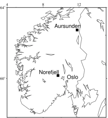
Fig. 1. Locations of snow monitoring campaigns at Norefjell and Aursunden, Southern Norway.
and we have the following expression for the variance of z(t′): Var(z(t′)) = n X j =1 Var(Yj) − 2 n X j =1 u X i=1 Cov(Yj, yi) + u X i=1 Var(yi) + 2 u−1 X i=1 u X k=i+1 Cov(yi, yk) (17)
We get negative and positive covariance contributions from the melting event. The negative contributions come from when the melting event is correlated to the snow reser-voir prior to the melting. A melting unit correlated with a melting unit gives a positive contribution. Also here we make the assumption that Cov(Y, y)can be approximated by
Cov(Y, y)=cVar(y)=cν0
α2
0
, and Eq. (17) can be written as:
Var(z(t′)) = n ν α2+u ν0 α02−2nuc ν0 α02+u(u − 1)c ν0 α02 (18) From Eqs. (16) and (18), we can develop expressions for the
parameters of the distributions of z(t′) modelled as n−u
in-dependent gamma distributed events: αn−u= (n − u)νn αn nνn α2 n + ν0 α20(u − 2nuc + u(u − 1)c) (19) and νn−u= (n − u)(νn αn) 2 nνn α2 n +ν0 α2 0 (u − 2nuc + u(u − 1)c) (20) 0 50 100 150 200 250 300 350 400 450 500 2 1 .1 1 .2 0 0 2 2 1 .1 2 .2 0 0 2 2 1 .0 1 .2 0 0 3 2 1 .0 2 .2 0 0 3 2 1 .0 3 .2 0 0 3 2 1 .0 4 .2 0 0 3 2 1 .0 5 .2 0 0 3 2 1 .0 6 .2 0 0 3 2 1 .0 7 .2 0 0 3 2 1 .0 8 .2 0 0 3 2 1 .0 9 .2 0 0 3 2 1 .1 0 .2 0 0 3 2 1 .1 1 .2 0 0 3 2 1 .1 2 .2 0 0 3 2 1 .0 1 .2 0 0 4 Time m m 0 0.1 0.2 0.3 0.4 0.5 0.6 0.7 0.8 C V
Fig. 2. Observed spatial mean (solid line), spatial standard deviation (long dashed line) and CV (short dashed line) of SWE at Norefjell.
3 Snow course data from Norefjell – Southern Norway During the EU project Envisnow, montoring of the spatial distribution of SWE during the snow season was performed
at Norefjell (60◦15′N, 9◦30′E) located in southern Norway
110 km north-east of Oslo (see Fig. 1). The motivation for the monitoring campaign was to study the possible change in features of the spatial distribution of SWE trough the snow season. The snow monitoring campaign was carried out do-ing snow surveys every second week in the accumulation sea-son and every week during the melting seasea-son. The route was fixed (by GPS) for the 2 km long snow course and snow depth was measured every 10 m. Snow density was measured twice during the snow course at locations of the mean snow depth. The snow course route is located at 1100 m a.s.l. and is above the tree line. 17 one-day campaigns between Novem-ber 2002 and June 2003, and 9 campaigns between OctoNovem-ber 2003 and February 2004 were carried out. The latter part of the monitoring period also includes the start of the accu-mulation period, whereas the former started when there were already 200 mm of SWE present.
Figure 2 shows the time series of the mean, standard devi-ation and coefficient of varidevi-ation (CV) of SWE for the snow course data. We can note that the CV (see October 2003) is relatively high at the start of the accumulation season, de-creases during the accumulation season, and rises sharply during the melting season. As the mean SWE and the stan-dard deviation both decrease during the melting season, the increasing CV implies that the rate of change (decrease) of the mean is much higher than for the standard deviation. This feature of the spatial standard deviation of SWE was also noted by Pomeroy et al. (2004), who found that the other-wise strong association between mean SWE and standard de-viation was not evident during melt. During melt, the mean SWE declined whereas the standard deviation increased or remained constant.
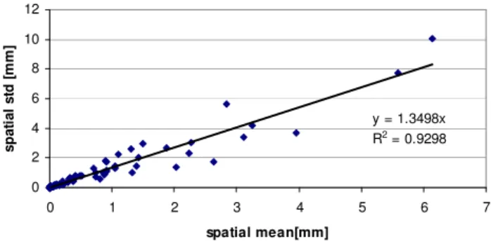
y = 1.3498x R2 = 0.9298 0 2 4 6 8 10 12 0 1 2 3 4 5 6 7 spatial mean[mm] s p a ti a l s td [ m m ]
Fig. 3. Spatial analysis of precipitation from five gauges in the Norefjell area. Spatial mean of precipitation versus the spatial stan-dard deviation. The spatial stanstan-dard deviation can be modelled as a linear function of the spatial mean.
4 Results and discussion
The dynamical parameters α and ν of the two parameter gamma distribution was calculated for each point of obser-vation of mean SWE, taking into account accumulation and melting events by using the Eqs. (13) and (14), or (19) and (20), respectively. The mean areal SWE acts as input and,
after the parameters c, α0 and ν0 have been assigned
esti-mated values, the proposed method estimates the parameters of the spatial distribution of SWE modelled as a two param-eter gamma distribution.
In order to estimate the parameters of the distribution of a
stochastic unit field of snow fall, α0and ν0, an analysis of the
spatial statistics of precipitation in the area was carried out using the daily rainfall fields measured for a year from four nearby stations (the snow course site is situated in the centre of a square defined by the four stations). The events anal-ysed where screened so that at least one station (of the four) measured zero precipitation. This strategy was chosen so we could be sure of that the spatial distributions analysed were not bounded to the left by values higher than zero, which would not be consistent with our definition of a stochastic unit field as distributed as a two parameter gamma distribu-tion. Figure 3 shows the scatter plot of observed spatial mean
and spatial standard deviation (R2=0.93), indicating a more
or less a constant spatial coefficient of variation, CV=1.35. This feature is also observed by Barancourt et al. (1992) for spatial precipitation events in France. The very high ob-served correlation between spatial mean and standard ation suggests that we can estimate the spatial standard devi-ation of the unit stochastic field to be 1.35 times the mean. Let us say that the spatial unit of snow fall has a spatial mean equal to the daily mean of positive precipitation (exclud-ing zero events) of the closest precipitation station located 18 km south of the snow course site and 367 m a.s.l. This is equivalent to the procedure used when using point observa-tion(s) to estimate the spatial mean as input in rainfall runoff models. For Norefjell this procedure gives us the estimates
0 20 40 60 80 100 120 140 2 1 .1 1 .2 0 0 2 2 1 .1 2 .2 0 0 2 2 1 .0 1 .2 0 0 3 2 1 .0 2 .2 0 0 3 2 1 .0 3 .2 0 0 3 2 1 .0 4 .2 0 0 3 2 1 .0 5 .2 0 0 3 2 1 .0 6 .2 0 0 3 2 1 .0 7 .2 0 0 3 2 1 .0 8 .2 0 0 3 2 1 .0 9 .2 0 0 3 2 1 .1 0 .2 0 0 3 2 1 .1 1 .2 0 0 3 2 1 .1 2 .2 0 0 3 2 1 .0 1 .2 0 0 4 Time s td [m m ]
Fig. 4. Observed (solid line) and estimated spatial standard devia-tion at Norefjell. Long dashed line represents estimates by the new model and short dashed line represents estimates by the snow rou-tine of the HBV-model.
of spatial mean and standard deviation as m=5.86 mm and s=7.91 mm, respectively. The parameters were estimated
trough the relations α0=m/s2and ν0=m2/s2.
It can be argued that the estimate for the spatial variability of precipitation used here for estimating the parameters of
the stochastic unit fields (α0and ν0) is too large and cannot
be representative for such a small spatial scale as that of the snow course (2 km). If such an overestimation was substan-tial, we would probably overestimate the spatial variance, as the covariance, in the accumulation phase, represents a pos-itive contribution to the spatial variance (see Eq. 3). It is possible that the correlation coefficient c (which is a tuned parameter and not estimated from data) compensates for this, and that it should, in reality, be higher.
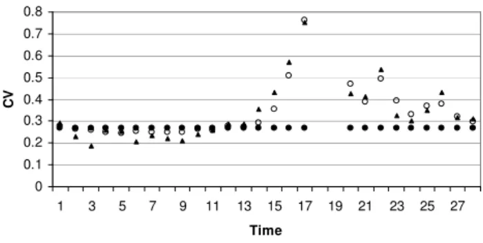
The correlation coefficient c was tuned in order to get an optimal fit of estimated spatial standard deviation of SWE. The optimality of the fit is measured by the Nash and Sut-cliffe coefficient of efficiency R2 (Nash and SutSut-cliffe, 1970). The estimated time series of standard deviation and CV of SWE is also compared to that estimated by the traditional snow routine of the HBV models which uses a lognormal distribution with a fixed CV (optimized by the R2 criterion). Figure 4 shows observed and estimated (by the proposed model and by HBV) values of the spatial standard deviation of SWE and Fig. 5 shows observed and estimated CV. The R2 value for the estimate of the spatial standard deviation was R2=0.87 for the new model, and R2=0.32 for the snow rou-tine of the HBV model. The new model is thus a considerable improvement to the lognormal distribution with a fixed CV. The observed values do indeed show that the spatial distribu-tion of SWE changes through the season, and the proposed model capture these changes well. Figure 6 shows the agree-ment between the gamma CDFs (1000 values are simulated) based on the estimated values of α and ν and the empirical CDFs from the observations for the dates 18 March 2003 and 28 May 2003, confirming that a representative model for the spatial distribution of SWE is developed.
1548 T. Skaugen: Spat-var-SWE 0 0.1 0.2 0.3 0.4 0.5 0.6 0.7 0.8 1 3 5 7 9 11 13 15 17 19 21 23 25 27 Time C V
Fig. 5. Observed (black triangles) and estimated CV at Norefjell. Open circles represent estimates by the new model and black circles represent estimates by the snow routine of the HBV-model (fixed CV value). 0 100 200 300 400 500 600 700 800 900 0 0.2 0.4 0.6 0.8 1
Fig. 6. Observed and simulated spatial CDF of SWE at near snow maximum (18 March, and late spring (28 May) at Norefjell. Solid lines are observed values (thick line at 18 March), and dashed lines are simulated (long dashed lines at 18 March).
Unfortunately no validation data from this site is avail-able. However, when the sample of SWE was split and the method was calibrated for the 2002–2003 data and validated for the 2003–2004 data, very good results were obtained with R2=0.86 for the calibration period and R2=0.90 for the val-idation period.
In this study we have assumed identical distributions of stochastic unit fields of accumulation and of melt. Observed spatial fields of snowmelt are scarce but from a research site near Trondheim in central Norway, 4 snow pillows is located
within 25 m2. For the month of April 2007 we could observe
17 daily melting events measured at the 4 snow pillows. It is, obviously, difficult to make inferences on the spatial distri-bution from four values covering such a tiny area, but Fig. 7 shows how the spatial CV decreases as the spatial mean in-creases. This behaviour of CV versus spatial mean is sim-ilar to what can be seen for the accumulation of SWE (see Fig. 2) and consistent with modelling melt as summations of temporally correlated spatial fields, of which each can well be gamma distributed. The spatial distribution of daily melt, measured on fixed time intervals is obviously non-stationary. The proposed method takes the non-stationarity of melt into
0 0.2 0.4 0.6 0.8 1 1.2 1.4 0 10 20 30 40 50 60 daily mean [mm] C V
Fig. 7. Spatial CV of daily melt versus spatial mean of melt. The data are from four snowpillows covering an area of 25 in the Trond-heim area during April 2007.
account in the way that different number of units (typically increasing in spring) give different spatial distributions of melt, thus mimicking a non-stationary process. The good agreement between simulated and observed CDF (Fig. 6), in late spring (28 May) shows that the assumption of identical distributions of the units of melt and accumulation is not crit-ical in respect to the performance of the model.
The optimal values for c in the Norefjell data was c=0.019. Using different values of c for accumulation and melting events were tried and, for this location, improve-ments of R2 were found. When using c=0.016 for accu-mulation events and c=0.01 for melt events, we obtained a R2=0.90. Studies of temporal correlation of precipitation, both for a fixed coordinate system and from a coordinate sys-tem that moves with the storm, show a rapidly declining cor-relation function which approaches zero after approximately two hours (Zawadski, 1973). As the parameter c represents a temporal average over the total number of events, it is thus not strange that the values obtained in this study are small. The effect of correlation, however, is significant, in that we would otherwise have a steadily increasing spatial variance as both summation and subtraction increases the variance (Haan, 1977).
It is also interesting to note that the correlation between melting events and SWE turns out to be positive. Pomeroy et al. (2004) found positive correlation between SWE and
melt on the catchment scale (>10 km2) and negative
corre-lation for smaller scales. Positive correcorre-lation was explained by the presence of landscape classes (shrub tundra) receiving more snow due to redistribution processes and the possibility of increased melt rate for areas with exposed shrub due to reduced albedo and enhanced aerodynamic roughness. We investigated the effects of varying the sign of the correlation coefficient c in Eq. (17) for melting and for different phases of the melting process. A negative correlation between melt and pre-melt SWE resulted in a steadily increasing standard deviation during the melting period and was thus not con-sistent with the observations. Negative correlation at the be-ginning of the melting period and positive towards the end
0 20 40 60 80 100 120 140 2 1 .1 1 .2 0 0 2 2 1 .0 1 .2 0 0 3 2 1 .0 3 .2 0 0 3 2 1 .0 5 .2 0 0 3 2 1 .0 7 .2 0 0 3 2 1 .0 9 .2 0 0 3 2 1 .1 1 .2 0 0 3 2 1 .0 1 .2 0 0 4 Time s td [m m ]
Fig. 8. Observed and estimated spatial standard deviation of SWE at Norefjell. The standard deviation is modelled with negative cor-relation at the start of the melting period, and positive towards the end of the melting period.
improved the fit between modelled and observed standard de-viation of SWE (R2=0.92) (see Fig. 8) and we note that the increase in standard deviation seen at the start of the melting season (see Fig. 8 when the mean SWE starts to decrease) is now well estimated due to negative correlation. A possible reason for an initial negative correlation can be the smaller demand of energy needed by shallow snow packs to reach an isothermal state and the maximum amount of retainable melt water in the snow pack. Melting will thus take place ear-lier for these shallow snow packs. The positive correlation is harder to explain if one does not take into account domi-nating landscape classes that favour both accumulation and increased melt rate. Such landscape classes are not present at the Norefjell snow course, where there are some 30–40 m of low-growing willow thicket (<60 cm) and otherwise no vegetation besides grass. Maybe the positive correlation be-comes appropriate only towards the end of the melting sea-son, when the entire snow pack is mature and producing melt. At this stage, SWE starts to be a limiting factor and more melt water is generated from larger snow packs simply be-cause more SWE is available for melting.
In order to investigate whether the method could be ap-plied also to other locations than Norefjell, we tested if the spatial variability of SWE could be reproduced at an alpine catchments at Aursunden in the northern part of Southern Norway (see Fig. 1). Snow course measurements was carried out at Aursunden (930 m a.s.l.) three times during April and May in 2002 (see Alfnes et al., 2004). Again, the route was fixed by GPS for the 1 km long snow course and snow depth
was measured every 10 m. The parameters α0and ν0were
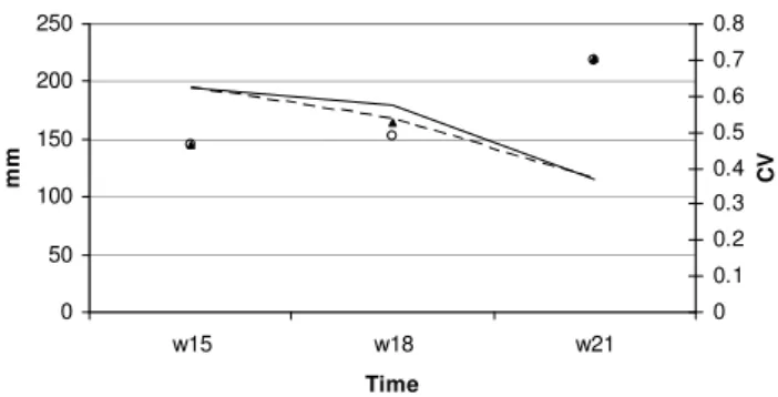
es-timated in the same manner as above from a spatial analysis of precipitation measured at five nearby gauges (spatial daily mean, m=3.31 mm, and standard deviation, s=4.15 mm). The correlation coefficient was tuned to the values of observed spatial standard deviation. Also here the best fit was ob-tained with using different values of c for melting (c=0.11) and accumulation (c=0.13) events. Figure 9 shows the good
0 50 100 150 200 250 w15 w18 w21 Time m m 0 0.1 0.2 0.3 0.4 0.5 0.6 0.7 0.8 C V
Fig. 9. Observed and estimated values of standard deviation and CV at Aursunden for the weeks 15, 18 21 in 2002. Observed val-ues of standard deviation and CV are represented by solid line and black triangles. Estimated values of standard deviation and CV are represented by long dashed line and open circles.
agreement between observed and modelled spatial standard deviation and CV. The correlation coefficient and the spatial standard deviation of precipitation take on quite different val-ues at Norefjell and Aursunden. Although the observations points are too few to make strong inferences it does seem rea-sonable that we find high temporal correlation together with relatively low spatial variability of precipitation.
5 Conclusions
A model for the spatial distribution of SWE has been put for-ward. At all times the spatial distribution of SWE can be expressed as a two parameter gamma distribution where the parameters are functions of the mean and variability of ob-served precipitation, the number of accumulation and melt-ing events and of temporal correlation.
The observed time series of SWE confirms that the spatial distribution of SWE do change trough the snow season with initially high CV, which decreases during the accumulation season and increases in the melting season. These features, as well as the shape of spatial distributions of SWE, are well reproduced by the proposed model.
The new model clearly represents the spatial distribution of SWE more realistically than the log-normal distribution with a fixed CV which is traditionally used in the HBV model in the Nordic countries. The model provides good estimates of the spatial variability of SWE at two alpine locations in Southern Norway.
Analysis of the correlations between pre melt SWE and melt suggests that correlation is negative in the early stages of the melting process and positive at later stages. Positive correlation between SWE and melt at the end of the melting proved, within the model framework, to be necessary in order to model the decrease in spatial variability observed in the snow course data.
1550 T. Skaugen: Spat-var-SWE
Acknowledgements. The efforts of my colleagues E. Alfnes,
L. Andersen, H. C. Udnæs, L. E. Petterson and S. Beldring for collecting the validation data are gratefully acknowledged. Also the comments of the two anonymous referees and the editor are highly appreciated.
Edited by: A. Gelfan
References
Alfnes, E., Andreassen, L. M., Engeset, R. V., Skaugen, T., and Udnæs, H.-C.: Temporal variability in snow distribution, Ann. Glaciol., 38, 101–105, 2004.
Barancourt, C., Creutin, J. D., and Rivoirard, J.: A method for delin-eating and estimating rainfall fields, Water Resour. Res., 28(4), 1133–1144, 1992.
Bergstr¨om, S.: The HBV model – its structure and applications, SMHI Hydrology, RH no.4, Norrk¨oping, 35 pp., 1992.
Bruland, O., Liston, G. E., Vonk, J., Sand, K., and Killingtveit, ˚
A.: Modelling the snow distribution at two high artic sites at Svalbard, Norway, and at an alpine site in central Norway, Nord. Hydrol., 35(3), 191–208, 2004.
Buttle, J. M. and McDonnel, J. J.: Modelling the areal depletion of snowcover in a forested catchment, J. Hydrol., 90, 43–60, 1987. Donald, J. R., Soulis, E. D., Kouwen, N., and Pietroniro, A.: A land cover-based snow cover representation for distributed hydrologic models, Water Resour. Res., 31(4), 995–1009, 1995.
Erickson, T. A., Williams, M. W., and Winstral, A.: Persistence of topographic controls on the spatial distribution of snow in rugged mountain terrain, Colorado, United States, Water Resour. Res., 41, W04014, doi:10.1029/2003WR002973, 2005.
Essery, R. and Pomeroy, J.: Implications of spatial distributions of snow mass and melt rate for snow-cover depletion: theoretical considerations, Ann. Glaciol., 38, 261–265, 2004.
Erxleben, J., Elder, K., and Davis, R.: Comparison of spatial in-terpolation methods for estimating snow distribution in the Col-orado Rocky Mountains, Hydrol. Processes, 16, 3627–3649, 2002.
Faria, D. A., Pomeroy, J., and Essery, R.: Effect of covariance be-tween ablation and snow water equivalent on depletion of snow-covered in a forest, Hydrol. Earth Syst. Sci., 14, 2683–2695, 2000,
http://www.hydrol-earth-syst-sci.net/14/2683/2000/.
Feller, W.: An introduction to probability theory and its applica-tions, John Wiley, New York, pp. 669, 1971.
Gao, X. and Sorooshian, S.: A stochastic precipitation disaggrega-tion scheme for GCM applicadisaggrega-tions, J. Climate, 7(2), 238–247, 1994.
Haan, C. T.: Statistical methods in hydrology, The Iowa State Uni-versity Press, Ames, Iowa, 378 pp., 1977.
Killingtveit, ˚A. and Sælthun, N.-R.: Hydrology, vol. 7 in Hy-dropower development, NIT, Trondheim, Norway, 1995. Kutchment, L. S. and Gelfan, A. N.: The determination of the
snowmelt rate and the meltwater outflow from a snowpack for modelling river runoff generation, J. Hydrol., 179, 23–36, 1996. Liston, G. E.: Representing subgrid snow cover heterogeneities in regional and global models, J. Climate, 17, 1381–1397, 2004. Luce, C. H., Tarboton, D. G., and Cooley, K. R.: The influence
of the spatial distribution of snow on basin-averaged snowmelt, Hydrol. Processes, 12, 1671–1683, 1998.
Mackay, N. G., Chandler, R. E., Onof, C., and Wheater, H. S.: Dis-aggregation of spatial rainfall fields for hydrological modelling, Hydrol. Earth Syst. Sci., 5, 165–173, 2001,
http://www.hydrol-earth-syst-sci.net/5/165/2001/.
Marchand, W.-D. and Killingtveit, ˚A.: Statistical probability distri-bution of snow on sub-grid cell level, Nordic Hydrological Pro-gramme, NHP Report No. 47, pp 461–471, 2002.
Marchand, W.-D. and Killingtveit, ˚A.: Statistical properties of snow cover in mountainous catchments in Norway, Northern Research Basins, Twelfth International symposium and Workshop, Reyk-javik, Iceland, pp. 227–239, 1999.
Marchand, W.-D. and Killingtveit, ˚A.: Statistical properties of spa-tial snow cover in mountainous catchments in Norway, Nord. Hy-drol., 35(2), 101–117, 2004.
Nash, J. E. and Sutcliffe, J. V.: River flow forecasting through con-ceptual models: Part I – A discussion of principles, J. Hydrol., 10, 282–290, 1970.
Onof, C., Mackay, N. G., Oh, L., and Weather, H. S.: An improved rainfall disaggregation technique for GCMs, J. Geophys. Res., 103(D16), 19 577–19 586, 1998.
Pomeroy, J., Essery, R., and Toth, B.: Implications of spatial dis-tributions of snow mass and melt rate for snow-cover depletion: observations in a subarctic mountain catchment, Ann. Glaciol., 38, 195–201, 2004.
Shook, K. and Gray, D. M.: Synthesizing shallow seasonal snow covers, Water Resour. Res., 33(3), 419–426, 1997.
Skaugen, T., Alfnes, E., Langsholt, E., and Udnæs, H.-C.: Time variant snow distribution for use in hydrological models, Ann. Glaciol., 38, 180–186, 2004.
Sælthun, N. R.: The “Nordic” HBV model. Description and docu-mentation of the model version developed for the project Climate Change and Energy Production, NVE Publication no. 7-1996, Oslo, 26 pp., 1996.
Zawadzki, I. I.: Statistical properties of precipitation patterns, J. Appl. Meteorol., 12(3), 459–472, 1973.