Acoustic vector-sensor array performance

Acoustic Vector-Sensor Array Performance

by

Jonathan Paul Kitchens

B.S., Duke University (2004)

Submitted to the

Department of Electrical Engineering and Computer Science

in partial fulfillment of the requirements for the degree of

Master of Science in Electrical Engineering and Computer Science

at the

MASSACHUSETTS INSTITUTE OF TECHNOLOGY

June 2008

c

° Massachusetts Institute of Technology 2008. All rights reserved.

Author . . . .

Department of Electrical Engineering and Computer Science

May 6, 2008

Certified by . . . .

Arthur B. Baggeroer

Ford Professor of Engineering

Secretary of the Navy/Chief of Naval Operations

Chair for Ocean Science

Thesis Supervisor

Accepted by . . . .

Professor Terry P. Orlando

Chairman, Department Committee on Graduate Students

Acoustic Vector-Sensor Array Performance

by

Jonathan Paul Kitchens

Submitted to the Department of Electrical Engineering and Computer Science on May 6, 2008, in partial fulfillment of the

requirements for the degree of

Master of Science in Electrical Engineering and Computer Science

Abstract

Classical hydrophones measure pressure only, but acoustic vector-sensors also mea-sure particle velocity. Velocity meamea-surements can increase array gain and resolve ambiguities, but make vector-sensor arrays more difficult to analyze. This thesis de-rives a new set of useful performance measures for acoustic vector-sensor arrays. It characterizes the vector-sensor array beampattern with and without modeling errors, or “mismatch.” It also develops a hybrid Cram´er-Rao bound for direction-of-arrival estimation under mismatch. The results are analyzed, compared to Monte-Carlo simulations, and explored for insight.

Thesis Supervisor: Arthur B. Baggeroer Title: Ford Professor of Engineering

Secretary of the Navy/Chief of Naval Operations Chair for Ocean Science

Contents

1 Introduction 9

1.1 Background . . . 9

1.2 Motivation . . . 11

1.3 Outline . . . 11

1.4 Sensor and Environment Model . . . 12

1.5 Plane Wave Measurement Model . . . 13

2 Ideal Vector-Sensor Arrays 17 2.1 General Response Pattern . . . 17

2.2 Uniform Linear Array (ULA) . . . 22

2.2.1 Beampattern . . . 22

2.2.2 Conical Angle (Left/Right) Discrimination . . . 26

2.2.3 Spatial Aliasing (Grating Lobe) Discrimination . . . 27

2.2.4 Near-Field Processing . . . 31

3 Mismatched Vector-Sensor Arrays 33 3.1 Perturbed Linear Array . . . 34

3.1.1 Nonuniform Sampling . . . 35

3.1.2 Relation to Perturbed ULA . . . 35

3.1.3 Analysis of the Expected Beampattern . . . 38

3.2 Cram´er-Rao Bound . . . 42

3.2.1 Statement of the Hybrid Bound . . . 42

3.2.3 Including Gain and Phase Errors in the CRB . . . 54 3.2.4 The Maximum Likelihood (ML) Estimator . . . 56 3.2.5 Analysis and Examples . . . 59

4 Conclusion 67 4.1 Summary . . . 67 4.2 Future Work . . . 68 A Nomenclature 69 A.1 Acronyms . . . 69 A.2 Notation . . . 70

List of Figures

2.1.1 Unit vectors u and ˆu . . . 20

2.1.2 Vector-sensor modulation term Bv . . . 21

2.2.1 ULA Beampattern Components: bφ = π/2 . . . . 23

2.2.2 ULA Beampattern Components: bφ = π/4 . . . . 24

2.2.3 ULA Beampatterns: bφ = π/2 and π/4 . . . . 25

2.2.4 Vector-sensor “Grating Lobe” Height: f /fd = 4 . . . 29

2.2.5 Vector-sensor “Grating Lobe” Height: bφ = π/2 . . . . 30

2.2.6 Vector-sensor “Grating Lobe” Height Contours . . . 30

3.1.1 Illustration of Nonuniform Spatial Sampling . . . 39

3.1.2 Mismatched Beampattern: f = 2fd . . . 40

3.1.3 Mismatched Beampattern: f = fd/2 . . . . 41

3.2.1 Orthogonal Vectors {u , δφ , δψ} . . . . 48

3.2.2 CRB with Gain and/or Phase Errors . . . 61

3.2.3 CRB with Rotation and/or Position Errors . . . 61

3.2.4 Pressure and Vector-Sensor Arrays: CRB vs. SNR . . . 63

3.2.5 Pressure and Vector-Sensor Arrays: CRB vs. Snapshots . . . 63

3.2.6 Pressure-Sensor Array Algorithm Performance . . . 65

Chapter 1

Introduction

Most introductions to array processing characterize the performance of classical hy-drophone arrays. Texts commonly derive and interpret performance measures that prove useful in both theory and practice. Acoustic vector-sensors, however, are more difficult to evaluate because they measure particle velocity in addition to pressure.

This thesis develops and analyzes performance measures for acoustic vector-sensor arrays. It organizes into two logical parts: 1) performance measures and insights under correct modeling and 2) performance analysis and bounds under Gaussian modeling errors. For those unfamiliar with sonar array processing or vector-sensors, the following two sections give background material and motivate this research.

1.1

Background

The principles that have historically driven passive sonar research are the same ones motivating this work. To fully understand the logic behind this thesis, then, one needs some background in undersea surveillance.

For readers new to the ocean environment, I must first explain the preference for passive sonar. Most detection systems in air or free space use electromagnetic waves, but these generally absorb quickly in salt water. Sound waves, however, can travel great distances - sometimes thousands of miles - underwater. They are reflected by objects and produced by machinery, making sound useful for active and passive

detection. Undersea surveillance applications often reject active sonar for two reasons. First, active sonar pulses travel beyond the maximum detection range. Targets can intercept these pulses at great distance and avoid detection. Second, active sonar is not covert. Sources transmitting active sonar may sometimes be located and classified easily.

The most common sensor employed for sonar is the hydrophone. Essentially an underwater microphone, hydrophones measure pressure only. Sound waves passing over a hydrophone introduce changes in pressure that are measured and used for detection. Omnidirectional hydrophones are common because they are easy to build, maintain, and analyze. Decades of experience with hydrophones show they survive well in the corrosive ocean environment and can easily be assembled into arrays.

The most common sensor configuration is the uniformly spaced linear array. Lin-ear arrays may be fixed to the side of a ship, mounted on the sea floor, or towed behind a moving vessel. When a vessel travels in a straight line, drag pulls a towed array into a roughly linear shape. The exact sensor locations and orientations, however, are usually unknown.

Given a configuration of sensors, performance can be readily improved by increas-ing the information measured by each sensor. For acoustic measurements, particle velocity provides additional information about the direction of sound arrival. Acous-tic vector-sensors each contain one omnidirectional hydrophone measuring pressure and three orthogonal geophones measuring the components of particle velocity.1 _One

common geophone structure is a tube containing a magnetic mass suspended by springs. Any vibration along the axis of the tube causes the mass to move, inducing a current in a wire coil. This induced current yields a measurement of velocity along the geophone axis.

1_{My analysis uses this description although some vector-sensors equivalently use accelerometers}

1.2

Motivation

The previous section motivated the use of acoustic vector-sensors for undersea surveil-lance; this section outlines the need for useful vector-sensor array performance mea-sures. As vector-sensors become more common, the need for useful design and analysis tools increases.

Although geological vector-sensors have existed for decades, recent advances in geophone design have increased their utility in sonar applications. Because they provide more information per sensor, vector-sensor arrays will likely play a larger role in the future of sonar. The ability of engineers to exploit vector-sensors will depend largely on how well their performance is understood.

When designing or analyzing pressure-sensor arrays, engineers use established metrics like response pattern, beamwidth, gain, and design frequency. Such measures are useful because they appear often in theory and are robust in practice. Together with recent work in [1, 2, 3, 4], this thesis provides a set of similar tools for vector-sensor arrays. Such tools give insight into the design and analysis of these arrays both in theory and practice.

Although this thesis should be taken in context with these references, its contribu-tions are unique. Unlike [3], the second chapter of this work studies the vector-sensor beampattern under simple models to gain intuition and insight. Also, the beam-pattern expression derived in [3] is distinct from the direction-of-arrival performance bound developed here. The Cram´er-Rao bounds derived in [1] and [2] apply only to vector-sensor arrays without mismatch and are therefore special cases of the bound presented here.

1.3

Outline

This thesis is a discussion in two logical parts. First, it covers vector-sensor arrays that are correctly modeled, or “ideal.” This topic leads logically into the second discussion on “mismatched” vector-sensor arrays. The document is presented in four

chapters:

1. Chapter 1 forms introductory material. It includes a description of the topic, the relevance of my research, and background material including the measurement model used for the rest of the thesis.

2. Chapter 2 explores the properties of vector-sensor arrays whose position and orientation are known. It derives several formulas relating vector-sensor arrays to classical pressure-sensor arrays, specializing the results for the uniform linear array.

3. Chapter 3 performs a detailed analysis of “mismatched” vector-sensor arrays whose position and orientation are stochastic. First, it considers the simple randomly perturbed linear array. Second, it explores a more complex model with Gaussian position and orientation errors. Using this model, it derives a Cram´er-Rao bound for direction-of-arrival estimation.

4. Chapter 4 concludes the thesis, evaluating this work and its contribution. This chapter also discusses implications of the results and additional areas of poten-tial work.

1.4

Sensor and Environment Model

To simplify discussion, this entire document assumes the same basic sensor and en-vironment model. Each section explicitly notes any departures from or extensions to this common model. The subsequent analysis assumes the following sensor model:

1. Co-located sensor components. The hydrophone and three geophones of each vector-sensor are located at the same point and observing the same state. In practice, this requires the component spacing to be small compared with the minimum wavelength (set by the highest operating frequency).

2. Point sensors. Each vector-sensor is modeled as a single point. In practice, this requires the sensor dimensions to be small compared with the minimum

wavelength.

3. Geophones with cosine response. The signal response of each geophone is pro-portional to the cosine of the angle between the geophone axis and the source. Cosine geophone response results from measuring velocity along only one axis. 4. Orthogonal geophones. The axes of the three geophones are orthogonal. In

practice, this is true when each vector-sensor is a static unit. The thesis also assumes the following environment model:

1. Free-space environment. Sound waves travel in a quiescent, homogeneous, isotropic fluid wholespace. This implies direct-path propagation only.

2. Narrowband signals. The signal is analyzed at a single frequency. In practice, this means the signal is sufficiently band-limited to allow narrowband processing in the frequency domain. Such a band-limited signal may be obtained by pre-filtering or computing the DFT of the measurements.

3. Plane wave propagation. The sound waves are planar at each sensor and across the array. This implies the unit vector from each sensor to the “source” is the same, regardless of the sensor location. In practice, it requires far-field sources whose distance is much greater than the length of the array and the maximum wavelength.

The underlying assumptions and notation are similar to those in [1, 2, 5], although this document has a different objective.

1.5

Plane Wave Measurement Model

Under the assumptions in Section 1.4, I consider a plane wave parameterized by azimuth φ ∈ [0, 2π) and elevation ψ ∈ [−π/2, π/2] impinging on an array of M vector sensors. When necessary I use the right-handed coordinate system with φ = 0 as forward endfire, φ = π/2 as port broadside, ψ = 0 as zero elevation, and ψ = π/2

as upward. For notational convenience, I group the parameters φ and ψ into the vector Θ. Without loss of generality, I assume the geophone axes are the axes of the coordinate system. If this is not the case, the data from each vector sensor may be rotated to match the coordinate axes. I also define

u = [cos φ cos ψ, sin φ cos ψ, sin ψ]T (1.5.1)

as the unit length vector pointing from the origin to the source (or, opposite the direction of the wave propagation). The following derivations touch only briefly on direct-path acoustic propagation. For a much more detailed study of ocean acoustics, see [6].

I first derive an equation relating pressure and particle velocity. Assuming an inviscid homogeneous fluid, the Navier-Stokes equations become the Euler equations

∂v ∂t + v

T_{∇v = −}∇p

ρ (1.5.2)

where v is fluid velocity, ρ is density, and p is pressure. For acoustic propagation this equation is linearized, neglecting the convective acceleration term vT_{∇v. With} a plane wave, the pressure p relates across time t and position x by the sound speed

c: p(x, t) = f µ uT_x c + t ¶ (1.5.3) ∴ ∇p = u c · ∂p ∂t. (1.5.4)

Substituting Equation 1.5.4 into the Euler equations in 1.5.2, it can be shown that under weak initial conditions the pressure and fluid velocity obey the plane wave impedance relation

v = −u

ρc p. (1.5.5)

Because the geophones are aligned with the coordinate axes, they simply measure the components of the velocity vector v. The resulting linear relationship between the

pressure and each component of the fluid velocity greatly simplifies the analysis of vector-sensor array performance.

This linear relationship proves most useful by allowing me to express the velocity measurements in terms of pressure and the source unit vector. Returning to the array of M vector-sensors, I now write the measurement of the kth vector sensor in phasor form as ej2π(rTku)   1 −u/ρc   _(1.5.6)

where rk is the position of the sensor in units of wavelengths. Measuring distance in wavelengths simplifies many expressions and is used often in the following sections. The term outside the vector is the wave phase delay, which factors out because of Equation 1.5.5. In practice, only the gain difference between the pressure sensors and geophones is important. For convenience, I choose a normalization that absorbs that gain difference into the pressure term:

ej2π(rTku)  η u   . (1.5.7)

Although this choice of normalization seems arbitrary, it results in simpler expressions later and is similar to the notation used in [1, 2, 5]. 2 _{Also note that this choice of}

normalization requires a factor of (ρc)−2 _{when comparing beam estimates in units of} power.

Chapter 2

Ideal Vector-Sensor Arrays

This chapter explores the theoretical performance of acoustic vector-sensor arrays whose position and orientation are known. For these idealized arrays, it develops connections to classical pressure-sensor arrays. The goal of this chapter is to develop a design and analysis framework for vector-sensor arrays that mirrors the classical results for pressure-sensor arrays.

When analyzing the behavior of a sensor array, one of the most fundamental expressions is the array directional response or “beampattern”. In its most general form, the directional response gives the output power of a spatial matched filter or beamformer as a function of source location. The following sections derive the response pattern for an arbitrary array and analyze the resulting expression for the uniform linear array.

2.1

General Response Pattern

Applying the measurement model specified in Chapter 1, I now examine the entire array of M arbitrarily placed vector-sensors. With the measurement from each sensor

given in expression 1.5.7, the measurement from the array is v(Θ) = h ej2π(rT 1u), ej2π(rT2u), . . . , ej2π(rTMu) i_T ⊗  η u   , ap⊗ h (2.1.1)

where ⊗ represents the Kronecker, or tensor, product. Note again that the sensor positions rm are in units of wavelengths. Equation 2.1.1 factors the 4M × 1 measure-ment vector into a M × 1 phase vector ap and a 4 × 1 vector-sensor component vector h. A few things are worth noting about this expression. First, this factorization is possible because of Equation 1.5.5 and because I have chosen a common orientation for each vector-sensor. Second, the phase vector ap is simply the measurement vector for the corresponding pressure-sensor array.

Having specified a measurement vector, I now explore the conventional beamform-ing (CBF) “beampattern” for this array. Conventional beamformbeamform-ing is essentially spatial matched filtering, in this case with a signal parameterized by Θ and a hy-pothesis parameterized by bΘ. Operating in the frequency domain, CBF computes the normalized inner product

y( bΘ, Θ) , v( bΘ)

H_v(Θ)

v( bΘ)H_{v( bΘ)}, (2.1.2) the response of a spatial matched filter to the signal Θ. This thesis usesH _{to denote} the Hermitian, or conjugate, transpose. Normalizing the inner product produces a peak value of unity when the hypothesis is exactly correct. In practice, the normaliza-tion constant absorbs into the hypothesized measurement replica, defining a weight vector

w( bΘ) , v( bΘ)

v( bΘ)H_{v( bΘ)}. (2.1.3) For this work, I am only interested in the magnitude squared of the response, B( bΘ, Θ) ,

nota-tion y = vˆHv ˆ vH_vˆ, ˆw = ˆ vH ˆ vH_ˆv, B = |y| 2_{, etc. (2.1.4)}

where the dependence on bΘ and Θ is implied.

I now compute the beampattern function from the definitions given above. I first simplify the numerator of y using the mixed-product property of the ⊗ operator:

ˆ vH_{v = (ˆa} p⊗ ˆh)H(ap ⊗ h) = (ˆaH p ap) ⊗ (ˆhHh) = (ˆaH p ap) · (ˆhHh). (2.1.5) I then substitute this result to write the response expression as

y = (ˆa H p ap) · (ˆhHh) (ˆaH p ˆap) · (ˆhHh)ˆ = yp· hˆ H_h ˆ hHˆ_h (2.1.6)

where yp is the response of the corresponding pressure-sensor array. I further simplify the vector sensor component

ˆ hHh =  η ˆ u   H η u   = η2_{+ ˆu}H_u = η2_{+ cos(θ) (2.1.7)} ˆ hH_{h = ηˆ} 2_{+ ˆu}H_uˆ = η2_{+ 1 (2.1.8)}

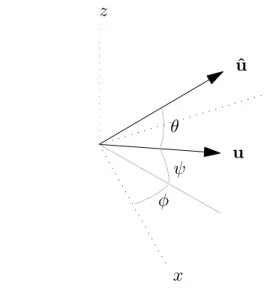
y u x 1 uy ux z uz y ˆ u u ψ x θ φ z

Figure 2.1.1: Unit vectors u and ˆu

by bΘ and Θ. From here I write the signal response and beampattern equations

y = yp · η2_{+ cos(θ)} η2_{+ 1} (2.1.9) B = Bp· ¯ ¯ ¯ ¯η 2 _{+ cos(θ)} η2_{+ 1} ¯ ¯ ¯ ¯ 2 (2.1.10)

where Bp is the beampattern of the associated pressure-sensor array.

Before exploring these expressions in detail, I give a picture of the three-dimensional unit vectors u and ˆu in Figure 2.1.1. The plot on the left illustrates u and its com-ponents in the x, y, and z directions. Note that this unit vector u has an arbitrary direction and need not lie in the x-y plane. The plot on the right shows the same unit vector and the hypothesized direction vector ˆu. I have illustrated the azimuth angle φ and elevation angle ψ of u. I have also illustrated θ, the angle between the two vectors. It is important to understand that θ is the angle between these vectors in R3 _{whereas φ is the angle one vector forms when projected onto the x-y plane.}

From this figure, it is clear that the cos θ term comes from the scalar projection of u onto ˆu.

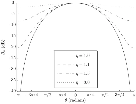
θ (radians) Bv (d B ) −π −3π/4 −π/2 −π/4 0 π/4 π/2 3π/4 π -40 -35 -30 -25 -20 -15 -10 -5 0 η = 1.0 η = 1.1 η = 1.5 η = 3.0

Figure 2.1.2: Vector-sensor modulation term Bv

ulation term Bv , ¯ ¯ ¯ ¯η 2_{+ cos(θ)} η2_{+ 1} ¯ ¯ ¯ ¯ 2 . (2.1.11)

In other contexts, this term is often referred to as the polarization term. This name originates in electromagnetic fields where the additional sensor gain comes from mea-suring wave polarization. Similarly, the angle θ is often called the polarization angle. Figure 2.1.2 plots this term versus θ as the normalization constant η varies. With proper normalization of the data, η = 1, giving the ideal null at θ = ±π. As the vec-tor sensor gain decreases, η → ∞ and Bv → 1, i.e., the vector-sensor array effectively becomes a pressure-sensor array. Also observe that the vector-sensor modulation term varies slowly with θ and forms an envelope for the pressure-sensor beampattern. The “width” of the envelope Bv is generally much larger than the beamwidth of the pressure-sensor array response Bp. Thus, the mainlobe where cos(θ) ≈ 1 is generally dominated by the pressure-sensor response; the vector-sensor terms affects the

side-lobe and ambiguity regions. Put another way, when θ ≈ 0 there is no polarization gain and the vector-sensor array effectively behaves like a pressure-sensor array. As a final note, it is easy to show that any effects from a spatial taper only enter through

Bp and do not alter the vector-sensor term Bv.

2.2

Uniform Linear Array (ULA)

In this section, I apply the results above to the uniform linear array. This simple example illustrates the usefulness of the beampattern factorization and allows me to explore its use in more detail. The uniform linear array considered here is a uniformly weighted array of M linearly spaced sensors separated by d wavelengths. I further assume zero elevation or ψ = 0. Often, I use classical results for the pressure-sensor array which can be found in the thorough source [7].

2.2.1

Beampattern

I now examine in detail the factorization given by Equation 2.1.10. For the uniform linear array defined above, the pressure-sensor beampattern is given by

Bp = 1 M sin h M 2 2πd(cos φ − cos bφ) i sin h 1 22πd(cos φ − cos bφ) i (2.2.1)

and depends on Θ only through the azimuth angle φ. Again, choosing distance d in units of wavelengths greatly simplifies the expressions. Equation 2.2.1 is the familiar discrete sinc or Dirichlet beampattern appearing in classical array literature.

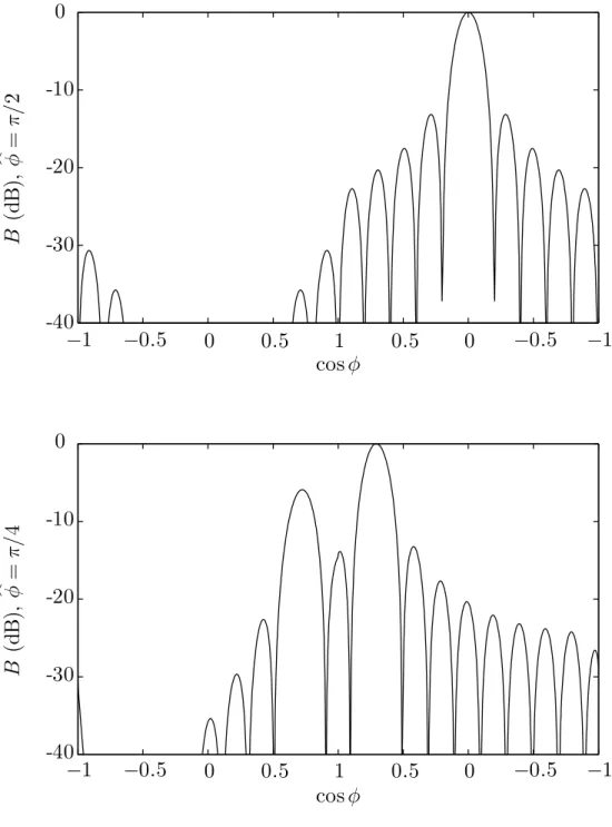
Before illustrating the vector-sensor ULA beampattern, I discuss the coordinate system used in Figures 2.2.1-2.2.3. Although the vector-sensor beampattern is a function of both azimuth and elevation through Bv, I only display a single scan at zero elevation. This is a reasonable restriction when considering sources whose distance is much greater than their depth. As mentioned in Section 1.5, φ = 0 is forward endfire and φ = π/2 is port broadside. The horizontal axis in Figures 2.2.1-2.2.3 scans from

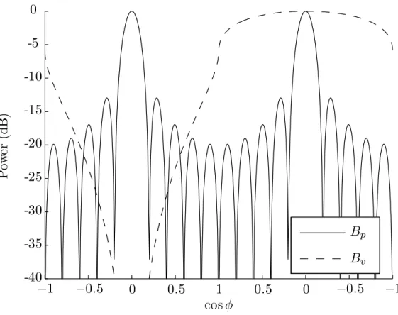
cos φ P ow er (d B ) −1 −0.5 0 0.5 1 0.5 0 −0.5 −1 -40 -35 -30 -25 -20 -15 -10 -5 0 Bp Bv

Figure 2.2.1: ULA Beampattern Components: bφ = π/2

φ = −π to φ = π with constant cosine spacing. Thus, aft endfire is at the left and

right edges and forward endfire is in the center. Also, the starboard side of the array appears on the left half of each plot and the port side appears on the right half. This counterintuitive starboard-to-port scan results from using a right-handed coordinate system with z directed upward.

Now examine the beampattern terms illustrated in Figure 2.2.1 for M = 10,

d = 1/2, and bφ = π/2 (port broadside). Both the pressure-sensor term, Bp, and the vector-sensor modulation term, Bv, for this example are illustrated in Figure 2.2.1. Because it is plotted versus cos φ, the shape of Bv is altered from that in Figure 2.1.2, raising an important distinction: a “natural” parameter space for the pressure-sensor component is cos φ; a “natural” parameter space for the vector-sensor component is θ. In general, ψ 6= 0 and these are different spaces (φ is conical angle but θ is polarization angle in three dimensions).

cos φ P ow er (d B ) −1 −0.5 0 0.5 1 0.5 0 −0.5 −1 -40 -35 -30 -25 -20 -15 -10 -5 0 Bp Bv

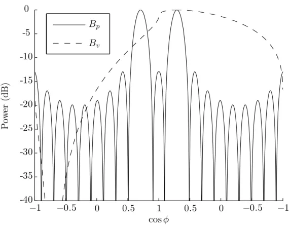
Figure 2.2.2: ULA Beampattern Components: bφ = π/4

Although changing bφ or “steering” with a pressure-sensor array simply shifts the

beampattern in wavenumber space, the same is not true for a vector sensor array. This effect is illustrated in Figure 2.2.2 with bφ = π/4. This figure clearly shows

the left/right, or port/starboard, ambiguity in Bp resulting from the conical angle

φ. Comparing with Figure 2.2.1 reveals a different mapping of the vector-sensor

modulation term. With bφ = π/2 the vector-sensor null lies exactly on an ambiguity

of Bp, but bφ = π/4 produces a null in the sidelobe region.

The beampattern for a vector-sensor array is given by the product of Bp and

Bv. For the examples above with bφ = π/2 and π/4, the beampatterns are shown in Figure 2.2.3. This figure illustrates the effect of the vector-sensors on the left/right ambiguity inherent with the pressure-sensor array. The pressure-sensor ambiguity is nulled when the array is steered to broadside, but it becomes higher as it is steered toward endfire. As before, no spatial taper can further reduce the level of this

cos φ B (d B ), b φ= π / 2 −1 −0.5 0 0.5 1 0.5 0 −0.5 −1 -40 -30 -20 -10 0 cos φ B (d B ), b φ= π / 4 −1 −0.5 0 0.5 1 0.5 0 −0.5 −1 -40 -30 -20 -10 0

sensor ambiguity.

One of the more important theoretical benefits of a vector-sensor ULA is its ability to discriminate acoustic arrivals that would be ambiguous with a pressure-sensor ULA. In the next two subsections, I apply the beampattern factorization in Equation 2.1.10 to study the reduced level of pressure-sensor ambiguities.

2.2.2

Conical Angle (Left/Right) Discrimination

Because a linear pressure-sensor array is symmetric about rotation about its axis, its directional response is a function only of conical angle. This results in ambiguous arrivals: the array cannot determine its left from its right, or port from starboard. In practice, this means the array must maneuver to determine the true location of a source, a strict limitation. As demonstrated in the previous subsection, the velocity components of a vector-sensor array are not symmetric about any rotation. As a result, a linear vector-sensor array may “resolve” ambiguities that would be present with a pressure-sensor array.

With a linear pressure-sensor array, a source arriving at the hypothesized angle b

φ is indistinguishable from a source at angle φ0 _{= 2π − bφ, the same conical angle} on the opposite side of the array. This ambiguity produces a peak or “backlobe” in the beampattern. Because the angle of these sources in three dimensions - the polarization angle θ - is clearly different, they are unambiguous with a vector-sensor array. In terms of the beampattern equations, this means

Bp(bφ) = Bp(φ0) = 1 (2.2.2)

The directional response at the backlobe φ0 _{is given by} B(φ0_{) = B} v(φ0) = ¯ ¯ ¯ ¯ ¯ η2_{+ cos(bφ − φ}0₎ η2_{+ 1} ¯ ¯ ¯ ¯ ¯ 2 = ¯ ¯ ¯ ¯ ¯ η2_{− 1 + 2 cos}2_(bφ) η2_{+ 1} ¯ ¯ ¯ ¯ ¯ 2 (2.2.4)

where the last step substitutes for φ0 _{and applies a double angle identity. With proper} normalization of the data, η = 1, resulting in the simple but useful relation

B(φ0) = cos4(bφ) (2.2.5)

giving the left/right suppression for any steering angle bφ. Note that although φ0 _{is an} ambiguity for the pressure sensor array, it is not necessarily the highest point in the beampattern of a vector sensor array. One such example is Figure 2.2.3 for bφ = π/4.

The vector-sensor modulation shifts the peak of the backlobe very slightly toward endfire. In practice, Equation 2.2.5 is a good approximation to the peak value when the mainlobe is not excessively large. It is also important that the level and location of the backlobe are not affected by any spatial taper and do not vary with frequency or the number of sensors.

One use of Equation 2.2.5 is to give approximate regions over which a given left/right resolution is obtained: for at least 6 dB of resolution, π/4 ≤ bφ ≤ 3π/4 or

within π/4 radians of broadside.

2.2.3

Spatial Aliasing (Grating Lobe) Discrimination

In the same way that under-sampling a time signal produces frequency aliasing, spa-tially under-sampling a plane wave produces aliasing in the beampattern. The ambi-guities or “grating lobes” resulting from this spatial aliasing limit the use of pressure-sensor arrays above a given design frequency. To further illustrate the usefulness of the beampattern results shown above, I quickly derive expressions for the location

and level of pressure-sensor grating lobes on the uniform linear vector-sensor array. One theoretical benefit to acoustic vector-sensor arrays is their improved perfor-mance above the design frequency of corresponding pressure-sensor arrays. The design frequency of a uniform linear array is analogous to the Nyquist frequency for spatial sampling. Using previous notation, the perfect reconstruction criterion is d < 1/2. Denoting the inter-element spacing by δ units of length (whereas d is in wavelengths), this gives the design frequency

fd=

c

2δ. (2.2.6)

The spatial aliasing occurring above this design frequency enters only through Bp (Equation 2.2.1) because this function is periodic with respect to cos φ. In the follow-ing analysis I restrict my attention to pressure-sensor gratfollow-ing lobes existfollow-ing within acoustic space. By symmetry, it is sufficient to consider only arrival angles bφ < π/2.

The location of the pressure-sensor grating lobes is then easily found as

cos φ0 = cos bφ − 1 d

= cos bφ − 2fd

f . (2.2.7)

Examining this expression quickly reveals that the location of a pressure-sensor grat-ing lobe depends on both arrival angle and analysis frequency. Even above the design frequency, pressure-sensor grating lobes for some angles bφ may not exist in physical

space. Like the backlobes in the previous subsection, Bp(φ0) = 1, leaving

B(φ0_{) = B} v(φ0) = 1 (η2_{+ 1)}2 ¯ ¯ ¯ ¯η2+ cos · b φ − cos−1 µ cos bφ − 2fd f ¶¸¯_¯ ¯ ¯ 2 . (2.2.8)

Unlike the backlobe expression in Equation 2.2.5, Equation 2.2.8 is clearly dependent on frequency. Both results, however, are independent of the number of sensors and any spatial tapering. This leads to the important conclusion that neither backlobe nor grating lobe reduction is enhanced by increasing the number of sensors.

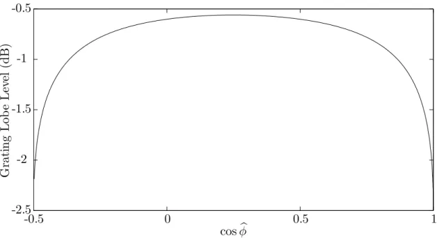
cos bφ G rat in g Lob e Le ve l (d B ) -0.5 0 0.5 1 -2.5 -2 -1.5 -1 -0.5

Figure 2.2.4: Vector-sensor “Grating Lobe” Height: f /fd= 4

provide some insight. In the examples to follow, I again assume that η = 1. First, I fix the frequency at f /fd = 4 and examine the “grating lobe” levels across all bφ. I again put the term in quotations because spatially aliased sources are no longer ambiguous on a vector-sensor array and thus not true grating lobes. The result is shown in Figure 2.2.4. For this figure, the input range is restricted to cos bφ ∈ [−1/2, 1]

because no “grating lobes” occur in acoustic space when cos bφ < −1/2. As a second

example, I fix the angle at broadside, bφ = π/2, and consider the “grating lobe”

level as a function of frequency. At this angle, “grating lobes” begin to appear when

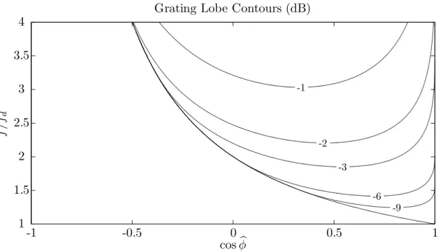
f /fd≥ 2. As is shown in Figure 2.2.5, these lobes are at a −6 dB level when they first appear at twice the design frequency. As a final example, I plot contours of Equation 2.2.8 versus bφ and f /fd. These contours are shown in Figure 2.2.6. The unlabeled contour corresponds to the angle beyond which no “grating lobes” appear in acoustic space. Figure 2.2.6 is readily used for design and analysis; for example, if an adaptive beamforming algorithm effectively nulls signals with 3 dB of mismatch, it may null these “grating lobes” up to approximately twice the design frequency.

f /fd G ra ti n g Lob e L ev el (d B ) 2 2.5 3 3.5 4 -7 -6 -5 -4 -3 -2 -1 0

Figure 2.2.5: Vector-sensor “Grating Lobe” Height: bφ = π/2

cos bφ

f

/f

d

Grating Lobe Contours (dB)

-1 -2 -3 -6 -9 -1 -0.5 0 0.5 1 1 1.5 2 2.5 3 3.5 4

2.2.4

Near-Field Processing

Although the factorization given in Equation 2.1.10 is helpful for plane wave signals, it also holds well as an approximation when wavefront curvature increases. The “far-field” or plane-wave assumption that allows factoring the vector sensor term out of the array response is more strict than the traditional Fresnel rule-of-thumb. The Fresnel far-field distance for an array of aperture size L, usually given as df f = L2/2λ, is based on a maximum phase error of π/8 [8]. With geophones, however, the angle-of-arrival error at the aperture edges produces differences in the beampattern at ranges greater than df f. At first glance, this seems to limit the practical use of Equation 2.1.10. However, this approximation is still useful because it may begin failing in the low sidelobe regions. These regions, although of theoretical interest, may already be unattainable in practice and may not contribute much integrated error. Because this thesis deals only with plane wave signals, a more detailed discussion of near-field effects is outside its scope.

Chapter 3

Mismatched Vector-Sensor Arrays

In the previous chapter, I considered “ideal” vector-sensor arrays. I term these arrays “ideal” because of two strong assumptions. First, I assume there are no errors in the model, i.e. the sensor positions and orientations are known. Second, I assume the received signal is deterministic and without sensor noise. In practice, both of these assumptions are typically violated. Sometimes, the sensor parameters - position and orientation - are fixed and known with some error tolerance. With other arrays, the sensor parameters vary slowly with time and can only be approximated. Signals, in practice, are usually embedded in noise and modeled stochastically.

This chapter expands my analysis to include these practical considerations. Of pri-mary concern is the performance of acoustic vector-sensor arrays under “mismatch” or modeling errors. Now that I know how well “ideal” vector-sensor arrays can do, how does their performance degrade when the sensor parameters have random errors? The first section below considers the uniform linear array under Gaussian perturba-tions. Using some results from nonuniform sampling theory, it computes the average beampattern and studies the effects introduced by mismatch. The second section ex-amines the problem of direction-of-arrival (DOA) estimation. With a Gaussian signal and error model, it derives and analyzes a Cram´er-Rao lower bound for any unbiased DOA estimator.

3.1

Perturbed Linear Array

The previous chapter derived a simple form (see Equations 2.1.10 and 2.2.1) for the beampattern of a uniform linear array of vector-sensors. Before delving into direction-of-arrival estimation, it would be useful to understand how this beampattern changes when the array parameters have random errors. To keep the analysis simple, I consider only independent identically distributed (IID) Gaussian position errors. For a more detailed analysis of the beampattern under Gaussian modeling errors - including rotation, gain, and phase errors - see the work in [3] and [9]. Also, for an alternate analysis of random pressure-sensor arrays, see [10].

In the following subsections, I only consider the effect of position errors on the pressure-sensor array beampattern Bp. To motivate this discussion and justify ignor-ing the vector-sensor term Bv, examine the mean vector-sensor array beampattern with position errors only. I denote expectation with E{·} and use the random vector

ρR _{to represent the position errors. Suppressing the dependence on bΘ, the expected} beampattern is then

E{B} = E_ρR{B_p · B_v}

= E_ρR{B_p} · B_v (3.1.1)

where the factorization is possible because Bv is a function of known rotation param-eters only and Bp is a function of position parameters only. When rotation errors are also considered as in [3], this factorization is not possible. As I show in this section, focusing on such a simplified model allows me to connect the field of “nonuniform sampling” to the analysis of a perturbed linear array. Although the resulting proof is less general the one given in [9], it is more insightful thanks to the connections with nonuniform sampling.

3.1.1

Nonuniform Sampling

Before analyzing the perturbed linear array, I briefly state a useful result from the nonuniform sampling of a signal. The signal I define is the wide-sense stationary continuous-time random process f (t). This signal is sampled at nonuniform times to give ˜f [n] = f (nT +ξn) where T is the nominal sampling period and ξnis a sequence of IID random variables. Recent work presented in [11] relates the discrete-time power spectrum density (PSD) S_{f ˜}˜_f to the continuous-time PSD Sf f:

S_{f ˜}˜_f ¡ ejω¢ ₌ 1 T ∞ X k=−∞ Sf f µ ω − 2πk T ¶ ¯_¯ ¯ ¯ϕξ µ ω − 2πk T ¶¯_¯ ¯ ¯ 2 + 1 2π Z _∞ −∞ Sf f(Ω) £ 1 − |ϕξ(Ω)|2 ¤ dΩ (3.1.2) where ϕξ(s) = E ©

ejsξª _{is the characteristic function of ξ. Stating this result in} words, the nonuniform sampling causes two effects: 1) the continuous-time PSD is windowed by ϕξ and aliased, and 2) white noise is introduced. Also note that with uniform sampling ϕξ = 1 and Equation 3.1.2 reverts to the standard uniform sampling expression for aliasing.

3.1.2

Relation to Perturbed ULA

To connect Equation 3.1.2 with the perturbed linear array, I must introduce the concept of an infinite linear aperture. The linear array obtains measurements at a finite number of points on a line, but an infinite linear aperture obtains measurements at every point on the line. Without loss of generality, assume the infinite linear aperture is oriented along the x axis and the single source is in the x-y plane. I now define

k0 ,

2π

λ (3.1.3)

In words, the variable k0 is the magnitude of the wavenumber and kx is the

wavenum-ber component along the array axis. The infinite linear aperture measurements are of acoustic pressure in phasor form, written as

p(x) = exp

³

j bkx x ´

. (3.1.5)

Because this array lies in the same x-y plane as the propagating wave, I need only consider position errors in the x and y directions. To formalize the modeling errors, assume the position perturbations are zero-mean Gaussian with variances given by

σ2

x and σy2.

Having now defined an infinite linear aperture, I examine its relationship to nonuniform sampling. Using the same notation as Section 3.1.1, the discrete sensors with position perturbations are equivalent to a finite nonuniform spatial sampling of

p(x). Specifically, I write the discrete measurements as a_pn = p(nδ + ξn), where ξn are zero-mean Gaussian IID random variables with variance σ2 _{= σ}2

x+ σ2ytan2φ. Col-b lapsing the position errors into a single variance is possible because errors along the

y axis are equivalent to scaled errors along the x axis. Now, I relate time in Equation

3.1.2 to space along the infinite linear aperture. Formally, this means variables are remapped like

t ↔ x

Ω ↔ kx

. (3.1.6)

Now the importance of wavenumber kx is clear: it is the spatial equivalent to angular frequency Ω.

To show the implications of this mapping from time to space, I apply the nonuni-form sampling result to the perturbed array in four steps. The first step simply maps variables from space to time. This mapping gives the equivalent time series

f (t) = p(t) which is now sampled at intervals equal to the inter-element spacing T = δ. The second step computes the terms in Equation 3.1.2. The time series is

simply a complex exponential and the ξn are Gaussian, so I have Sf f(Ω) = 2πD ³ Ω − bkx ´ (3.1.7) |ϕξ(Ω)|2 = exp ¡ −σ2_Ω2¢ _(3.1.8)

where D(·) is the familiar Dirac delta function. The sifting property of the delta function makes the evaluation of Equation 3.1.2 simple, giving

γ , exp ³ −σ2 _bk2 x ´ (3.1.9) = exp h −k2 0 ³ σ2 xcos2φ + σb y2sin2φb ´i (3.1.10) S_{f ˜}˜_f ¡ ejω¢ ₌ 2πγ δ ∞ X k=−∞ D µ ω − 2πk δ − bkx ¶ + (1 − γ) . (3.1.11)

Note that S_{f ˜}˜_f is the PSD for an infinite-length sequence of samples. To reflect the

finite number of samples in a linear array, the third step windows this sequence. I now define w[n] ,    1/M 0 ≤ n < M 0 otherwise (3.1.12) g[n] , w[n]f (nδ) (3.1.13) ˜g[n] , w[n] ˜f [n] (3.1.14)

where the rectangular window w[n] is normalized to agree with Equation 2.1.2. Note that g[n] is the sequence obtained by uniform sampling and ˜g[n] is the sequence obtained by nonuniform sampling. Through linearity, windowing the first term in Equation 3.1.11 gives γ times the uniform sampling PSD. The second term gives white noise that is easily evaluated in the time domain. Combining the two produces

Sg˜˜g ¡ ejω¢_{= γ · S} gg ¡ ejω¢_{+ (1 − γ) ·} 1 M. (3.1.15)

a result in terms of φ. The PSD of g[n] becomes the nominal beampattern and the PSD of ˜g[n] becomes the expected beampattern. After the transformation, Equation 3.1.15 becomes

E{Bp( φ )} = γ · Bp( φ ) + (1 − γ) · 1

M. (3.1.16)

Note that the derivation above is easily extended to non-rectangular windows and is valid as stated for any window normalized for unity gain. Note also that it is trivial to include Gaussian phase errors in the proof through Equation 3.1.10.

3.1.3

Analysis of the Expected Beampattern

Although the end result in Equation 3.1.16 is the same as that derived in [9] for a nominally linear array, the derivation shown here has two benefits. First, it connects the field of array processing to that of nonuniform sampling. Linear arrays have long been associated with discrete-time signal processing, but they have not been fully explored in the context of nonuniform sampling. Though the end result in [9] has a nice interpretation, the proof is strictly mathematical. A second benefit of my derivation is that it comes with an intuitive picture of how position mismatch affects the beampattern.

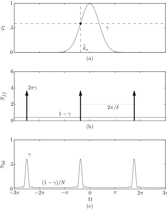
To gain this intuition, examine Figure 3.1.1. This figure results from the param-eters M = 16, f = 2fd, bφ = 4π/9, σx = λd/3, and σy = 0. Each illustration is shown on the same horizontal axis of Ω, analogous to the horizontal wavenumber kx. Part (a) of the illustration shows the characteristic function ϕξ. As shown by the dotted lines, the mismatch factor γ comes from this curve evaluated at the source wavenumber bkx. Because the position errors are Gaussian, ϕξ takes a normalized Gaussian shape. As position errors decrease, the characteristic function spreads and γ increases. Part (b) shows the PSD S_{f ˜}˜_f of the nonuniformly sampled infinite sequence ˜f [n]. Compared to

an uniformly sampled PSD, the impulse train is weighted by a factor of γ and white noise of power 1 − γ is added. In the limit of no mismatch the PSD converges to the familiar impulse train. Part (c) shows the effect of windowing the sequence ˜f [n] to

b kx γ (a) ϕξ 0 .5 1 2πγ 1 − γ 2π/δ (b) S˜ f ˜ f 0 2 4 6 γ (1 − γ)/N Ω (c) S˜g ˜g −3π −2π −π 0 π 2π 3π 0 .5 1

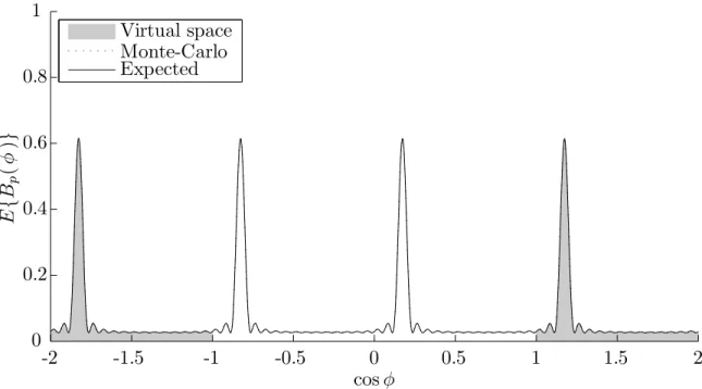
cos φ E { Bp ( φ )} -2 -1.5 -1 -0.5 0 0.5 1 1.5 2 0 0.2 0.4 0.6 0.8 1 Virtual space Monte-Carlo Expected

Figure 3.1.2: Mismatched Beampattern: f = 2fd

S_{f ˜}˜_f yielding a Dirichlet function.

To complete the picture of position mismatch, the PSD in Figure 3.1.1 must be mapped from Ω to φ. By definition, Ω ↔ kx and kx = −k0cos φ so a region of Ω

maps linearly to a region in cos φ. Figure 3.1.2 shows this mapping for the illustrated example in the previous paragraph. I have also included the average beampattern from a 4000-trial Monte-Carlo simulation although it lies almost exactly on the pre-dicted curve. The shaded region corresponding to cos φ /∈ [−1, 1] is dubbed “virtual

space” because no real φ maps to this region. The term “physical space” likewise refers to the complementary region of real φ. Because the analysis frequency is above the design frequency of the array more than one peak maps into physical space. This produces spatial aliasing, or grating lobes, in the beampattern. If I lower the analysis frequency to f = fd/2 but keep the same source wavenumber bkx and mismatch σ, the illustration in Figure 3.1.1 remains exactly the same. The mapping to φ, however, changes as shown in Figure 3.1.3. Because the new analysis frequency is below the array design frequency only one peak maps into physical space and no grating lobes are present.

cos φ E { Bp ( φ )} -2 -1.5 -1 -0.5 0 0.5 1 1.5 2 0 0.2 0.4 0.6 0.8 1 Virtual space Monte-Carlo Expected

Figure 3.1.3: Mismatched Beampattern: f = fd/2

The decrease in peak value caused by mismatch is simply a factor γ which in decibels grows linearly with σ2b_k2

x. The expected beampattern is a linear interpolation between the ideal beampattern and 1/M white noise - with γ as the interpolation factor. Having derived some intuition for the expected beampattern under position errors only, I now examine the vector-sensor array performance under a more general class of modeling errors.

3.2

Cram´

er-Rao Bound

This section derives a Cram´er-Rao bound for direction-of-arrival estimation error with a single-source. The initial model is an arbitrary array of vector sensors whose position and rotation are perturbed by zero-mean Gaussian errors. Later subsections extend this model to include Gaussian gain and phase errors. The modeling errors here are the same as in [3] and are a vector-sensor extension of the Gilbert-Morgan model in [9]. Despite sharing a mismatch model, the DOA bound explored in this thesis is distinct from the beampattern expressions derived in [3]. All measurements under this model are of a zero-mean Gaussian random process of unknown power corrupted by additive white noise of unknown power. This is the more common scenario of “unknown signal in unknown noise.” To keep things shorter I use without proof the “hybrid” Cram´er-Rao bound given in [7], Chapter 8.11. The bound used below is an approximation that is valid when the variance of the perturbations is small (again, see [7]). Note also that without modeling errors this bound reduces to the result given in [2].

3.2.1

Statement of the Hybrid Bound

The stochastic model outlined above may seem simple, but the bound it produces is quite complex to derive and express. This subsection elaborates on the model, defines several useful quantities, and states the hybrid Cram´er-Rao bound explored in the rest of the chapter. It also clarifies some notation in an attempt to keep the derivation as simple as possible.

I begin by defining some helpful quantities and notation. Recalling the plane wave replica vector v parameterized by Θ = [φ ψ]T_{, suppose there are K independent} measurements or “snapshots” of the form

xk(Θ) = v(Θ) · CN (0, σ2s) + CN (0, σn2), k = 1, 2, . . . , K (3.2.1)

variance σ2_{. If the noise variance of the pressure sensors differs from that of the}

velocity sensors, it can be absorbed without loss of generality into the normalization constant η. This normalization introduced in Equation 1.5.7 allows me to treat the sensors as having equal noise powers. As stated above, my model assumes the more common scenario where both variances σ2

s and σn2 are unknown. Also, each vector-sensor is perturbed by Gaussian position and rotation errors. It is further assumed that the components of each vector-sensor are rigidly connected and thus displaced and rotated together. To help keep a simple notation, I use a semicolon to denote vertical concatenation. I then define the perturbation parameters in column vectors

ρR _{, [x ; y ; z] (3.2.2)}

ρΘ _{, [α ; β ; γ] (3.2.3)}

ρ , £ρR _{; ρ}Θ¤ _(3.2.4)

where ρR _{are the Euclidean coordinates of a sensor and ρ}Θ _{are the Euler rotation}

angles about the corresponding coordinate axes. I also introduce notation to index into the source and rotation parameters, using Θland ρl to indicate the lth parameter in Θ and ρ, respectively. This is a slight abuse of notation because each vector-sensor technically has its own perturbation parameters. For the mth vector-sensor, I denote these perturbation parameters by {xm, ym, zm, αm, βm, γm}. In the results that follow, I often find block matrices that cannot be expressed simply with Kronecker and Hadamard products. With such matrices, notation like A = [Aij] indicates that the terms Aij are concatenated over row index i and column index j to form the matrix A. Another example of this notation is [∂A/∂ρi], indicating the vertical concatenation of the derivatives of the matrix A with respect to the perturbation parameters ρ.

Having setup some notation and defined the model parameters, I begin listing terms used in the following sections. First, I define the derivative of the replica

vector with respect to the source parameters

Dφ ,

∂v

∂φ, etc. (3.2.5)

DΘ , [Dφ Dψ] (3.2.6)

where “etc.” indicates that Dψ is defined similarly. Because v is a length 4M column vector, Dφis 4M ×1 and DΘ is 4M ×2. I also create derivatives of a slightly different

form with respect to the perturbation parameters

Dx , · ∂v1 ∂x1 ; ∂v2 ∂x2 ; . . . ; ∂v4M ∂x4M ¸ , etc. (3.2.7)

where the derivatives in Equation 3.2.7 go through all 4M sensor elements (M pressure sensors and 3M velocity sensors as defined in Equation 2.1.1). Just as D? defined derivatives of the replica vector v with respect to a given variable ?, the notation δ? defines derivatives of the unit vector u:

δφ,

∂u

∂φ, etc. (3.2.8)

Another helpful notation is to define derivatives of the h vector similarly

∆φ,

∂h

∂φ, etc.1 (3.2.9)

From the results from Section 2.1 recall that vH_{v = M(η}2_{+ 1). In keeping with the}

1_{For the derivatives considered, ∆}

notation from [7], I define the terms Sf , σ2s (3.2.10) Sx , vSfvH + σn2I (3.2.11) Σ , SfvHS−1x vSf/σ2n = σ2 svH £ vvH_σ2 s+ σn2I ¤−1 vσ2 s/σ2n = γ2_vH£_γvvH _{+ I}¤−1_v = γ2_vHh_{I − γv}¡_{1 + γv}H_v¢−1_vHi_v = γ2_vH_v µ 1 − γvHv 1 + γvH_v ¶ = γ · γM (η 2_{+ 1)} γM (η2_{+ 1) + 1} (3.2.12) where γ = σ2

s/σn2 is the element signal-to-noise ratio (SNR).2 Note that Sf and Σ are scalar values because of the single source. Lastly, I define

P⊥

v , I − v(vHv)−1vH

= I − [(apaHp ) ⊗ (hhH)]/[M(η2+ 1)], (3.2.13)

a projection matrix orthogonal to the replica subspace. In other words, the source replica vector v spans the nullspace of the projection matrix P⊥

v. This matrix can be

viewed as a covariance matrix driving a perfect null in the direction of the source. With the above definitions, I now state the hybrid Cram´er-Rao bound. To simplify the resulting equation, I write it in block form and in terms of the matrices

A , 2KΣ · Re©DH ΘP⊥vDΘ ª (3.2.14) B , 2KΣ · Re nh (P⊥ v)TD∗Θj ¯ Dρi io (3.2.15) C , 2KΣ · Re nh D_ρiDH ρj ¯ (P⊥v)T io + Λ−1 ρ . (3.2.16)

2_{This Σ is not exactly the same as that used in [7]. Here, it has a nice interpretation as the}

In the above equations, ∗ _{denotes matrix conjugation. The covariance matrix Λρ} specifies the second-order statistics for the perturbation parameters. Again using notation similar to [7], the following equation for CHCR lower bounds the mean-square error of unbiased estimates for Θ and ρ:

CHCR(Θ, ρ) =   A B T B C   −1 . (3.2.17)

For the remainder of this section, I only consider the mean-square error bounds on the source parameters Θ. That is, I treat the perturbations ρ as nuisance parameters. This allows me to rewrite Equation 3.2.17 for only the upper left partition as

CHCR(Θ) = £

A − BTC−1B¤−1. (3.2.18)

This form of the hybrid Cram´er-Rao bound is presented in more detail in [7]. Al-though Equation 3.2.18 bounds estimation of Θ in radians, it is often better to know the bound in cosine-space. Thankfully, applying a simple change of coordinates to the CRB is easily done as described in [7]. For the bound on φ this only requires multiplying by sin2_{φ. Keeping Equation 3.2.18 in mind, I now begin evaluating the}

terms of the bound in detail.

3.2.2

Evaluation of Terms

When deriving each term in the hybrid Cram´er-Rao bound, a few observations become very helpful. First, the real components in h are unaffected by position errors. Put another way, only the phase vector ap is affected when perturbing the sensor positions. Second, the phase components in ap are unaffected by orientation errors. The two statements above are another instance where the factorization in Equation 1.5.7 comes in very handy: position errors enter through ap and rotation errors enter through h. Evaluation of Equation 3.2.18 begins in the logical place with the matrix A. For

this, I need the derivatives that compose DΘ: Dφ = ∂ ∂φv = ∂ ∂φ(ap⊗ h) = ∂ap ∂φ ⊗ h + ap⊗ ∂h ∂φ = ¡j2πRTδφ¯ ap ¢ ⊗ h + ap⊗ ∆φ (3.2.19)

where R , [r1 r2 . . . r4M] is a matrix containing the element positions in units of

wavelengths. The first term in Equation 3.2.19 is the derivative of the phase compo-nent; the part in parentheses is the equivalent derivative for a pressure-sensor array. The second term is the corresponding derivative for the directional gain. Similarly, the elevation derivative is

Dψ =¡j2πRTδψ¯ ap ¢

⊗ h + ap⊗ ∆ψ. (3.2.20)

It is now easy to calculate the derivatives of the unit vector u as defined in Equation 3.2.8:

δφ = [− sin φ cos ψ ; cos φ cos ψ ; 0] (3.2.21)

δψ = [− cos φ sin ψ ; − sin φ sin ψ ; cos ψ] . (3.2.22)

Without loss of generality, I assume the origin of the coordinate system is the ar-ray centroid. As was mentioned in [2], the three vectors {u , δφ , δψ} are or-thogonal as illustrated in Figure 3.2.1. From this, it is easy to see that the vec-tors {h , ∆φ , ∆ψ} are also orthogonal. Their orthogonality along with the choice of origin implies DH

u ψ φ y x z δφ u δψ y x z

Figure 3.2.1: Orthogonal Vectors {u , δφ , δψ}

Equation 3.2.14 above gives

A = 2KΣ · Re©DH ΘDΘ ª = 2KΣ · Re      DHφDφ DHφDψ DH ψDφ DHψDψ     . (3.2.23)

I now evaluate the terms in this matrix, starting with the off-diagonal term

DH φDψ = ©¡ j2πRT_δ φ¯ ap ¢ ⊗ h + ap⊗ ∆φ ª_H ©¡ j2πRT_δ ψ ¯ ap ¢ ⊗ h + ap⊗ ∆ψ ª = ©¡j2πRT_δ φ¯ ap ¢ ⊗ hªH©¡j2πRT_δ ψ ¯ ap ¢ ⊗ hª + {ap⊗ ∆φ}H{ap⊗ ∆ψ} = 4π2_(η2_{+ 1) · δ}T φ(RRT)δψ+ M · δφTδψ. (3.2.24) The first step above eliminates the cross-terms because the vectors {h , ∆φ , ∆ψ} are orthogonal; the second step substitutes the norms of ap and h. Modifying

Equation 3.2.24, I easily get the remaining terms to yield the simplified form A = 2KΣ   4π 2_(η2_{+ 1)}   δφT(RRT)δφ δφT(RRT)δψ δT φ(RRT)δψ δψT(RRT)δψ   + M   cos2ψ 0 0 1      (3.2.25)

which is the same expression given in [2] when there is no position or orientation uncertainty. The second term in this equation contains the inner products of the orthogonal vectors δφ and δψ and is thus diagonal. It is also easy enough to see that the second term in Equation 3.2.24 combines with the first to give

A = 2KΣ · [δφ δψ]T ©

4π2_(η2_{+ 1) · RR}T _{+ M · I}ª_[δ

φ δψ]. (3.2.26)

This representation is appealing because the array geometry only enters through the term in curly brackets, specifically through RRT_{. Likewise, the source position only} enters through the matrix term [δφ δψ].

Having derived an expression for A, I move to the next term B. Recall that the paragraph above showed DH

ΘP⊥v = DHΘ. Using this, I now seek the simpler but

equivalent expression B = 2KΣ · Re nh D∗_Θj ¯ D_ρi io . (3.2.27)

Because the B matrix is in block form, I begin by looking at a single block term D∗

φ ¯ Dx. Having already computed Dφ above, I start with Dx. Although Dx is

defined in Equation 3.2.7 using derivatives of each of the 4M sensor elements, it is easier to consider the derivative taken over each of the M vector-sensors. For the kth vector-sensor, ∂vk ∂xk = ∂ ∂xk (apk ⊗ h) = h · ∂ ∂xk exp©j2π(rT_ku)ª = j2πux· vk (3.2.28)

where ux is the x-component of the unit vector u. To make the first step shown, I use the property described above: the vector h is invariant with respect to changes in position. Applying this result to every vector-sensor makes the complete derivative

Dx = · ∂v1 ∂x1 ; ∂v2 ∂x2 ; . . . ; ∂vM ∂xM ¸ = j2πux· v (3.2.29)

with similar results for Dy and Dz. Denoting an M-length vector of ones with 1M, I now compute the element-wise product

D∗ φ¯ Dx = ©¡ j2πRT_δ φ¯ ap ¢ ⊗ h + ap⊗ ∆φ ª_∗ ¯ {j2πuxap⊗ h} = ¡4π2_u xRTδφ¯ a∗p¯ ap ¢ ⊗ (h ¯ h) + ¡j2πuxa∗p¯ ap ¢ ⊗ (h ¯ ∆φ) = ¡4π2_u xRTδφ ¢ ⊗ (h ¯ h) + (j2πux1M) ⊗ (h ¯ ∆φ) (3.2.30)

where the first step applies the Kronecker mixed-product property and the second uses the identity a∗

p ¯ ap = 1M. Since I am only interested in the real part of this result, I need only the first term in Equation 3.2.30,

Re©D∗ φ¯ Dx

ª

= 4π2_u

xRTδφ⊗ (h ¯ h) . (3.2.31) From this result, it is easy to extrapolate every analogous term with {Dx, Dy, Dz}

and with Dψ. The only remaining terms are those involving the rotation parameters such as D∗

φ¯ Dα. When I computed the position perturbation terms {Dx, Dy, Dz},

I simply differentiated with respect to existing position parameters rk. To follow the same procedure for the rotation parameters, I incorporate a rotation matrix about the three axes, Q(α, β, γ)T. Suppressing the arguments of Q, substitute the rotated

vector h = [η ; QT_{u] and write}3 ∆α = " 0 ; µ ∂Q ∂α ¯ ¯ ¯ ¯ α=0 ¶_T u # . (3.2.32)

Using the same rotation matrix, analogous expressions result for ∆β and ∆γ. An expression for the rotation matrix may be easily found elsewhere, but I list the ∆? terms for convenience

∆α = [0 ; 0 ; sin ψ ; − sin φ cos ψ] (3.2.33) ∆β = [0 ; − sin ψ ; 0 ; cos φ cos ψ] (3.2.34) ∆γ = [0 ; sin φ cos ψ ; − cos φ cos ψ ; 0]. (3.2.35)

Using these derivatives, computing one rotation perturbation term gives

∂vk ∂αk = ∂ ∂αk (apk⊗ h) = apk ⊗ ∆α (3.2.36) ∴ Dα = ap⊗ ∆α. (3.2.37)

I can now express the element-wise product

D∗ φ¯ Dα = ©¡ j2πRT_δ φ¯ ap ¢ ⊗ h + ap⊗ ∆φ ª∗ ¯ {ap⊗ ∆α} = ¡−j2πRT_δ φ¯ a∗p¯ ap ¢ ⊗ (h ¯ ∆α) + ¡a∗ p¯ ap ¢ ⊗ (∆α¯ ∆φ) = ¡−j2πRT_δ φ ¢ ⊗ (h ¯ ∆α) + (1M) ⊗ (∆α¯ ∆φ) . (3.2.38)

As before, I am only interested in the real part

Re©D∗ φ¯ Dα

ª

= (1M) ⊗ (∆α¯ ∆φ) . (3.2.39)

3_{Because the nominal rotations are zero, this is simply a more verbose definition of h and does}

Enough representative terms have been derived now to write the matrix B: B = 2KΣ ·               4π2_u xRTδφ⊗ (h ¯ h) 4π2uxRTδψ ⊗ (h ¯ h) 4π2_u yRTδφ⊗ (h ¯ h) 4π2uyRTδψ⊗ (h ¯ h) 4π2_u zRTδφ⊗ (h ¯ h) 4π2uzRTδψ⊗ (h ¯ h) 1M ⊗ (∆α¯ ∆φ) 1M ⊗ (∆α¯ ∆ψ) 1M ⊗ (∆β¯ ∆φ) 1M ⊗ (∆β¯ ∆ψ) 1M ⊗ (∆γ¯ ∆φ) 1M ⊗ (∆γ¯ ∆ψ)               = 2KΣ ·   4π2u ⊗ (RT[δφ δψ]) ⊗ (h ¯ h) [ 1M ⊗ (∆ρΘ i ¯ ∆Θj) ]   _(3.2.40)

where the lower term in the last equation is itself a block matrix.

Having derived expressions for the matrices A and B, I naturally turn to the final block C in the hybrid Cram´er-Rao bound. For convenience, I restate the definition in Equation 3.2.16: C , 2KΣ · Re nh D_ρiDH_ρj ¯ (P⊥_v)T io + Λ−1_ρ .

Having already computed the derivatives D? needed, I immediately begin computing a single term D_xDH y ¯ (P⊥v)T = (j2πuxv)(j2πuyv)H ¯ (P⊥v)T = 4π2_u xuyvvH ¯ (P⊥v)T = 4π2_u xuy(apaHp ⊗ hhT) ¯ (P⊥v)T. (3.2.41)

Although it may not be immediately obvious, this term itself is real, so taking the real part is not necessary. Analogous results follow for the other position perturbation blocks. Looking at a rotation perturbation block gives

D_αDH_β ¯ (P⊥_v)T = (ap⊗ ∆α)(ap⊗ ∆β)H ¯ (P⊥v)T

which again is a real matrix. Finally, the off-diagonal blocks in the C matrix are terms like

D_xDH_α ¯ (P⊥_v)T = (j2πuxap⊗ h)(ap⊗ ∆α)H ¯ (P⊥v)T

= j2πux(a_paH_p ⊗ h∆T_α) ¯ (P⊥_v)T. (3.2.43)

Although the diagonal blocks were real, these terms are purely imaginary. Because their real part is zero, these blocks form matrices of zeros in C. Writing all blocks together and simplifying gives

C1,1 , 4π2uuT ⊗ £ vvH _{¯ (P}⊥ v)T ¤ (3.2.44) C2,2 , h (a_paH p ⊗ ∆ρΘ i ∆ T ρΘ j) ¯ (P ⊥ v)T i (3.2.45) C = 2KΣ ·   C1,1 0 0 C2,2   + Λ−1 ρ . (3.2.46)

Although this expression can be expanded, I keep it in this form for brevity.

Having now computed enough terms to evaluate the hybrid Cram´er-Rao bound, a few notes are worth mentioning. First, if any perturbations are deterministic or zero, they introduce singularities into the bound. Put another way, deterministic errors should not be included in the CRB. If any perturbation is nonrandom, the corresponding row and column in C−1

HCR should be removed. See [7] for more details and an example. Second, the rotation perturbations for each pressure sensor may be modeled as zero. Based on discussions above, the pressure sensor measurements do not depend on orientation. Combined with the first point, this means I could remove the rows and columns in B and C corresponding to pressure sensor rotation errors. Third, the vector-sensor array deteriorates into a pressure-sensor array as η → ∞. This means that much of the work I have done, including the CRB, is valid for a pressure-sensor array if I let η → ∞. Equivalently, to bound a pressure-sensor array I can let h = [ 1 ; 0 ; 0 ; 0 ] or the scalar h = 1, although these require changing many of the derivatives I have computed. Thus, the CRB bound on DOA estimation