Aggregate investment

Digitized

by

the

Internet

Archive

in

2011

with

funding

from

Boston

Library

Consortium

Member

Libraries

HB31 .M415

mi^iBi'f

working paper

department

of

economics

AGGREGATE

INVESTMENT

RicardoJ.Caballero No. 97-20 October, 1997

massachusetts

institute

of

technology

50 memorial

drive

Cambridge, mass.

02139

JAN

19

1998

WORKING

PAPER

DEPARTMENT

OF

ECONOMICS

AGGREGATE

INVESTMENT

RicardoJ.Caballero No. 97-20 October, 1997

MASSACHUSEHS

INSTITUTE

OF

TECHNOLOGY

50

MEMORIAL

DRIVE

CAMBRIDGE,

MASS.

02139

Aggregate Investment

Ricardo

J.

Caballero*

MIT

and

NBER

First Draft:

February

15,

1997

This

Draft:

October

8,

1997

Abstract

The

90s have witnessed a revival in economists' interest and hope

ofexplaining aggregateand microeconomic investment behavior.

New

theories, better econometric procedures, andmore detailed panel data

sets are behind this movement.

Much

ofthe progresshas occurred at the levelofmicroeconomictheories andevidence; however, progressin

aggregationandgeneralequilibriumaspects oftheinvestmentproblem

also has been significant.

The

concept ofsunk costs is at the center ofmodern theories.

The

implications ofthese costs for investment go

well beyond the neoclassical response to theirreversible-technological

frictiontheyrepresent, fortheycanalsolead tofirstorderinefficiencies

when

interacting withinformational and contractual problems.

1

Introduction

Aggregate investment is an important topic. Countries

and

firms are often

judged

by

theirperformance alongthisdimension, sinceinvestment isviewed

as providing

hope

for future prosperity. It is not surprising, therefore, that

much

hasbeenwrittenabout investment. It isevenlesssurprisingthat

many

*_{Prepared for the Handbook}

ofMacroeconomics edited by John Taylor and Michael Woodford. I

am

grateful to Andrew Abel, Steve Bergantino, Olivier Blanchard, Jason

Cummins, Esther Dufflo, Eduardo Engel, Austan Goolsbee, Luigi Guiso, Kevin Hassett,

Glenn Hubbard,John Leahy,KennethWest,andMichaelWoodfordfor manyuseful com-ments. Ithank the

NSF

for financialsupport.

surveys,

and

surveys of surveys, already exist.^ Rather than surveying the

surveys of surveys, as one

would

expect from a

handbook

chapter, I have

chosen to focus

most

of

my

discussion on that which is relatively new.

The

cost of this, of coiirse, is that

most

of the theories I will discuss have not

yet passed the test of time

and

are often only half the distance toward full

development.

Most, but not all, of the subjects I plan to discuss relate directly to

in-vestment in equipment

and

structures. Investing

means

trading the present

for the future; as is the case, for example,

when

a firm purchases

equip-ment, builds structures, trains its workers, restructures production, spends

resources

on

R&D,

hoards labor during a recession; or

when

a worker leaves

a job to search for another one, invests in

human

capital; or

when

a country

undergoes a structviral adjustment, a trade liberalization or a fiscal reform.

The

more

theoretical sections ofthis survey applyto

most

oftheseexamples.

Further, except for specific empirical results, a large part of the discussion

about equipment

and

structures also applies to other forms of investment.

The

style ofthis review article is mostly empirical in early sections

and

mostly theoretical in later ones. This ordering is highly correlated with the chronology of research

on

investment. It follows that I

am

implicitly asking

for

more

empirical

work on

the newest theories.

The

layout of the chapter is as follows. Section 2 is rather traditional in content. It describes the basic investment theory

and

findings, taking the view that the pre 90's empirical literature

was

in disarray with respect

to finding a role for the cost of capital in investment equations. During

the 90's, however,

we

have learned from long run relationships

and

"natural experiments" that the cost of capital does indeed have significant effects

on

investment, although it is probably not the

most

important explanatory variable. Neither, I should add, is measured _q.

Section 3 describes

what

has been well

known

but largely ignored until recently: that microeconomic investment is

lumpy and

mostly sunk. It turns

out that changes in the degree of coordination of

lumpy

actions play an

importantrole inshaping the

dynamic

behaviorofaggregate investment.

The

old conceptofpent-up

demand

isback. This sectioncontains a

more

detailed description of models

and

techniques than the others. It also attempts to clarify several misconceptions about the implications ofthese models.

^See, forexample, Chirinko(1993), HassettandHubbard (1996b), forexcellentsurveys

Section 4is aboutequilibriuminteractions

and

scrapping. It describesthe consequences offree entry and different assumptions about the elasticity of

the supply of capital for equilibrium investment

and

scrapping. Vintage

and

putty-claymodelsarebriefly mentioned as a naturalenvironment inwhich to

addresstheeconomicobsolescenceissue. This conceptisparticularly relevant for understanding capital accumulation during episodes ofrapid growth

and

after substantial shocks to the price ofintermediate inputs.

Section 5 discusses inefficient investment.

The

first part of the section dealswithinformational problems. Discontinuousactiondueto irreversibility

and

fixed costs are

compounded

by the presence of private information

and

create a powerful dragon investment. Inactionis a natural information trap,

small information flows lead naturally to further inaction,

and

the feedback

process goes on. Aggregate investment will appear too sluggish given the

ex-post information of an econometrician,

and

it will probably be too slow

in responding to

new

conditions relative to first

and

second best scenarios.

The

second part ofthis section describes

how

the sunk nature of

invest-ment,

when

combined

with contractual incompleteness, can lead to

under-investment and, through general equilibrium, to a series of distortions in

the scrapping margin and in theresponse ofinvestment to aggregateshocks.

Financial constraints are discussed within this context.

The

concept of ra-tioning, the efl"ects of underinvestment on complementary factors (and vice versa)

and

the relation between excessive capital/labor substitution

and

in-vestment are also part of this section.

The

issue of property rights

and

investment also flts very naturally here.

Section 6 concludes.

2

Basic

Investment

Theory

and

Findings

2.1

Pre

90's:

Dismay

Since very early on, economists have attempted to explain investment

be-havior iising both scale

and

relative price variables, and since very early on,

the former have been

more

successftil than the latter.

One

ofthe first "theories" ofinvestment wasthe accelerator model (Clark

1917). Scarcely atheory, the accelerator

model

is derivedby invertinga

sim-ple fixed proportion productionfunction

and

takingfirst differences. Unable

growth, this

model

was soon transformed into the flexible accelerator

model

(Clark 1944,

Koyck

1954):

h

=

J2f3rAK:_,, (1)

T=0

where

/ denotes investment, the /5r's are distributed lag parameters,

and

K*

is the desired, as opposed to actual, level of capital. In the simple fixed

proportions world,

K*

can bewritten as alinear functionofthe output level,

Y:

K*

=

aY.

where

a

is a parameter.

The

absence of prices (the cost of capital, in particular) from the right

hand

side ofthe flexible accelerator equation has earned it disrespect despite its empirical success. Jorgenson's (1963) neoclassical theory of investment

intended to

remedy

this situation. Starting from the optimization problem

of a perfectly competitive firm facing no adjustment costs, myopic

expec-tations,

and

constant returns Cobb-Douglas technology, Jorgenson obtained the standard static first order condition:

K

=

aY/Ck,

where

Ck stands for the cost of capital

and

a

is

now

the share of capital in

a simple Cobb-Douglas production function.

As

with the accelerator model,

this

model was

unableto accountfor theserial correlationofinvestment,

and

so gave

way

to the flexible neoclassical model of Hall

and

Jorgenson (1967),

where

K*

=

aY/Ck,

(2)

was

now

used in _(1).

Soon

it

was

shown, however, that by constraining the coefficient of the

cost of capital to bethe

same

as the coefficient ofoutput,this

model

imposed

rather than found a role for the cost of capital in the investment function.

Eisner (1969) estimated a modified Hall

and

Jorgenson

model

which allowed

for different coefficients

on

output

and

the cost of capital

and

found no

in-dependent role for the cost ofcapital.

The

cost ofcapital's rise

and

fall from grace

was

not an

unknown

experi-ence, however. Severaldecades before, authorssuch asTinbergen (1939)

and

Meyer and

Kiih (1957)

had

pointed out the

dominance

ofhquidity variables

over interest rates for short run investment.^

None

of these are full theories of investment, rather they are theories conditional on the level of output."^

The

famous q-theory of Tobin (1969)

and

Brainard

and

Tobin (1968) went one step further.

They

argued that investment should be an increasing function of the ratio ofthe value ofthe

firm to the cost of purchasing the firm's equipment

and

structures in their respective markets. This ratio,

known

as average q,^ summarizes

most

infor-mation about future actions

and

shocksthat are of relevance for investment.^

Indeed, average q would laterbe

shown

to be a sufficient statistic for

invest-ment

in a wide variety of scenarios. Thus, the

new

canonical investment

equation became:

I

=

1(1,

where

7

is a strictly positive parameter.

The

elegant theoretical contributions ofAbel (1979)

and

Hayashi (1982)

connected the existing theories and partial theories.

They

showed

that the

neoclassical

model

with convex adjustment costs yields a 9-model. This _q,

known

as marginal q, should be interpreted as the marginal value of an

installed rmit of capital, which corresponds to the

shadow

value of a unit of capital in the firm's optimization problem. Further, Hayashi

showed

that

(for price taking firms)

when

the production function

and

adjustment cost

functionarelinearly

homogeneous

in capital

and

labor, marginal

and

average

q are equal. This isanimportantresult from anempiricalstandpoint because marginal q is unobservable to the econometrician whereas average q is, in principle, observable to the econometrician.*^

^See Chirinko (1993) for amore thoroughreview ofthe history ofthe debate over the

roleof the cost ofcapital, profits andoutput in investment decisions.

'Thingsare even worseforthebcisicfrictionlessneoclassical model; it is iUdefined asa fullmodelbecausefirmleveloutput is not determinedunderconstant returnsand perfect

competition.

''itis alsooften referred to as Tobin's q. ^This includes theoptimalpath ofoutput.

^Ihavemixedfeelings aboutthisequivalence result,however. Not aboutitstheoretical derivation, which is elegant and useful; rather about its abuse in empirical work. Too

often, it is used tojustify substituting average for marginal q on the right hand side of

investment equations, even though theassumptions required for the equivalencebetween the two are not nearly satisfied in the industry or firms studied (e.g. Compustat). This does not meanthat average q should notbe used, butit saysthat weshould not pretend thatthefoundationforitsuseisbeyondthebasic intuitionprovidedby Tobin (1969), and

Soon, however, the g-model, along with

expanded and

ad-hoc "flexible-g"

models (i.e. with additional lags of q

on

the right

hand

side), joined models based

on

the cost of capital in their lackofempirical success. Scale variables

such as cash-flows always

seemed

to matter

more

in investment equations

than q which, in principle, should have been a sufficient statistic.^

Figure 2.1 below, which reproduces figures 1

and

3 in Hassett

and

Hub-bard (1996b), helps us imderstand the statistical reasons for the problem.

The

bottom

lineis clear: Inaggregate U.S. data (whichis probably represen-tative of

many

otherdatasets for this purpose) the unconditional correlation

betweencost of capital

and

investment islow,

and

sois that between average

q

and

investment.

On

the other hand, cash flows

and

sales's growth closely

track aggregate investment.

The

80's discontent withrespect to investment equations is probablywell

captured in Blanchard's (1986) discussion of Shapiro's (1986) investment

paper at Brookings: "... it is well

known

that to get the user cost to appear

at all in the investment equation, one has to display

more

than the usual

amount

of econometric ingenuity, resorting

most

of the time to choosing a

specification that simplyforces the effect to be there....'"

(my

emphasis).

Today, the first emphasized statement still holds, but the second one

probably does not. This takes

me

to the next subsection.

2.2

"Econometrics":

Cost

of

capital

and

q

matter

Econometric "ingenuity" eventually pays off, although this often

means

iso-lating that part of the relationship which conforms with the theory, rather

than explaining a substantial fraction ofthe

movements

ofthe left

hand

side variable, or even relating a significant fraction of the volatility of the right

hand

side variables to that ofthe left

hand

side variable. In

my

view, this is

the typeofpayoffobtained fromthe recent incarnations ofthe "traditional"

fine. Still, it is progress.

Going

from less to

more

ambitious, there are two generic developments

I wish to discuss. First, ignoring high

and

medium

frequency variations,

we

have

come

to the realization that the low frequency aspects ofthe data are

that the additional propertiesthat hold for marginal q are tobe expectedfrom average q (e.g. sufhciency).

^Fazzarietal. (1988) started alargeUteraturedocumentingtheroleof thesevariables,

evenafterconditioningfor averageq. Iwill retinrntotheinterpetation oftheseregressions later inthe survey.

Vi

o

03 0) (30 (U «-i &0 tiO

<

10 a. =3 o •a c n

O

O) o s to 04 O 5 fM o I 1 1 1 1 O 1 ^ (M r» ^ O-^___

ov

eo CT. °'^ biX. . 2^ ^S^ m' "c v.__ • 5 3 "" _N \. = o ;.:.:o:.::.:.x.:.;:.:^^:::•: :•;•.:;•:::•:•:.. _ r'-s _ k t Ji—* ~ \ ^

-V

y

-y

"'^^ ^ j^ A r t \ ' .

r

^

J, S ) V X

^

\ >y y -_ •S-Wl-iSfKwfSiS^:::::::^^ ;:::::::x:::::::::::::::::::4 :';-:vX->:-:*V;':':':-y^:|)^-iir\T?!T:*^^^^^ :-:-:':-:':-:":':-:v:':':':i / A. •^^ \ •• / — Mfi-^if^viii^^r^^MiSiimmA SSiSiJSSHSi Sir' s -—-^/ f** X. -> >v^ . s

\

-s \ V \ '"v^ > *~r"^^

_S

1 1 ^-"V

/

\ T •'••••••'••••' ' • r < ' ' (U

3

00 c '5 c 0)

a

(0 c E Q. "3 cr lU o M *^ C (0 c

1

0)

Q

n c 0) E n T3 c 3

sssas.o.

2SS

S.| ' ' ' r,' 1 1

-a

i

^~~~

>

" o. ^^^ /^ -%. ^"^ ^ > • }r^m;f:>-i

'-~---A

u- 1 -UJ -3 J

-^C<i

.--- 5 -tt^

—

—

:; ——«,^

lil|i||

_^

-

^^^tL-'ii;--'''''""'"--"'^

<

y

-''-' <-:; r 1 "^M> 5 ^.^^

—

5 X,

\

S / 1 -2 -—-^ 1 ,--;-i----.i-:..:i>r*

SSiWF

Q

000

H

4''

1 1 i

^^

-3 • ^ ll ^

^

" _^"^ DQ. ^^"^ 1

-./^

-"^.wTT, :^:.:.:.:.>:.::.:v;.:-s;ssS¥;i:2

Mmmm.

•:•:•:•:•::::•:::::: 5^^.^.:.:.:.:.:.: ._—pCT .

^^;

, >-^^-v .

liii^

Sfcs»

^

K

\ 5

^

_{2> I} 1

^

c

^>

-.» -4i- -J* ^2? _ 1

-C'^

mpw''

~ ? I .

SJ

' \ \ e o« - f fi. J s I iri •" - _? f J t - _I

not inconsistent with theories that assign an important role to the cost of capital in determining the rate of capital accumulation. Second, there are distinctive episodes duringwhich changesinthecost of capitalaresufficiently

dramaticthat it

becomes

possible to demonstratethe importance ofthe cost of capital at higher frequencies as well.

Other recent developments within the traditional line include the use

of Euler equation procedures. In

my

view,

and

unlike the case in basic

fi-nance

and

consumptionapplications, theseproceduresareaformof

morphine

rather than a remedy: their lack ofstatistical power allows us to sometimes

not seethe problem. Since

my

goal is to discuss progress, I will skip results

obtained with these procedures.^

2.2.1

Long-run

Many

oftheproblems withinvestment equationshaveto do withthe presence

of

complex and

not well understood

dynamic

issues (moreon this inthe next

sections).

From

early on, researchers have found it tiseful to think about

investment in

two

steps: first, derive

some

simple expression for a "target"

stock of capital, which I have called

K*

here;

and

second,

model

dynamics

as a, possibly complex, function of contemporaneous

and

lagged changes in

K*. It seems sensible, therefore, to start by asking whether the first step

resembles

what

we

expect before going into the difficult issues oftiming.

Taking logs on each side of (2), disregarding constants,

and

relaxing the

unit elasticity constraint

on

the cost ofcapital, yields:

k*

-y =

-yck, (3)

where

lower caseletters denote logarithms

and 7

is the parameterofinterest.

This expression cannot be estimated, of coiirse, becaiise k* is not ob-served. There is a simple argument based on cointegration, or a close small

sample "cousin," which allows iis to get aroimd this observability problem,

however.

The

whole purpose of deriving k* is to then

model

k as trying to

keep pace with it. Thus, differences between these

two

variables should only

be transitory (up to constants). If k*

and

k are sufficiently volatile (ide-allywithunit roots, in largesamples), then

we

can "ignore" the discrepancy

betweenthese two variables in estimating 7. Let

k

=

k*

+

e,

*See Oliner, Rudebusch and Sichel (1995) for adamaging evaluationofthe statistical properties oftheseprocedures.

with e a stationary residual that captiores transitory discrepancies between

the

two

variables due to adjustment costs. Substituting this expression into

(3) yields an equation that can be estimated:

k

-

y

=

jck

+

e. ₍₄₎

Estimating this equation by

OLS

(the simplest of the cointegration

proce-dures) yields, for aggregate U.S. data, an estimate of

7

of-0.4; significantly different from zero.''

We

can do better, however. In any small sample, the cointegration

ar-gument

will not take its full bite, and the estimates of

7

will be affected

by

the correlation between regressors

and

e. Caballero (1994a) argues that this is particularly serious

and

systematic in models with slow adjustment (e.g.

due to adjustment costs).

The

intuition behind thisidea is simple.

A

partial

adjustment

mechanism

implies that, in any finite sample, the variance of

K/Y

ought tobe less thanthe variance oi

K*/Y,

which

means

the left

hand

side of (4) ought to be less volatile than the right

hand

side of (3), or 7Cfc.^°

However, by thenormal equations of

OLS,

theestimated counterparts of'yck

and

e on the right

hand

side of (4)

must

be orthogonal, so that the variance

offc

—

_y is greater than the variance of70^, which is equal to the variance of

the estimated k*

—

y. Since this inequality is in contradiction with

what

is

implied by adjustment cost mechanisms,

we

conclude that the estimate of

₇

is biased toward zero.

Using

Monte

Carlosimulations, I

showed

inthat paper that thisbias can be substantial,

and

then proceeded to correct it using Stock

and

Watson's (1993) procediire. I obtained an estimate of7 close to minus one, very near the neoclassical benchmark.^

^

^This estimateof7wasobtained usingU.S. quarterlyNIPAdatafortheperiod 1957:1-87:4. Capital corresponds to equipment capital and cost of capital is constructed as in

Auerbach and Hassett (1992).

^"Note thatifadjustmentcostsarenon-convexit ispossible, atthemicroeconomiclevel, and in a sufHciently short sample, to have these relative volatilities reversed. This is not an issue for the aggregate data results discussed here. See the next section for more on

non-convex adjustment cost models.

^^SimilarestimateswereobtainedbyBertolaandCaballero (1994) and Caballero,Engel and Haltiwanger (1995) withdifferent datasets.

2.2.2

Short-run

Demonstrating a relationship between capital accumulation

and

the cost of capital at higher frequencies has required two changes in approach: first, a

change in emphasis from aggregate to microeconomic data;

and

second, the use ofnatural experiments, such as periods oftax reform, which present the econometrician with

more

accurate measures of (often substantial) changes

in the cost of capital

and

q. Measures of q, for example, are not only

very-noisy because of the substitution of average q for marginal g, but also

be-cause there

may

be substantial "non-fundamental"

movements

in the value

of firms,

making

average q mismeasured as well. However, there are certain

episodes (e.g., periods oftax reform)

when

the

movements

in q are likely to

be large, in a predictable direction,

and

for the "right reasons".

As

with

cointegration, during those episodes problems with the residual canbe

more

or less disregarded.

The movement

from aggregate to microeconomic data,

by

itself, has not

done

much

to improve affairs. Although microeconomic data has improved

precision, coefficients

on

the cost of capital

and

q in investment equations

have remained embarrassingly small.

Combined

with the use of natural

ex-periments, however, emphasis on microeconomic data has

had

much

higher

payoffs.

The

work

of

Cummins,

Hassett

and

Hubbard

(1994, 1996) is salient in this regard.

They

isolateperiods withimportant tax reforms

and

findthat the coefficient

on

qis

much

larger inthoseepisodes.

Most

recently, using firm

level datafor 14 developed countries, they find that while usingstandard

in-strumental variable procedures yields coefficients

on

qwhich range from0.03 to 0.1,

when

contemporaneous tax reforms are included

among

the

instru-ments, the estimates

jump

to a range between 0.09 to 0.8, with

median and

mean

not very far from 0.5. In the U.S., for example, the estimate of the

coefficient

on

_q

jumps

from 0.048 to 0.65.^^

Although these empirical results represent significant progress, there is still plenty of

work

needed to retrace the steps back to the aggregate

and

we

must

not forget that a substantial

component

ofthe variation in

aggre-gate

and

microeconomic investment remains unexplained.

The

next sections

describe progress

on

both fronts. 12

3

Lumpy

and

Irreversible

Investment

Investment is a flow variable,

and

as such it is very sensitive to obstacles.

Investmentisthe by-productofthe process by whichthecapitalstock catches

up

with its desired level; but there are

many

paths leading the former to the

latter. Inthissection I begindiscussing

some

of theseobstacles, emphasizing

those that have

had

prominence in the recent literature.

3.1

Plant

/Firm

Level

The

most

basic form offriction occurs at the level of microeconomic units,

and

goes under the general heading ofadjustment costs.

3.1.1

Microeconomic

Adjustment:

Chctracterization

There are essentially three basic types of adjustments observed at the

es-tablishment level: (a) ongoing frictionless flow (maintenance); ₍₆₎ gradual

adjustments (e.g. refinements and training dependent improvements); (c)

major

and

infrequent adjustments.^^

The

structural literature of the 80's

and

before, based explicitly or

im-plicitly on convex adjustment cost models (the quadratic adjustment cost

model, in particular) dealt with (a) and (6).

The

implicit "hope"

was

that

the smoothness brought about by aggregation would

make

disregarding the

importance of infrequent adjustments for individual units, unimportant for

aggregate

phenomena.

Instead, the idea

was

to derive aggregate investment equations as coming from thesolution tothe optimization problem ofa

ficti-tious agent facing adjustment costs which only ledto

smooth

adjustments of

type (a)

and

_(6).

Many

authors disagreed withthisstrategy (e.g. Rothschild

1971); but for

most

the relative simplicity of the quadratic

model was

too

enticing to resist.

A

combination offactors eventually led economists to revisit

and

reeval-uate

some

of the shortcuts which were in widespread use by the end ofthe

80s.^^ First, there was frustration with the disappointing empirical results

described above. Second, techniques which could handle models of

lumpy

^^Which may, inturn, have a time to build aspect.

^^Cronologies are never exact, of course. For example, Nickell had already discussed

irreversibleinvestment and many ofits implications in 1978; but the mode did not move

until muchlater.

investment

became

part of the

modern

economist's tool kit.

And

third,

mi-croeconomic data

made

the obvious even

more

apparent: microeconomic

investment is extremely lumpy,

and

this lumpiness is unlikely to fully "wash

out" at the aggregate level.

The

work

of

Doms

and

Dunne

(1993) was instrumental in stressing the

last point.

They

documented

investment patterns of 12,000 plants in U.S.

manufacturing over the 17 year period, 1972-89. Their findings are many, of

which I have chosen to emphasize those that are

most

closely related to the

purpose ofthis survey.

For each establishment,

Doms

and

Dunne

constructed a series of the proportion ofthe total equipment investment ofthe establishment (over the 17-yearperiod)

made

ineachyear.

They

foundthaton average thelargest

in-vestment episodeaccoimts for

more

than25 percentofthe 17 year investment

ofan establishment

and

that

more

than halfofthe establishments exhibited

capital growth close to 50 percent in a single year.

They

also note that the

second largest investment spike often

came

next to the largest investment

spike (right before or right after) suggesting that both spikes correspond to

a single investment episode.^^

_Combining

_{the two primary spikes, they find}

that nearly 40 percent of the sample investment of the

median

establish-ment

probably corresponds to a single investment episode.^^ _{Moreover, this}

is likelyto be a lower

bound on

the Imnpiness ofinvestment sincethese

num-bers correspond to establishments that remained in the sample during the

entire 17 year period.

Adding

entry

and

exit would undoubtedly

make

the

evidence on microeconomic lumpiness even

more

apparent.

As

forevidence

on

the

macroeconomic

relevance ofmicroeconomic

lumpi-ness,

Doms

and

Dunne

offer several hints. First, usingdataon about 360,000 establishmentsfor Censusyears 77

and

87, they

document

that about 18 per-cent of aggregate investment is accounted for by the top 100 projects.

As

^^Aninvestment projectmaynotbefully counted withinoneyear sincenot allprojects starton January1, andcertainlymaytakemorethana few daystoimplement. Oneshould

not confuse "time to build" with the standard convex adjustment costs. Timeto buildis

the optimalscheduhngofa givenlumpy project, while inthe standardconvex adjustment

costs model the firm changes this project continuously and smoothly (see Caballero and

Leahy 1996).

^^Cooper, HaltiwangerandPower(1994) goonestep furtherincharacterizing infrequent

lumpiness. Using a data set similar to that of

Doms

and Dunne, they show that the

probability ofafirm experiencing amajorinvestment spike isincreasing inthe time since

the last major spike. This feature ofthedatais highly consistentwith theimplications of

the models reviewed later in this section.

a metric, only 6 percent of

employment

is in the top 100 employers,

and

less than 10 percent of production occurs in the top 100 producers.

More

importantly, they

show

that thetimeseries correlationbetween aggregate

in-vestment

and

a Herfindahl index ofmicroeconomic investments is very high (close to 0.45).

They

also constructed a series with the

number

of firms

un-dergoing their primary investment spike during each year.

They

show

that

this measure, rather than the average size of these spikes, closely tracked aggregate investment.^^

The

subsections that follow describemodels which arebroadly consistent

with these findings,

and

reviews structural evidence based on these models which lends further support to the view that microeconomic lumpiness is

very important for aggregate investment dynamics.

3.1.2

"Representative"

problem

There is by

now

a vast literature (and surveys of it) describing

microeco-nomic

models able to capture the essence of the

lumpy

and discontinuous

adjustment highlighted bythe evidence described above. Rather than giving

a thorough presentation ofthe canonical model, I refer the interested reader

to one ofthese surveys.^^ _{Instead, I will only sketch the problem, mostly to} characterize the nature of the solution and to develop notation which will

prove useful later.

Let actions

and

realizations ofshocks evolve in discrete time, with time

intervals, A^. Havingoptimized overallinputs butcapital during the period,

a firm with stock of capital

K

and facing conditions 9, has a flow ofprofits

net of rental cost ofcapital:

U{K,

6)

At

=

{K'^e

-rK)At

<

7

<

1, (5)

where

K

is the firm's stock of capital; ^ is a profitability index that

com-bines

demand,

productivity

and

wage

shocks; r is the discoimt rate;

and

₇

represents the elasticity of gross profits with respect to capital. It is less

than one as long as the firm exhibits

some

degree of decreasing returns or

market power, which I assume to be the case. For convenience, capital does not depreciate.

'^_{Where aggregate investment corresponds to the investment ofall the establishments}

in their sample.

'^Dixit (1993) providesanexcellent discussion ofthebasicproblemand the

mathemat-ical techniquesneeded to solve it.

It will also facilitate things to

assume

that increments in the logarithm of 6 are i.i.d.,

and

thattime

and

the samplepaths of ^ are "almost" continuous

(i.e.

At

is small

and

changes in the value of 9 over an interval of time

Ai

are small). I

make

these assumptions so I can, informally, use all the conve-nience ofIto's

lemma

and Brownian

motions. I choose to depart from strict

continuous time,

on

the other hand, because discrete time will allow

me

to

present this section in a

more

unified manner.

As

in the previous section,

we

can find

an

expression for the static

opti-mum

ofthe stock of capital, or "desired" capital:

/!:*

=

_{argmax^n(/C,^)}

=

_(7^/r)^.

(6) It is apparent fromthis expression that

K*

inherits the stochastic properties of 6, so it also follows a geometric

random

walk. Moreover, the measure of capital "imbalance:"

also inherits the geometric

random

walk process, for any given

K.

Substi-tuting this expression into (5)

and

using (6) to solve for 6 yields:

I[{Z,K*)^-{Z'' --iZ)K*

0<7<1,

(7)

In order to generate infrequent actions, the cost of adjusting the stock

of capital

must

increase sharply around the point of no adjustment.

A

cost

proportional to the size of adjustment is

enough

to do so.

Lumpiness

re-quires a little more, for there

must

be an advantagein bunching adjustment;

increasing returns in the adjustment technology is the standard recipe, of

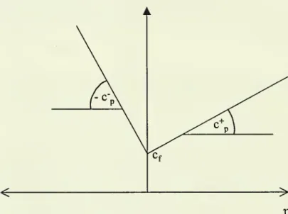
which afixed cost is the simplest. Let C{rj,

K*)

denotethe cost ofadjusting the capital stock by K*ri:

C(r,,K-)

=

_{it.K^m-[^l^_f^}

llll

(8)

where

the

K*

term

ensures that the relative importance ofadjustment costs

remains

unchanged

overtime.^^ Figure3.1 illustratesan exampleofC(.,

)/K*.

^^Thisgoalwould alsobeaccomplishedby K,but

K*

yieldsslighltysimpler

mathemat-ical expressions at a low cost interras ofsubstantive issues.

Also, Ihave allowed proportional costs to differwith respect toupward and downward

adjustraents inorder to talklater aboutthe irreversible investmentcase; for thispurpose, Icouldhave doneit equally wellthrough asymmetricfixedcosts. Allowingfor bothforms

ofasymmetries simultaneoulsy is atrivial but uninteresting extension.

Figure

3.1

Adjustment

Costs

i

The

problem of the firm can be characterized in terms of

two

functions of

Z

and

K*:

V{Z,K*)

and

V{Z,K*).

The

function

V{Z,K*)

represents

the value of a firm with imbalance

Z

and

desired capital

K*

if it does not

adjiost in this period,

and

V{Z,

K*)

is the value ofthe firm which can choose

whether or not to adjust. Thus,

V{Zt,

Kl)

=

U{Zt,

K:)At

+

(1

-

rAt)Et [k(Z,^a.,

K^^m)]

, (9)

and:

V{Zt,K:)

=

ma^!^V{Zt,K:),max{V{Z,

+

ri,K:)-C{rj,K:)}y

(10)

The

nature of the solution of this problem is

now

intuitive. Given the

function

V{Z,K*),

equation (10) provides

most

of

what

is needed to

charac-terize the solution. First, since

C

is positive even for small adjustments, it is

apparent that

when

Z

is near that value for which

V{Z,K*)

is maximized,

the first term

on

the right

hand

side of (10) is larger than the second term; that is, thereis arange ofinaction. Second, sinceboth adjustment costs

and

the profit function are

homogeneous

ofdegreeone with respect to

K*

, so are

V

and

V. Thus, it is possible to fully characterize the solution in the space

of imbalances, Z.

Among

other things, this implies that the range of inac-tion described before, is fixed in the space of Z. Let

L

denote the

minimum

value of

Z

for which there is no investment,

and

U

the

maximum

value for

which there is no disinvestment; thus the range ofinaction is (L, U). Third,

conditional on adjustment, changes

must

not only be large

enough

tojustify incurring the fixed cost, but also the (invariant) target points

must

satisfy:

vz{i)

=

c; (11)

and

Vz{u)

=

-c;, (12)

where Vz

is the derivative of

V

with respect to Z, while I

and

u

denote

the target points from the left

and

right of the inaction range, respectively.

These

first order conditions are

known

as "smooth pasting conditions,"

and

simplysay that, conditional

on

adjustment taking place, it

must

cease

when

the value of an extra unit of investment (or disinvestment) is equal to the additional cost incurred

by

that action.

There are two additional

smooth

pasting conditions:

Vz{L)

=

₄

(13)

and

Vz{U)

=

-c;, ₍₁₄₎

whichensure no expected advantage from delayingor advancing adjustment by one

Ai

around the trigger points.

These

smooth

pastingconditions areenoughtofindthe optimal (L,l,u,U)

rule, given the value function. In order to find the latter, however,

we

need

to go back to equation (9). Standard steps reduce this equation, in the

in-terior ofthe inaction range, to a second order differential equation.

The

two

boundary

conditions required to find

V

are obtained from equalizing thetwo terms

on

the right

hand

side of (10):

V{L,

K*)

=

V{1,

K*)

-

[cf

+

c;{l

-

L))

K\

(15)

and

V{U,

K*)

=

V{u,

K*)

-

(cf

+

c;{U

-

u))

K\

(16)

which simply say that since the investment rule (optimal or not!) dictates

that once a trigger point is reached, adjustment

must

occur at once, the only diff'erence in the value ofbeing at trigger and target points

must

bethe

adjustment cost of

moving

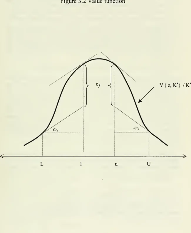
from the former to the latter.

Figure 3.2 illustrates the value function.

Smooth

pasting says that the tangents at

L

and

I have slope c^, while those at

U

and

u

have slope —c~.

Value matching says that the value fimction evaluated at the target minus

the value function evaluated at the trigger point is equal to the variable cost

paid at adjustment plus the fixed cost (all these normalized by

K*

in the

figure).

There are a few particular cases which are worth highlighting because

they appear often in the literature:

1. Ifthere is no variable cost ofinvestment, oncethe adjustment decision

has been talcen, adjustment firomboth sides is complete sincethe

mar-ginal cost of adjustment is zero. Thus, the (L,Z,u,U) rule reduces to

an (L,c,U) rule, where c is the

common

target for investment as well as disinvestment,

and

is that value which maximizes

V{Z,K*)

for any

^"Notethat ingeneral

c^l.

That is, the optimaldynamictarget isgenerally different

fromthe static one.

Figure

3.2

Value

function

*\ /T.r*

V

(z,K') /

K

2. If there are variable costs but no fixed cost, there is no reason for

adjustment to be lumpy, for there are no increasing returns in the

adjustment technology.^^

Once

the boundaries of the inaction range,

L

and

[/, are reached, the firm adjusts just

enough

to avoid crossing outside the inaction range; that is

L

and

U

become

reflecting barriers.

3. Ifthere is a large (not necessarily infinite) cost to disinvestment, then

investment becomes irreversible. In the absence of investment costs,

the investment rule reduces to a single reflecting barrier L, which is to

the left ofone (reluctance to invest). This is the standard irreversible

investment case.

3.1.3

A

detour:

Q-Theory and

Infrequent

Investment.

One

ofthe

main

manifestationsoftheempiricalfailureofpreviousinvestment

theories, has been the difficultyinfinding either a significant

and

sizablerole for g, or evidence that it is a sufficient statistic for investment.

Do

the theories studied in this section help explain these empirical

fail-ures? I see two reasons to believe so.

The

first one is rather negative.

Q-theory is no longer robust in our setting, so there are

many

scenarios where

we

should not expect it to work.

The

second one is

more

positive. In the

subclass of models where it does work, the functional form relating q and

investment is likely to be highly non-linear, thus quite different from the

standard linear regressions leading to the rejection of Q-theory.

On

the fragility ofmarginal q.

It is apparent from the lack of global concavity ofthe value function in figure 3.2, that traditional g-theory is not likely to

work

in the presence of

jumps. Caballero

and Leahy

(1996) develop the argument in detail, which I

summarize

below.

The

value ofthe firm is equal to

K

-\-V^ thus marginal q is:^^

g^(Z)

=

H-V^^

=

l

+

^.

(17)

^^And we have already assumed that shocks are "small" in any given At.

^^Recall that

V

was defined as thepresent value ofprofits net ofadjustment costs and

interest payments on capital.

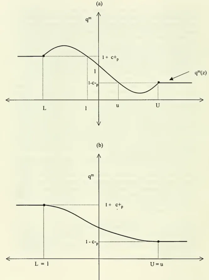
Figure 3.3a plots

g^

against the imbalance measure

Z?^

Smooth

pasting

implies that

q^

must

be the

same

at trigger

and

target points (because

Vz

must

be the

same

at trigger

and

target points); ifthere arejumps, these are points very far apart in state space.

Two

points with the

same

value of

q^

lead to very different levels ofinvestment (zero

and

large). Moreover, since

the value function

becomes

linear outside the inaction range, all points out-side the inaction range (on the

same

side) have the

same

g^,

and

allof

them

lead to different levels ofinvestment. It is apparent, therefore, that the func-tion

mapping

q^

into investment no longer exists. Worse, in between trigger

and

target points, the relationbetween

q^

and

Z

is not even monotonic.

What

is happening? Marginal q is the expected present value of the

marginal profitability of capital. Far from an adjustment point, it behaves as usual with respect to the state of the firm: if conditions improve, future

marginalprofitabilityof capitalrises,

and

so does

q^

. Closetothe investment

point,

on

the other hand, the eff'ect of a change in the state ofthe firm over theprobability ofalarge

amount

ofinvestment inthe near futuredominates.

An

abrupt increase in the stock of capital brings about an abrupt decline in

the marginal profitability of capital as long as the profit function is concave with respect to capital.^^ Thus, an

improvement

in the state of the firm

malces it very likely that it invests in the near future, reducing the expected marginal profitability of capital in the near future, thus lowering the value

of

an

extra unit of installed capital.

Caballero

and

Leahy

(1996)

show

that addingaconvex adjustmentcostto

the problem does not change the basic intuition ofthe

mechanism

described

above.

They

also show,

somewhat

paradoxically, that average _5, which is

often thought of as a convenient albeit inappropriate proxy for marginal _g,

tiirns out to be a

good

predictor ofinvestment even in the presence of fixed costs, although it is no longer a sufficient statistic, except for very special

assumptions about the stochastic nature ofdriving forces.

When

does Q-theory work?

The

failure of g-theory described above is rooted in the presence of

in-creasing returns in the adjustment cost function (8). This featm-e of the

adjustment technology is responsible for the loss of global concavity of the

^"'See,forexample,Dbcit (1993) foracharacterization ofthe (L,Z,u,U)solutioninterms

ofasimilar diagram. ^^_Which

I taketo bethe standardcase.

Figure

3.3

_{Marginal q}

q'"(z)

value function, which is behind the non-monotonicity ofmarginal q?^

Monotonicity of

q^

insidetheinactionrange isrecoveredby dropping the

fixed cost from (8), as

was

donein cases 2

and

3 in section 3.1.2. Figure 3.3b

portrays this scenario. Adjustment at the trigger points no longer involves large projects, thus proximity to these triggers no longer signal the sharp

changes in futiire marginal profitability of capital which were responsible for

the "anomalous" behavior ofq^'^}^ There is still the issue that in the (very) rare event that a firm finds itself outside the inaction range it will adjust

immediately to the trigger, at a constant marginal cost, so different levels of

investment are consistent withthe

same

value ofq^. This is easily remedied by adding a convex

component

to the adjustment cost function:^^

C{r],K*)

=

{AKj^O}K*{cp\T]\

₊

_Cg\vf} /?

>

1. ₍₁₈₎

This is essentially

what

Abel and Eberly (1994) do.^^ Absent the advantage

oflumping adjustment brought aboutbythepresence offixed costs, standard

g-theory is recovered whenever the firm invests. Provided adjustment takes

place, the firmequalizes themarginal benefit ofadjustment

and

the marginal

cost of investing, which is

now

an increasing function ofadjustment:

q''

=

_l

₊

_sgn{rj){cp

₊

Pc,\rjf-'),

for T] y^ 0.

By

setting r] to zero,

we

can obtain the boundaries of inaction in

g''^-space. Indeed, investment will not occur if

1

-

Cp

< q^ <

1

+

Cp.

Abel

and

Eberly (1994) go further, and

show

that their insight is robust

to the presence of/Zou;-fixed costs.

That

is, fixed costs which are multiplied

by

At; ifadjiistment occured instantaneoulsy, the firm effectively

would

pay nofixed cost. Because oftheconvex adjustment component, thefirm chooses not to adjust instantaneously

and

pays the fixed costs instead. In a sense,

^^Indeed, value functions for (5,s) models are often only i<'-concave.

^^Ofcourse, once at the trigger, large projects may result from the accumulated and

—

more or less

—

continuous response to a sequence of shocks with the same sign. But this does not give rise to a sharp change in profitability since investment occurs only in

response and tooffset new, as opposed toaccumulated, changes inprofitabihty. ^'^Which, atthe same time, makes transitions intothe inactionrange lessrare.

^*Needless to say, it is trivial to add asymmtries to the adjustmentcost function. But

that is beside the point ofthis section.

the endogenous adjustment decisions

and

the fact that the fixed cost goes

to zero as adjustment speeds up, ensures that the fixed cost remains rela-tively "small,"

and

so do investment projects.^^ _{It is important to realize}

that their paper "unifies" ^'-theory with irreversible investment

and

regula-tion (i.e. infrequentbut infinitesimal adjustments) problems, but it does not unify it with the standard (5, s) hterature on

lumpy

adjustment, which is, unfortunately, the

way

many

have interpreted their results.

Barnett

and

Sakellaris (1995) study a panel of U.S. firms searching for

evidence on a reduced sensitivity of investment to changes in q

when

the

latter is close to one (the "inaction" range).

They

find theopposite; in their panel, afirm's investment seems to be

more

rather than less responsive to _q

when

q is closeto one. Abel and Eberly (1996), however,

show

that allowing

for unobservedheterogeneityintheinactionrangerelevant fordifferenttypes

of investments could explain the negative Barnett-Sakellaris finding.

Taking stock.

One

may

be inclinedtoconclude fromthissectionthat beforegoingahead with g-theory one should check whether investment literally exhibits

jumps

or not. This is not the lessonI draw, however.

For once, this is not right. It is not difficult to

add

a time to build mech-anism such that a

lumpy

project is

decomposed

into a fairly

smooth

flow,

without alteringthe argument of

why

marginal qfails inthe presenceof fixed costs.

But

more

importantly, I suspect the

main

lesson is one of modesty. I

doubt that researchers will often find the required data and/or patience to

determine whether onescenario or the other holds. Inthis case,

we

might as well acknowledge that therelationship between marginal q

and

investment is

not robust,

and

that average_qis unlikely tobe asufficientstatistic for

invest-ment.

Of

course it is important to include variables that captureknowledge

of the future

on

the right

hand

side ofinvestment equations, but

we

should avoid reading "too

much"

from these regressions.

^^Alternatively, if one assumes perfect competition and constant returns to scale, the

profit function becomes linear with respect to capital (ifthe other factors ofproduction canbeadjustedat will),sochangesininvestmentdo notfeed backinto q. Inthis extreme

case, the modified (i.e. with an inaction range) g-theoryworks well even inthe presence

of traditional fixedcosts.

3.1.4

Another

detour: SeveraJ

misconceptions

about

irreversible

investment.

As

I mentioned before,

when

describing the special case of irreversible

in-vestment, the regulation barrier, L, is to the left of one.

That

is, investment

occurs only

when

the stock of capital is substantially below the frictionless

stock of capital. Alternatively, investment occurs

when

the marginal prof-itability of capital is substantially above the cost of capital. This is the

famous

"reluctance to invest" result.

There are several misconceptions about the implications of this

"reluc-tance" result. I will mention three of them. It is often said that, (a)

re-luctance implies that, in the presence ofirreversibility, the firm accumulates

less capital; (6) since reluctance rises with uncertainty (the regulation point

moves

further to theleft),

more

uncertaintyimplies less capital;

and

(c)

stan-dard present value techniques are inappropriate because reluctance reflects

the value of the "option to wait" for

more

information before irreversibly

sinking resources

and

this is not taken into account by the standard

formu-lae.

In orderto

show

the fallacious nature ofthe first statement, it is useful to

go back to our canonical problem

and

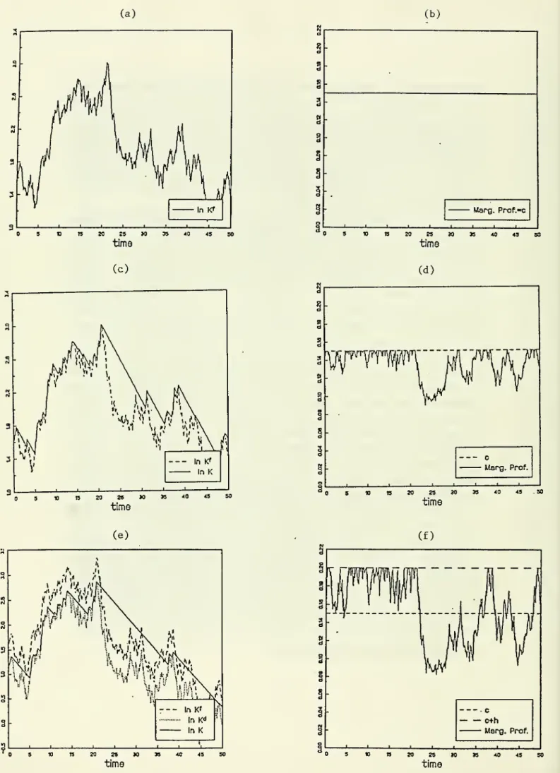
simulate the path ofthe (log of) stock

of capital of a firm facing no irreversibility constraint. Panel (a) in figure 3.4 does so for a

random

realization ofthe path of 6. Panel (b) in the figure

shows the corresponding path ofthe marginal profitability of capital, which

is equal to the constant

—

frictionless

—

cost of capital, r.^'^

Imagine

now

imposing an irreversibility constraint

on

the firm, but

as-sume

that the firm does not modify its "frictionless" investment rule

when-ever it can invest. This is portrayed in panel (c) of the figure.

The

solid

and

dashed lines represent the actual

and

frictionless stocks of capital,

re-spectively. It is apparent that the firm would, on average, have too

much

capital, for it

would

have the

same

stock of capital in

good

times, but too

much

in

bad

times.

The

counterpart ofthis is in panel (d), which shows that

on

average the marginal profitability of capital is below the cost of capital.

Reluctance to invest in

good

times is an optimal response attempting to offset the natural tendency to over-accumulate capital induced

by

the

irreversibility constraint. Panel (e) illustrates this point.

The

solid

and

dashed lines represent the

same

variables as in panel (c), while the dotted

fine illustrates the target stock of capital

when

the firm behaves optimally.

'"These figures axe from Caballero (1993a).

Figure 3.4:

Reluctance

and

Its

Counterpart

(a) (b) -1 1 1 1 r time time (c) (d) 40 4S SO time time (e) 40 43 so time time

The

counterpart ofthe negativevalue of ln{K'^/K^) is a positive constant h

in the marginal profitability of capital required for investment to take place

(panel f). Itis apparent thatwhether the stockof capitalis onaverage higher or lower than without the irreversibility constraint is unclear; the firm has too little capital during

good

times but too

much

during very

bad

times.

A

precise answer depends onthings about which

we

know

little,

and

which

may

turn out to yield only second order effects.'^^

It is

now

easy to see the fallacious nature ofthe second statement.

More

uncertainty raises reluctance precisely because it raises the need to reduce

the extent of excessive capital during the

now

deeper recessions.

Without

raising reluctance, an increase in uncertainty would raise the average stock

of capital in the presence of irreversibility constraints. This occurs because

there

would

now

be greater capital accumulation during extremely

good

times which

would

not be offset by large disinvestment during extremely

bad

times.^^

The

third misunderstanding is of a different nature. In

my

view, it is

the result of insightful but, unfortunately, abused language. First,

what

is right: there is nothing mysterious about irreversibility constraints as a

mathematical problem.

Dynamic

programing works, in the

same

way

it does

with other,

more

traditional, adjustment frictions. This

means

that present value formulae, using the correct calculation offuture marginal profitability of capitalalsowork.

Of

coursesuch calculations

must

be performed along the optimal investment path, constraints included!

What

is wrong: thestandard analysis

must

be modified to consider the value ofthe "option to wait."

As we

have seen, there is no need to do so. However, one

may

choose to follow an alternative path, in which one starts by evaluatingthe future

mar-ginal profitability of capital without considering the effect offuture optimal investment decisions

on

marginal profitability. This "mistake" can then be

^^See Bertola (1992), Caballero (1993a), Bertolaand Caballero (1994) for early discus-sions ofthis issueand oftherelateduncertainty-investment misconception. Morerecently,

Abel and Eberly (1996b) have formalized theseclaims and made them moreprecise. ''^This does not mean that one cannot construct scenarios where an increase in

uncer-tainty reduces investment. For example, if there is an increase in perceived future

un-certainty, the investment threshold may jump today

—

i.e., before the variance ofshocks does

—

resulting inan unambiguous decline in investment.

Also, oneshould not confuse changes in uncertaintywith changes in the probability of

abadevent. Thelatter linksincreases inuncertaintyto a reduction inexpectedvalue, an

entirely different and more straightforward effect on investment. One can find traces of this confusionin the (informal) credibility literature.

"corrected" with a term that has an option representation. This alternative

way

of doing things is akin to the arbitrage approach in finance,

and

it

was

nicely portrayed in Pindyck (1988).

The

confusion arises, in

my

view, from mixingthe language in the two approaches.^'^

A

related claim exists for a once and for all project (as opposed to

incre-mental investment). It issaid that thesimple positive net present value rule

used in business schools to decide whether a project should be implemented

does not hold because it does not consider the option to wait

and

decide

tomorrow,

when

more

information is available. Since I have never taught at

abusiness school I cannot argue directly against that claim. However, ifthe issue is whether to invest today or tomorrow, the right criterion has never

been invest if

NPV

is positive

—

at least that is

what

we

teach economics

undergraduates. This is a case ofmutually exclusive projects, thus the right criterion has always been to

compare

their net present value and take that

with the highest

NPV,

provided it is positive. If investment is irreversible,

the project invest tomorrow has a lower

bound

at zero (because investment

will not occur if

NPV

looks negative tomorrow), which the project invest

today does not. Thus, other things equal, irreversibility necessarily

makes

investing

tomorrow

more

attractive than investing today.

3.1.5

Adjustment

hazard

At

a qualitative level, the {L,l,u,U) models described above capture well

the nonlinear nature of microeconomic adjustment. Maintenance

expendi-tures aside, investment is mostly sporadic

and

oftenlumpy; scarcelyreacting

to small changes in the environment but abruptly undoing accumulated

im-balances

when

they

become

sufficiently large, and with possibly significant

asymmetries between investment

and

disinvestment.

At

an empirical level, however, these characterizations aretoo stark. For

reasons,

some

of which

we

vmderstand

and

most of which

we

do not, firms

respond differently to similar imbalances'over time

and

across firms.

Ca-ballero

and

Engel (1994) propose a probabilistic instead of a deterministic

adjustment rule. Rather than having aclear demarcationbetween regions of

adjustment

and

inaction, they

model

a situation where large imbalances are ^^See Bertola (1988) for one of the first discussions of this issue in the economics

lit-erature. There is also a related discussion in applied mathematics; see, for example, El Karoui andKaratzas (1991). Abel etal. (1996) haverecently revisited andexpanded the

discussionon the relationbetweenthe two approaches.

more

likely to trigger adjustment than small ones."''*

There are

many

formal motivations for such an assumption.

A

particu-larly simple one, pursued by Caballero

and

Engel (1994), is to

assume

that

Cf in the adjustment cost function (8) is an i.i.d.

random

variable, both

across firms

and

time. Althoughtechnically

more

complex, the nature ofthe

problem is not too different from that of the simpler (L,/,u, U) model. Let

uj denote the

random

fixed cost,

and

G{ijj) its time invariant distribution. It is possible to characterize the problem ofthe firm in terms of

two

functions

similar to those used before:

V{Z,

K*) and V{Z,

K*,uj), the value of a firm

with imbalance Z, desired capital K*,

and

realization of fixed adjustment

cost u). In particular,

V{Z,

K*)

is the value ofthe firm provided it does not adjust, while

V{Z,

K*

,u) is the value ofthe firm

when

itis left freeto choose

whether or not to adjust. Thus,

V{Zt,

Kl)

=

U{Zt,

K:)At

+

(1

-

rAi)E, [^(Z,+At, i^;+A„u;t+At,)] , (19)

V{Zt,K:,u)=m8.x{v{Zt,K;),ma.x{V{Z,

+

T^,K:)-C{ri,K;,c,t)}]. (20)

Not

surprisingly, the nature ofthe solution is not too different from that

of the {L,l,u,U) case. Indeed, conditional

on

u

it is an {L,l,u,U) rule,

although there are additional intertemporal considerations, since the firm

weighs the likelihood of drawing higher or lower adjustment costs in the

future.

Without

conditioning on cu, it is a probabilistic rule in the space of

imbalances.

In order to simplifythe exposition, I will suppress the proportional costs.

Thus, conditional on adjustment, the target point is the

same

regardless of whether the firm is adding or substracting to its stock of capital (i.e.

I

=

u

=

c). Moreover, let

me

define a

new

imbalance index centered around

zero:

a;

=

ln(Z/c).

The

probability ofadjustmentriseswiththe absolute value ofx becausethere

are

more

realizations of adjustment costs whichjustify adjustment. This is

the sense in which the {S,s) natiire ofthe simpler models is preserved. Let

^^_{Another advantage ofthis approach}

is that it nests linear models as the probability ofadjustment becomes independent ofZ.

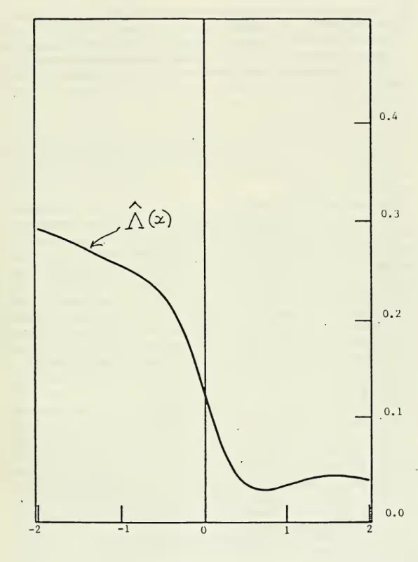
A(a;) denote the function describing the probabihty of adjustment given x,

and

call it the adjustment hazard function (see Caballero

and

Engel(1994)).

Given an imbalance x, it is no longer possible to say with certainty

whether or not the firm will adjust, but the expected investment by the firm is given by:

E

Ilit/Ku\x]

=

(e-^

-

l) A{x)

«

-xA{x), (21)

whichissimply theproductoftheadjustment if itoccurs,

and

theprobability

that adjustment occurs."^'* Aggregation is

now

only a step away.

3.2

Aggregation

Unlike microeconomic data, aggregate investment series look fairly smooth. Large microeconomic adjustments are far from being perfectly synchronized.

The

question arises, and this was the maintained hypothesis during the 80s, as to whether aggregation eliminates all traces of

lumpy

microeconomic

ad-justment.

The

answer is a clear no.

Doms

and Dunne's evidence

on

the role ofsynchronization ofprimaryspikes in accounting for aggregate investment,

and

on the high time series correlation between aggregate investment

and

a Herfindahlindexofmicroeconomicinvestments, aswellasthe

more

structural empirical evidencereviewed in the next section, support this conclusion.

With

the setup at hand, aggregation proceeds in two easy steps.

To

simplify things further, I will define the aggregate as the behavior of the

average, rather than the weighted average."^^

Both

steps rely on having a large

number

ofestablishments, so that laws

of large

numbers

can be applied. In the first step, one takes as the average investment rate (i.e. theratioofinvestmenttocapital) ofestablishmentswith

more

or less the

same

imbalance ofcapital, x, the conditional expectation of this ratio given in equation (21):

ih/KtY

=

-xA{x), (22)

where

the superscript x denotes the aggregate for plants with imbalance x. ^^_{Caballeroand Engel (1994)refertoA(a;) as the "effectivehazard" to capture the idea} that,through a normalization,it alsocaptures scenarioswhereadjustment, ifitoccurs, is

only afraction oftheimbalance x.

^^Using microeconomic data, Caballero, Engel and Haltiwanger (1995) show that in

U.S. manufacturing this approximationis. See the (1997) version ofCaballero and Engel

(1994) for adetailed discussion of the issue.

The

second step just requires averaging across all x. Let f{x,t) denote

the cross sectional density of establishments' capital imbalances just before

investment takes place at timet.

Then

the aggregate investment rate at time

t, {It/Kt^, is:

{It/Ktf

=

-

_y

xA{x)f{x,t)dx. (23)

This is an interesting equation, with

macroeconomic

data on the left

and

microeconomic data on the right

hand

side.

An

example serves to illustrate this aspect ofthe investment equation: Ifthe adjustmenthazard is quadratic

K{x)

=

Ao

+

Xix

+

\2X^,

equation (23) reduces to:

ih/K,)^

=

-AoXf

'

-

AiXP

- A2Xf

_{\ (24)}

where Xt \Xt

and

X}

denote, respectively, the first, second

and

third

moments

ofthe distribution ofestablishments' imbalances.

IfAi

=

A2

=

0, the

model

only has aggregate variables, both

on

the right

and

left

hand

side. Indeed this case corresponds to the celebrated partial

adjustment model,

and

it also coincides with the equation obtained from a

quadratic adjustment cost

model

with a representative agent (e.g.

Rotem-berg (1987)

and

Caballero

and

Engel(1994)). If either Ai or A2 is different

fromzero, however, information about the cross sectional distribution of

im-balances is needed

on

the right

hand

side. All the microeconomic models

discussed in this section yield situations where higher

moments

ofthe cross sectional distribution play a role.

3.3

Empirical

Evidence

There

are

two

polarempirical strategies usedto estimate (23), with a

contin-uum

ofpossibilities in between.

At

one extreme, one can use microeconomic data to construct all the elements

on

the right

hand

side; in particular one canconstructthe pathofthecross sectional distribution

and

estimatethe

ad-justment hazard as an accounting identity, or estimate a parametric version of it.

At

the other extreme, one can attempt to learn about the adjustment hazard from aggregate data only, by putting

enough

structure

on

the sto-chastic processes faced by firms and

by

starting with a guess on the initial

cross sectional distribution.

Both

avenues have been explored, with similar results along dimensions they can be compared.