HAL Id: hal-02972284
https://hal.inrae.fr/hal-02972284
Submitted on 20 Oct 2020
HAL is a multi-disciplinary open access
archive for the deposit and dissemination of
sci-entific research documents, whether they are
pub-lished or not. The documents may come from
teaching and research institutions in France or
abroad, or from public or private research centers.
L’archive ouverte pluridisciplinaire HAL, est
destinée au dépôt et à la diffusion de documents
scientifiques de niveau recherche, publiés ou non,
émanant des établissements d’enseignement et de
recherche français ou étrangers, des laboratoires
publics ou privés.
Distributed under a Creative Commons Attribution| 4.0 International License
Scanning (ALS) data
Jean-Romain Roussel, David Auty, Nicholas Coops, Piotr Tompalski, Tristan
R.H. Goodbody, Andrew Sánchez Meador, Jean-François Bourdon, Florian de
Boissieu, Alexis Achim
To cite this version:
Jean-Romain Roussel, David Auty, Nicholas Coops, Piotr Tompalski, Tristan R.H. Goodbody, et
al.. lidR: An R package for analysis of Airborne Laser Scanning (ALS) data. Remote Sensing of
Environment, Elsevier, 2020, 251, pp.112061. �10.1016/j.rse.2020.112061�. �hal-02972284�
Contents lists available at ScienceDirect
Remote Sensing of Environment
journal homepage: www.elsevier.com/locate/rse
Review
lidR: An R package for analysis of Airborne Laser Scanning (ALS) data
Jean-Romain Roussel
a,⁎, David Auty
b, Nicholas C. Coops
c, Piotr Tompalski
c,
Tristan R.H. Goodbody
c, Andrew Sánchez Meador
b, Jean-François Bourdon
d, Florian de Boissieu
e,
Alexis Achim
aa Centre de recherche sur les matériaux renouvelables, Département des sciences du bois et de la forêt, Université Laval, Québec, QC G1V 0A6, Canada b School of Forestry, Northern Arizona University, United States of America
c Faculty of Forestry, University of British Columbia, 2424 Main Mall, Vancouver, BC V6T 1Z4, Canada
d Direction des inventaires forestiers, Ministère des Forêts, de la Faune et des Parcs du Québec, QC G1H 6R1, Canada e UMR TETIS, INRAE, AgroParisTech, CIRAD, CNRS, Université Montpellier, Montpellier, France
A R T I C L E I N F O
Keywords:
LiDAR lidR R
Airborne laser scanning (ALS) Software
Forestry
A B S T R A C T
Airborne laser scanning (ALS) is a remote sensing technology known for its applicability in natural resources management. By quantifying the three-dimensional structure of vegetation and underlying terrain using laser technology, ALS has been used extensively for enhancing geospatial knowledge in the fields of forestry and ecology. Structural descriptions of vegetation provide a means of estimating a range of ecologically pertinent attributes, such as height, volume, and above-ground biomass. The efficient processing of large, often technically complex datasets requires dedicated algorithms and software. The continued promise of ALS as a tool for im-proving ecological understanding is often dependent on user-created tools, methods, and approaches. Due to the proliferation of ALS among academic, governmental, and private-sector communities, paired with requirements to address a growing demand for open and accessible data, the ALS community is recognising the importance of free and open-source software (FOSS) and the importance of user-defined workflows. Herein, we describe the philosophy behind the development of the lidR package. Implemented in the R environment with a C/C++ backend, lidR is free, open-source and cross-platform software created to enable simple and creative processing workflows for forestry and ecology communities using ALS data. We review current algorithms used by the research community, and in doing so raise awareness of current successes and challenges associated with parameterisation and common implementation approaches. Through a detailed description of the package, we address the key considerations and the design philosophy that enables users to implement user-defined tools. We also discuss algorithm choices that make the package representative of the ‘state-of-the-art’ and we highlight some internal limitations through examples of processing time discrepancies. We conclude that the development of applications like lidR are of fundamental importance for developing transparent, flexible and open ALS tools to ensure not only reproducible workflows, but also to offer researchers the creative space required for the progress and development of the discipline.
1. Introduction
1.1. Airborne Laser Scanning (ALS)
Airborne laser scanning (ALS), also known as LiDAR (Light Detection and Ranging) technology has revolutionised data acquisition and resource quantification in natural sciences and engineering. ALS is an active remote sensing technology, that uses laser pulses to measure the time, and intensity, of backscatter from three-dimensional targets on the Earth's surface (Wulder et al., 2008). Retrieval of the position of
the targets is made possible using precise geolocation information from Global Navigation Satellite Systems (GNSS), and orientation data from an Inertial Measurement Unit (IMU). When combined, the positional accuracy of the derived ALS data sets provide sub-meter measurement accuracy of surfaces, providing best-available data describing the three- dimensional structure of landscapes. As a result, ALS has been widely used for the generation of bare Earth terrain models (Furze et al., 2017), which have wide applicability in land surveying, hydrological studies and urban planning (e.g. Chen et al., 2009; Yu et al., 2010). In addition, high positional accuracy of returned point clouds and the ability of laser
https://doi.org/10.1016/j.rse.2020.112061
Received 29 February 2020; Received in revised form 19 August 2020; Accepted 30 August 2020
⁎Corresponding author.
jean-romain.roussel.1@ulaval.ca (J.-R. Roussel).
0034-4257/ © 2020 The Author(s). Published by Elsevier Inc. This is an open access article under the CC BY license (http://creativecommons.org/licenses/BY/4.0/).
pulses to pass through small openings in forest canopies facilitate the direct measurement of a number of key forest attributes such as tree height or canopy cover. Laser energy returned to the sensor can be recorded as either a series of discrete xyz locations (the most common data storage format), or a fully digitised return waveform (Mallet and Bretar, 2009). To date, the majority of ALS providers globally provide data in discrete return format largely due to established processing streams. Development of methods for processing full waveform data are ongoing and not yet considered to be conventional practice.
In forestry, two well-established methods have been developed for deriving forest attributes: individual tree segmentation (ITS) and the area-based approach (ABA). ITS allow both individual tree tops to be located, and tree crowns delineated (Hyyppä and Inkinen, 1999; Jakubowski et al., 2013), followed by derivation of individual tree at-tributes within each delineated crown. This method depends on the accuracy of tree identification and can be prone to errors that result from over- or under-estimation of tree crown dimensions (White et al., 2016). In ABA, attributes are estimated for pre-established grid-cells based on metrics that summarise the distribution of the point cloud within each cell (Næsset and Økland, 2002; White et al., 2013). The grid cell is therefore a fundamental unit of the ABA, offering more spatial detail when compared to a traditional polygon-based inventory. For example, attributes that have been successfully modelled using ALS data over various forest types globally include canopy height, canopy cover, stand basal area, biomass, and volume estimates Maltamo et al. (2014); White et al. (2016). In addition to these two methods to mea-sure characteristics of the forest resource, ALS can be used for a wide variety of usages including mapping water bodies (e.g. Morsy, 2017; Demir et al., 2019), forest roads mapping (e.g. Ferraz et al., 2016; Prendes et al., 2019), fire fuel hazard (Price and Gordon, 2016) or wildlife habitat assessment (e.g. Graf et al., 2009; Martinuzzi et al., 2009).
1.2. Historical software development for ALS processing
The widespread interest and adoption of ALS-based technologies in the forestry arena over the past decade have generated a need for vi-sualisation and processing software and scripts. Forest inventory data are often stored within geodatabases linked to aerial photographic in-terpretation (API) information represented by polygonal topology. As a result, many forest industry professionals and managers are accustomed to a vector-based analysis framework for data manipulation and ana-lysis. The advent of ALS-based datasets in the early 2000s facilitated the need for software solutions to display and analyse three dimensional point cloud data. Initially, software solutions were developed in-house, by university research groups or data providers, with more professional solutions following as the user market grew. Built from the
photogrammetry disciplines, Terrascan (Soininen, 2016) was one of the first surveying-based software platforms to be able to input and process ALS-derived 3D point clouds. The program specialised in the classifi-cation of point clouds into ground and non-ground returns, allowing generation of terrain models, a fundamental feature of the software. One of the first forestry-specific ALS data analysis platforms was FU-SION (McGaughey, 2015), originally developed by the University of Washington and the US Forest Service (USFS) and released in the early 2000s. The software, pioneering at the time, was one of the first packages specifically designed for the forestry research community, and was one of the first platforms where ITS was available. Its capabilities include extraction of 3D point clouds over forest inventory plots, point cloud visualisation, and calculation of plot and landscape-level metrics. FUSION also allows integrated large-scale batch processing of ALS da-tasets, allowing for simple computation of wall-to-wall metrics, which at the time was cumbersome and could not be easily completed in commercial GIS or image processing environments without extensive pre-processing.
As the user-base of ALS forestry applications grew, so did the re-quirements for software solutions. A number of commercial companies started to develop ALS-specific software. Today, many GIS and image processing tools have graphical user interfaces and the ability to process ALS data with add-ons available for ESRI software, Whitebox, and image processing stand-alone software such as ENVI.
A number of open source tools exist that allow users to capitalise on the complexity of ALS datasets. CloudCompare is an example of a commonly used open source software suite that allows ALS data to be analysed, manipulated, and merged. Among commercial software packages, LAStools is also commonly used for various large-scale ALS processing tasks. LAStools has been specifically designed for processing ALS data, from plots to large landscapes, and is free to use on small datasets, while commercial solutions unlock advanced capabilities for in-depth processing and broad area implementation. A number of modules available within LAStools are open source, including the compressed LAZ format that reduces storage size of original un-compressed files (Isenburg, 2013). Table 1 shows a selected set of active free and open source software currently capable of processing LiDAR point clouds and that include useful tools for forestry and ecology ap-plications.
1.3. The move towards free and open-source software
The current software landscape for ALS data processing, in parti-cular for forestry applications, contains a mix of solutions. In some cases, tools are open-source and cross-platform (e.g. PDAL). In other cases, software are free to use, but the source code itself is not publicly available and use is restricted to the Microsoft Windows platform (e.g Table 1
An overview of free and open source ALS processing packages or modules that include tools useful in forestry and ecology contexts.
Package Brief Description Comment
PDAL Point Data Abstraction Library in C/C++. Designed for translating and processing point cloud data.
PDAL Contributors (2018) Generic and multi-purpose C++ library PCL Point Cloud Library in C++. Cross-platform and designed for 2D/3D image and point cloud processing.
Rusu and Cousins (2011)
CloudCompare 3D point cloud and triangular mesh processing software. It was originally designed to perform comparisons between two dense 3D point clouds
LAStools A suite of LiDAR processing tools widely known for their very high speed and high productivity. They combine robust algorithms with efficient I/O and clever memory management to achieve high throughput for datasets containing billions of points.
A few modules for LAS files manipulation are open source and cross-platform
Whitebox GAT GIS capabilities for ALS including basic and advanced tools for ALS processing
FUSION/LDV A collection of task-specific command line programs (FUSION) and a viewer (LDV) McGaughey (2015) Sources available on request only. Not cross- platform.
GRASS GIS FOSS Geographic Information System software suite used for geospatial data management. It supports basic and advanced ALS data processing and analysis.
SPDlib A set of open source software tools for processing laser scanning data (i.e., LiDAR), including data captured from airborne and terrestrial platforms. Bunting et al. (2011, 2013)
FUSION, LAStools). Some solutions propose free and open-source components on multiple platforms, but also contain closed source functionalities (e.g. LAStools). There are also a number of closed- source, single-platform commercial solutions requiring a paid sub-scription or licence.
Common to all closed source solutions is the use of specific algo-rithms or workflows for ALS that are essentially black boxes to the users. For example, it is not possible to know what is used internally to segment ground points in software like TerraScan. While it can be guessed that it is based on the Progressive TIN Densification (PTD) (Axelsson, 2000), this is not documented nor verifiable. Similarly, the LAStools documentation states that “a variation of the PTD” is used without providing further details of the variant. If a closed-source classification routine misclassifies points, it is impossible to glean from the documentation why this happened, and consequently difficult to tune the corresponding settings or improve the method. This example of ground classification also applies to other routines and algorithms, in-cluding tree segmentation, point cloud registration, point cloud classi-fication, etc.
Recently, however, the remote sensing community has shown a growing interest in the open-source and open-data philosophy. The availability of free and open-source software (FOSS) is of fundamental importance because it gives direct insight into the processing methods. In addition to its educational value, such insight allows users to obtain a better understanding of the consequences of their parametrisation. This is particularly important in remote sensing, a field in which complex algorithms are often strongly affected by implementation details. FOSS also serves as a catalyst for innovation as it avoids the need to duplicate programming efforts, and thus facilitates community-led development. Large FOSS projects usually assemble communities of users and pro-grammers that can report, fix or enhance the software in a highly in-teractive and dynamic way. Finally, FOSS are generally free-to-pay and cross-platform, both of which are very important, especially in the academic context.
One example of the rapidly growing adoption of the FOSS philo-sophy is the increasing use of the R environment (R Core Team, 2019) for research in natural sciences (Carrasco et al., 2019; Crespo- Peremarch et al., 2018; Mulverhill et al., 2018; Tompalski et al., 2019b). R is a FOSS and cross platform environment for statistical computing and data visualisation supported by the R Foundation for Statistical Computing. A key feature of R is the ability for users to create package extensions that link to the base R architecture, and to its data storage and manipulation model. Based on this wide uptake of R, along with its FOSS philosophy, we describe an open source and cross-plat-form R library titled lidR (Roussel and Auty, 2020), created not only to perform many of the tasks commonly required to analyse ALS data in forestry, but also to provide a platform sufficiently flexible for users to design original processes that may not necessarily exist in any other software.
1.4. Manuscript organisation and intentions
The lidR package has been rapidly adopted and is now widely used, especially in academic research. It is widely cited internationally (see section 6) and there are now several training courses designed to teach the package that have been created independently of the lidR development team. Consequently, this paper was written to clarify the goals and the design of the package for a broad audience in environ-mental sciences, and to inform the community of our development choices. While the package is comprehensively documented, we have never explicitly set out our motivations underpinning its development because this kind of information does not belong in the user manual. lidR is part of a large suite of available tools that all bear their own strengths and weaknesses. Learning new tools can be laborious, so we believe it worthwhile to clarify what lidR is designed for, to help potential users and developers decide if it will meet their analysis needs
upstream of the learning curve. This paper also serves as a general re-view of the various steps available to the practitioner for processing ALS-based point clouds, with an emphasis on the forestry and ecology contexts. However, our intent was not to provide detailed descriptions of the algorithms hosted in lidR that can be used to perform these steps because these are already documented in detail in peer-reviewed pa-pers, which are all referenced in the text.
In this manuscript we focus on four components of the lidR ap-proach. In the first part (section 2), we focus on the architecture of the package. In the second part (section 3), we focus on key processing algorithms for data acquired from discrete return ALS systems, given their prevalence in the ALS market today, to demonstrate the efforts we have made in the lidR package to provide a wide range of tools from the peer-reviewed literature. We follow a likely conventional ALS workflow involving ground classification and terrain interpolation, height normalisation, construction of digital canopy models, and ex-traction of ALS metrics to allow ABA model development. In the third part (section 4) we highlight the versatility of the lidR package in its fundamental formulation, which allows for a highly flexible program-ming environment to implement less common, or more innovative processing approaches. We provide some specific examples on how this flexibility can be used and leveraged. We conclude (section 5) with general comments on the processing speed and future functionalities of the package.
As lidR is constantly evolving, it is important to state that this manuscript reflects the state of the package in its 3.0 version. While some information might become outdated, such as the supported for-mats (section 2.2), the benchmarks (section 5), or the currently im-plemented algorithms, the overall intentions and design choices will remain valid.
2. lidR: an R package for ALS data processing
2.1. Architecture and design
lidR is a point-cloud oriented R package designed to be integrated into the R spatial analysis ecosystem by supporting inputs/outputs in formats defined by the packages sp (Pebesma and Bivand, 2005; Bivand et al., 2013), sf (Pebesma, 2018) and raster (Hijmans, 2019). It is designed with the FOSS philosophy in mind: the source code is open and freely modifiable, and the development is both driven by feature requests from users and open to third-party modifications/additions, thus allowing the package to constantly evolve.
The lidR package was created to provide a variety of customisable processing strategies with the goal of enabling users to manipulate and analyse their data easily. In addition to a set of internally-defined functions, lidR offers the possibility to implement user-defined func-tions, so that processing can be specialised and tailored to meet in-dividual management and research needs. The package was developed to enable users to try, test and explore methods in a straightforward manner. In other words, it is not only designed as a toolbox, but also as a suite of tools that users can use to build new tools.
To achieve this objective, tools available within lidR can be clas-sified into three categories: (1) generic processes used in forestry, such as ABA processing (section 3.5) or digital terrain modelling (section 3.2), (2) specific algorithms implemented from the peer-reviewed lit-erature, such as snag detection (section 3.7) or tree segmentation methods (section 3.6), and (3) versatile tools providing a way to design new processing methods, such as a new classification routine, a new intensity normalisation routine, or new predictive models (section 4).
The architecture behind lidR relies on two alternative ways to process data. The first (classical) way involves reading a file and loading the point cloud in memory to enable subsequent processing through the application of R functions. This allows the application of built-in functions from the package itself, such as digital terrain/surface model generation, but also any user-defined functions. This first option
is designed to develop and test either existing or user-defined methods on simple test cases. Once this is done, the second option is designed to apply a working routine on a broader area involving too many files to be loaded at once into memory. It consist of creating a link to a di-rectory where a collection of files is located. Using what we call the “LAScatalog processing engine” (section 3), any internal or user-defined function can also be applied over a broad geographic area. The engine allows users to load successive regions of interest (ROI) buffered on-the- fly. This option is akin to batch processing, and the internal engine embeds all the complexity of on-the-fly buffering, parallelism, mapping, merging and error handling to help users focus on the development of their methods rather than being hindered by computing issues. With this architecture, the lidR package offers a straightforward approach to designing innovative processing workflows and scaling them up over broad landscapes.
2.2. ALS data formats supported
Discrete return ALS sensors record three coordinates per point as well as several types of supplementary data for each point. Reading, writing and storing these ALS data is a critical preliminary step before any subsequent analysis. ALS data is most commonly distributed in the LAS open format, which is specifically designed to store LiDAR data that is standardised, and officially and publicly documented and maintained by the American Society for Photogrammetry & Remote Sensing (ASPRS, 2018). LAS format enables point cloud data to be stored using an optimised amount of memory but without being com-pressed. The requirement to store and share ALS data provided impetus for improved data compression (Pradhan et al., 2005; Mongus and Žalik, 2011). Since there is currently no official standard to compress point cloud data files, several different schemes were developed over the last decade to compress LAS files, such as ‘LizardTech LiDAR compressor’ (LizardTech), ‘LAScompression’ (Gemma lab) or ‘zlas’ (ESRI), many of which are proprietary, resulting in difficulties sharing the data between users or platforms. However, since the development of the LASzip library (Isenburg, 2013), the LAZ format has become the
de facto standard, because it is free and open-source and can be
im-plemented and supported by any software.
As a consequence of the open nature of the LAS and LAZ formats, their widespread use in the community and their adequacy with pro-cessing requirements, the lidR package is designed to process LAS and LAZ files both as input and output, taking advantage of the LASlib and LASzip C++ libraries via the rlas package (Roussel and De Boissieu, 2019). Due to the underlying input / output drivers, lidR also supports LAX, or spatial indexing, files (Isenburg, 2012) to increase access speeds when undertaking spatial queries (see section 5). Alternative open formats do exist, such as PLY, HDF5 or E57, but their use is either ill- suited for large ALS coverages or they have not been widely adopted, in the forestry community at least, and are thus not yet supported by lidR.
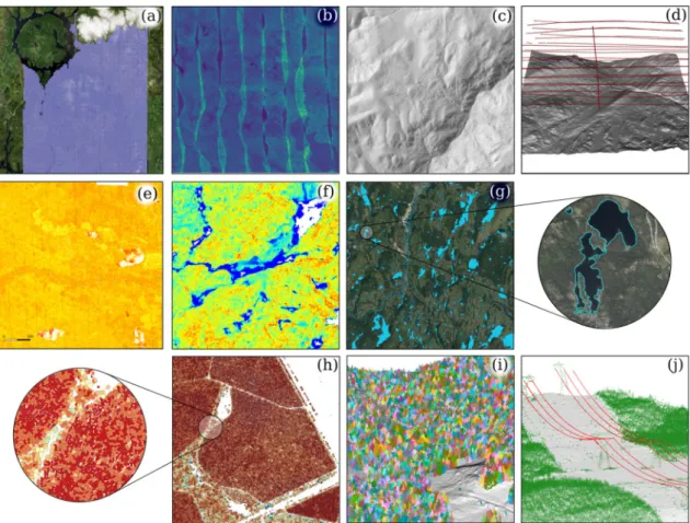
Fig. 1 shows a selected set of outputs and displays that can be generated by the lidR package. Some were produced using built-in, ready-to-use functions and can be easily reproduced from the user- manual examples while others were derived from user-defined func-tions designed on top of the existing versatile tools provided in the package.
3. Common processing workflow in lidR
ALS data processing relies on recurring steps that are systematically applied to a dataset. These steps include ground classification, digital terrain generation, digital surface model generation, height normal-istion of the point cloud and, in the case of forestry applications, an ABA and/or ITS analysis. While, the lidR package was designed pri-marily to explore processing beyond these steps (section 4), it embeds the required tools to apply these routines. All tools dedicated to such
common processing steps are derived from the peer-reviewed literature. As far as possible, lidR aims to provide a wide range of processing options implemented from original papers or published methods, with a view to promoting reproducible science.
Strictly speaking, lidR contains source code to process point clouds, which are decoupled from any environmental context. However, it is important to recognise that the available methods are not necessarily applicable in all environmental contexts. For example, some ground classification algorithms (section 3.1) may or may not be sui-table for all terrain types. Similarly, for individual tree segmentation (section 3.6), we rely on the users to study each available method, ideally from the original peer-reviewed publication, and determine if the context for which the methods were developed applies to their own situation. Users are then provided with the possibility to adjust the parameters of the chosen algorithms to optimise their performance for a specific context. Providing recommendations on the environmental contexts in which algorithms may perform best is beyond the scope of the package, as it would require multiple global studies that could not realistically be conducted by a single research team. Instead, our am-bition in developing the package is precisely to facilitate the work of a community of research teams who will conduct such types of studies. As discussed in section 6, there is evidence in the peer-reviewed literature that the lidR package is already being used for such purposes. Here, we first describe a common processing workflow applicable to any forested environment.
3.1. Classification of ground points
The classification of ground returns from an ALS point cloud is not only the first step towards generating a ground surface (Evans et al., 2009; Zhao et al., 2016), but is also one of the most critical steps of the workflow (Montealegre et al., 2015a; Zhao et al., 2016). Historically, the classification of ground returns was fundamentally important be-cause ALS was initially used for land topography purposes, before being recognised as a potentially valuable tool for measuring the character-istics of the vegetation (Nelson, 2013). Most published algorithms for ground return classification utilise morphological and spatial filters (Zhang et al., 2003; Kampa and Slatton, 2004) or slope analysis (Vosselman, 2000) to assess the likelihood of a subset of returns be-longing to the ground surface. The most commonly used approach is probably the Progressive TIN Densification (PTD) (Axelsson, 2000), which is based on triangular irregular networks (TIN), but many others have been proposed (e.g. Kraus and Pfeifer, 1998; Vosselman, 2000; Kampa and Slatton, 2004; Zhang and Whitman, 2005; Evans and Hudak, 2007; Pirotti et al., 2013; Montealegre et al., 2015b; Zhang et al., 2016). The two following routines are currently implemented within lidR: (a) progressive morphological filter (PMF) and (b) cloth simulation filter (CSF).
The progressive morphological filter (PMF) described by Zhang et al. (2003) is based on the generation of a raster surface from the point cloud. This initial raster surface undergoes a series of morpho-logical opening operations until stability is reached. The PMF has been implemented in a number of software packages including the Point Cloud Library (PCL) Rusu and Cousins (2011) and Point Data Ab-straction Library (PDAL) PDAL Contributors (2018), two well known C++ open-source libraries for point cloud manipulation. It is also re-commended in the SPDlib software Bunting et al. (2011, 2013) and proposed in the Laser Information System (LIS) software (Laserdata, 2017). The implementation of the PMF in lidR differs slightly from the original description because lidR is a point cloud processing software. Similarly to the implementation of PCL and PDAL, the morphological operations in lidR are conducted on the point cloud instead of a raster. In addition, because lidR is designed for high versatility, the package does not constrain the input parameters with the relationship defined in the original paper, so users are free to explore other possibilities.
method consists of a simulated cloth with a given mass that is dropped on the inverted point cloud (Zhang et al., 2016). Ground points are classified by analysing the interactions between the nodes of the cloth and the inverted surface. The CSF provided in the lidR package was built by wrapping the original C++ source code provided by the au-thors through the RCSF package (Roussel and Qi, 2018) and, thanks to the open-source nature of the original method, is thus an exact version of the original paper.
3.2. Derivation of a Digital Terrain Model (DTM)
Once the classification of ground returns is complete, a digital ter-rain model (DTM) is derived, most commonly represented by an in-terpolated ground surface at user-defined spatial resolution. Over the past few decades, a wide variety of methods have been developed to generate DTMs with several algorithms proposed for various terrain situations (Chen et al., 2017). DTMs also allow users to normalise the point cloud to manipulate relative elevations instead of absolute ele-vations (Fig. 2). The derivation of a DTM involves spatial interpolation between ground returns and is a critical step as its errors will impact directly on the computed point heights, and thus on tree height or derived statistic estimation (Hyyppä et al., 2008). Three implementa-tions of interpolation routines to derive the DTM are currently included in lidR: (a) triangular irregular network with linear interpolation using a Delaunay triangulation, (b) inverse-distance weighting, and (c) kriging. These three methods are well known spatial interpolation
methods with decades of documentation (e.g. Mitas and Mitasova, 1999). While these methods do not bring much novelty, their avail-ability again demonstrates the importance we put on providing several state-of-the-art options to users. Because lidR is a constantly evolving package other methods such as bivariate interpolation (Akima, 1978) or Fig. 1. A selected set of outputs and displays that can be produced using the lidR package. The production of classical and more ‘unconventional’ outputs was
facilitated by the versatility of the provided tools and the catalog processing engine. (a) management of a collection of 30000 tiles (30000 km2) displayed on top of
ESRI world imagery. What appears as a white cloud on top of the image is in fact snow on top of mountains. (b) point density map (3 km2 subset) (c) shaded digital
terrain model (25 km2 subset) (d) sensor tracking: position of the sensor retrieved and displayed over the 3D DTM (25 km2 subset) (e) range-normalisation of
intensity values using the position of the aircraft (25 km2 subset) (f) map of a user-defined metric in an ABA analysis (16 km2 subset) (g) water bodies segmentation
(1000 km2 subset) (h) individual tree delineation and computation of user-defined metrics for each tree in a eucalyptus plantation (50 ha subset). Crowns are
coloured by a derived metric using a scale gradient from yellow to red. (i) individual tree segmentation at the point-cloud level plotted on a 3D DTM (j) powerline segmentation.
Fig. 2. Graphical representation of data normalisation consisting of subtracting
a ground surface to remove the influence of terrain on the height of above- ground points. Illustrated here using a Digital Terrain Model raster and the lidR package.
Multilevel B-Spline Approximation (Lee et al., 1997) could be added in future releases, or as third-party extensions (the package supports ad-ditional plug-ins).
3.3. Data normalisation
A common third step in ALS data processing is the subtraction of the terrain surface from the remaining ALS returns (Fig. 2). Point cloud normalisation removes the influence of terrain on above-ground mea-surements, thus simplifying and facilitating analyses over an area of interest. The most common approach to normalise non-ground returns is to subtract the derived raster DTM from all returns. This method has been widely used (e.g. Wang et al., 2008; van Ewijk et al., 2011; Li et al., 2012; Jakubowski et al., 2013; Ruiz et al., 2014; Racine et al., 2014) and is simple and easy to implement. For each point in the da-taset, the algorithm selects the value of the corresponding DTM pixel, then subtracts this value from the raw elevation value of each point. The approach, while simple, can lead to inaccuracies in normalised heights due to the discrete nature of the DTM and the fact that the DTM was created and interpolated using regularly spaced points, which do not match the actual location of the ground points in the dataset.
A second normalisation method utilises all returns, with each ground point interpolated to its exact position beneath the non-ground return (García et al., 2010; Khosravipour et al., 2014). This approach therefore removes any inaccuracies attributed to the abstract re-presentation of the terrain itself. Using this method, every ground point used as reference is exactly normalised at 0, which is the expected definition of a ground point that is independent of the quality of the ground segmentation.
In lidR, spatial interpolation can be applied for any location of interest to generate either a DTM, or to normalise the point-cloud using an interpolation between each point. While normalising the point-cloud bears several advantages for subsequent analyses, there are also some drawbacks. The normalisation process implies a distortion of the point cloud and, therefore, of the sampled above-ground objects, such as trees and shrubs. Because this can be exacerbated in areas of high slope (Fig. 3), some authors have chosen to work with raw point-cloud to preserve the geometry of tree tops (Vega et al., 2014; Khosravipour et al., 2015; Alexander et al., 2018). In lidR, normalisation is easily reversible by switching absolute and relative height coordinates al-lowing versatile back and forth representations from raw to normalised point clouds if desired.
3.4. Derivation of Canopy Height and Surface Models
The Canopy Height Model (CHM) is a digital surface fitted to the highest non-ground returns over vegetated areas (Popescu, 2007; Hilker et al., 2010; Ruiz et al., 2014). It can be interpreted as the aboveground
equivalent of the Digital Terrain Model (DTM). It differs from the Di-gital Surface Model (DSM), which is the non-normalised version of the same surface (Zhao et al., 2009; Ruiz et al., 2014). In this paper the term Digital Canopy Model (DCM), following Clark et al. (2004), is used to capture both surfaces. The two main algorithms used to create DCMs can be classified into two families: (a) the point-to-raster algorithms and (b) the triangulation-based algorithms. lidR provides both.
Point-to-raster algorithms are conceptually the simplest and consist of establishing a grid at a user-defined resolution and attributing the elevation of the highest point to each pixel. Algorithmic implementa-tions are computationally simple and fast, which could explain why this method has been cited extensively in the literature (e.g. Hyyppä and Inkinen, 1999; Brandtberg et al., 2003; Popescu, 2007; Liang et al., 2007; Véga and Durrieu, 2011; Jing et al., 2012; Yao et al., 2012; Hunter et al., 2013; Huang and Lian, 2015; Niemi and Vauhkonen, 2016; Dalponte and Coomes, 2016; Véga et al., 2016; Roussel et al., 2017; Alexander et al., 2018). This is the default algorithm im-plemented in FUSION/LDV, LAStools and ArcGIS.
One drawback of the point-to-raster method is that some pixels can be empty if the grid resolution is too fine for the available point density. Some pixels may then fall within a location that does not contain any points (cf. Fig. 4(a)), and as a result the value is not defined. A simple solution to this issue is post-processing to fill any gaps using an inter-polation method (cf. Fig. 4(b)) such as linear interpolation (Dalponte and Coomes, 2016) or inverse distance weighting (Véga and Durrieu, 2011; Ruiz et al., 2014; Véga et al., 2016; Niemi and Vauhkonen, 2016). Another option, initially implemented in LAStools but seldom applied is to replace each point by a small circle of a known diameter to simulate the fact that laser beams actually have a footprint (Baltsavias, 1999) i.e.
Fig. 3. Illustration of the effect of normalisation on the geometry of objects
such as trees located on slopes. The effect is exacerbated by the slope of the terrain and the horizontal dimensions of the object (adapted from Vega et al. (2014)).
Fig. 4. Four 100 × 100 m DCMs computed from the same point cloud using
different methods from each of the two main families of algorithms. (a) Contains empty pixels because of the absence of points in some pixels (the highest point cannot be defined everywhere); (b) Empty pixels are filled by interpolation, but some pits remain; (c) The resolution was increased without empty pixels, but with many pits due to pulses that deeply penetrated the ca-nopy before generating a first return; (d) Pit-free with high resolution.
they are diffuse circular rays. This option has the effect of artificially densifying the point cloud and smoothing the CHM in a way that has a physical meaning and that cannot be reproduced in post processing. All these options are available in lidR to improve the quality of the DCM. Triangulation-based algorithms most commonly use a Delauney triangulation to interpolate first returns (Fig. 4(c)). Use of this method has been reported by Gaveau and Hill (2003); Barnes et al. (2017). Despite being more complex than point-to-raster algorithms, an ad-vantage of the triangulation approach is that it does not output empty pixels, regardless of the resolution of the output raster (i.e. the entire area is interpolated). However, like the point-to-raster method, it can lead to gaps and other noise from abnormally low pixels compared to neighbouring areas. The so-called ‘pits’ are formed by first returns that penetrated deep into the canopy (Ben-Arie et al., 2009). To solve such issues, Khosravipour et al. (2014) proposed a natively ‘pit-free’ algo-rithm, as well as ‘a spike-free’ algorithm Khosravipour et al. (2016). The ‘pit-free‘ method consists of a series of Delaunay triangulations made sequentially using points with values higher than a set of specified thresholds. All the above mentioned methods and their adjustments (except the ‘spike-free’ method) are available in lidR (Fig. 4(d)).
3.5. Area-based approach
Once ground returns have been classified and a DTM developed, the so-called ‘area-based approach’ is commonly used to link the 3D structure of the point-cloud to forest attributes. Conceptually simple, the ABA involves the computation of metrics that summarise the point cloud structure in a given area of interest, typically a 400 – 900 m2 square or circle, congruent with that of a conventional forest plot (White et al., 2017). In the ABA, the grid cell represents the funda-mental unit of measure. Metrics are then used in predictive statistical models to derive key ground-based inventory variables. Predictions from such models can then be mapped over an area of interest.
The design of the package allows users to compute a diverse range of metrics including commonly applied ones derived from the vertical elevation of the points, as well as user-specified metrics tailored to particular needs (see section 4). The package does not embed any sta-tistical models from the peer-reviewed literature because they are too specific to individual studies. Instead, lidR enables users to compute any metric so that any existing model from the literature can be re-produced. To ensure this is the case and to facilitate their use, some lesser-used metrics from the literature, such as a rumple index (Blanchette et al., 2015), leaf area density (Bouvier et al., 2015) or vertical complexity index (van Ewijk et al., 2011) have been embedded into the package.
3.6. Individual tree segmentation
An alternative method to the area based approach consists of cal-culating summaries of the point cloud at the scale of individual trees (Chen et al., 2006; Koch et al., 2006). An accurate segmentation of individual trees to extract a database of tree-level position and attri-butes such as height, diameter, volume and biomass is a much desired outcome of research on the use of ALS for forestry applications (Hyyppä et al., 2001; Popescu, 2007; Zhang et al., 2009; Kwak et al., 2010; Yao et al., 2012; Gleason and Im, 2012). Individual tree detection algo-rithms can be generally divided into two types i.e. those based on a digital canopy models and those utilising the point-cloud directly. The body of literature on individual tree segmentation is considerable, and has been the focus of a number of comprehensive reviews and com-parisons (Ke and Quackenbush, 2011; Wang et al., 2016; Yancho et al., 2019). Unfortunately, most of the peer-reviewed papers describe methods without any usable source code provided for the benefit of the users and thus cannot be used, compared or validated.
Following widely used ITS methods, lidR provides raster-based watershed methods (relying on the EBimage package (Pau et al.,
2010)). But to provide easy access to other options from the literature, lidR also has implementations of Dalponte’s (Dalponte and Coomes, 2016) and Silva’s CHM-based algorithms (Silva et al., 2016), as well as Li’s point cloud based algorithm (Li et al., 2012). As a complement to the main lidR project we are also developing a more experimental package named lidRplugins (Roussel, 2019), which implements additional peer-reviewed methods such as LayerStacking (Ayrey et al., 2017), Hamraz’s algorithm (Hamraz et al., 2016) and the PTree algo-rithm (Vega et al., 2014) using the plug-in capability of lidR. Before being implemented in lidR, several of these algorithms were not available beyond their paper-based formulation, so their performance could not be tested by the community.
3.7. Others
Beyond the common tools mentioned above, lidR also implements a series of additional algorithms with the intent to (a) assemble state-of- the-art tools, (b) help users conduct reproducible science, and (c) pro-vide a way to take advantage of, test and compare peer-reviewed methods that would otherwise not be available. For example, the de-velopers and community of lidR have implemented a snag segmen-tation tool (Wing et al., 2015), a planar region detection method (Limberger and Oliveira, 2015), a local maximum filter (LMF) (Popescu et al., 2002), and an intensity normalisation tool (Gatziolis, 2013). The implementation of the LMF algorithm, which is used to locate in-dividual trees, can serve as an example of how lidR tools provide flexible options to users, even when they are applying a ‘standard’ workflow. As per the original design from Popescu et al. (2002), the LMF algorithm can be run with a variable window size, and is not limited to some specific, hard-coded options but gives freedom to users for more tailored options. The versatility of the processing options is further developed in the next section. Fig. 5 summarises potential workflows that could be achieved with lidR.
4. Versatile processing workflow in lidR
4.1. lidR as a toolbox
In the previous section we have shown how the lidR package has the capability to apply conventional ALS workflows using up-to-date implementations of a number of ALS methods presented in the peer- reviewed literature. By providing transparent and functional versions of published routines, they immediately become easy to use, thus ex-tending their value beyond their publication-based formulation, which is commonly the only publicly available format.
The true power of lidR however lies in its design as a “toolmaker” to provide users with the capability to create their own applications. In fact, lidR provides a programming environment intended to be used by R users who wish to test and explore new processing workflows. While it is not possible to show a complete list of functionalities, some examples are provided below to demonstrate the flexibility brought by the package.
4.2. Development of user-defined metrics
As expressed in previous sections, the derivation of metrics from ALS point clouds is inherent to processing ALS data for any forestry or ecology applications. Conventionally, most software solutions allow users to compute predefined and hard coded statistical summary me-trics over an even-sized regular grid system. Unlike common software, lidR allows the computation of any user-defined metric for a wide variety of regularisations, and/or within user-defined objects. When metrics are computed at the level of individual points, they can serve for classification purposes i.e. to assign them to classes, such as building, vegetation, water, power lines, etc. When computed at the pixel level, metrics feed directly into conventional ABA analyses. When
computed at the individual-tree level, the metrics can be used to esti-mate crown characteristics, and then to classify species. At the plot or stand scales, they can be useful for developing landscape-level statis-tical predictive models.
The versatile tools from lidR enable the extraction of any pro-grammable metrics in two-dimensional pixels and hexagonal cells, three-dimensional voxels, individual trees and individual points. Fig. 6 provides examples of outputs that can be derived from these versatile functions. It is designed to provide the internal tools for fast and effi-cient mapping while users focus on defining metrics potentially re-levant to their applications. For example, a user could define a function that computes a metric of planarity using an eigenvalue decomposition of the 3D coordinates. Such a metric does not exist in any other soft-ware, but it may be very useful to some applications (e.g. Figs. 6d, 6g, 6h). lidR then enables mapping of user-defined metrics at all the levels mentioned above i.e. on the whole point cloud (with the function cloud_metrics()), on each pixel (grid_metrics()), on each hexagonal cell (hexbin_metrics()), on each voxel (voxel_-metrics()), on each tree, assuming that the tree segmentation has been performed upstream (tree_metrics()) and on each point using its neighbourhood (point_metrics()).
While the output of a given function is always in the same format, its interpretation and usage may have multiple applications depending on the metrics used. For example, in Fig. 6g the function point_-metrics() was used to design a roof segmentation algorithm, in Fig. 6h it was used to design a power line classification, and in Fig. 1h it was used to make a water body segmentation algorithm. Not shown in this article, we also successfully used this same point_metrics() function to attribute false colours to a multispectral point cloud and to
prototype a noise filtering method.
lidR is designed to define, implement, test, explore and utilise new representations of ALS data, which can ultimately lead to the devel-opment of new methods, approaches and functions, including new predictive models, or to develop new applications.
4.3. Apply user-defined routines to large coverage
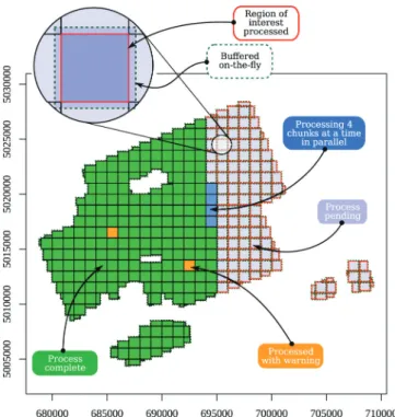
ALS data are divided into many smaller files (known as tiles) that together make a contiguous dataset covering an area of interest. The above-mentioned tools work on point-clouds loaded to memory; how-ever, real applications require upscaling of routines to facilitate pro-cessing of large datasets that do not fit into memory. A powerful engine has been developed to achieve this in lidR. Once users have designed a feature that works for a small point cloud, lidR offers the capability of applying the function over the entire coverage area using the “LAScatalog processing engine” (See section 2 and Fig. 7) that offers several features including:
•
The capability to iteratively process ‘chunks’ of any size. The chunks do not need to respect the original tiling pattern of the data acqui-sition.•
The capability to buffer each chunk on-the-fly to ensure a strict wall- to-wall output without any edge artifacts. This is particularly im-portant for terrain computations and tree segmentation, for example (Fig. 7).•
The capability to compute each chunk sequentially, or in parallel, allows lidR to take advantage of multi-core or multi-machine ar-chitectures.Fig. 5. Overview of the key components of lidR that are presented in this paper. Most functions and processing avenues within lidR are designed for user-defined
•
Automatically merging the outputs computed iteratively into a single valid object.•
Record logs and return of partial outputs in case of a crash in the user-defined routine.•
Real-time progress estimation monitoring (Fig. 7) that displays the processed, processing and pending areas.•
An error-handling manager (Fig. 7) that displays if a chunk pro-duced a warning or an error.In brief, the LAScatalog processing engine provides all the tools to apply and extend any user-defined routine to an entire acquisition, taking care of all the internal complexity of on-the-fly buffering, par-allelism, error handling, and progress estimation, etc. Users have full access to the engine with the catalog_apply() function that is also heavily used internally in almost every function. Combining the ver-satility of functions, which goes beyond the short summary provided in section 4.2, to the processing engine, a lot of processes that cannot be explored in traditional software can easily be designed by research
teams using R. A further illustration of this point can be seen in Fig. 1d where an algorithm to retrieve the position of the sensor was first de-signed and then applied to a broader area using the engine.
In summary, the versatile functions combined with the LAScatalog processing engine offer an almost unlimited number of ways in which ALS data can be processed and analysed. This adds to several other tools provided in lidR to either decimate, smooth, filter or crop point clouds, which all contribute to furthering these possibilities for the benefit of users.
4.4. Other sources of point clouds
This paper, like the overall development of lidR, focuses primarily on ALS-based methods. However, there are many other sampling sys-tems used in forestry and ecology, such as terrestrial laser scanning (TLS), digital aerial photogrammetry (DAP) or LiDAR sensors embarked on unmanned aerial vehicles (UAV), which also generate point clouds. One major issue with processing point clouds from these sources is their Fig. 6. Demonstration of the wide variety of products that can be derived using the versatile functions of the lidR package. All metrics presented here can be created
high point density, which requires a much more careful usage of memory. Considering how R is designed internally, there is very little flexibility in memory management, which makes point clouds from these alternative sources more difficult to manage. An example of the ALS-focused design of lidR is the use of an internal spatial index that is optimized for points evenly-spread on x − y axes with proportionally little variation on the z axis; this means that it will often process TLS point clouds sub-optimally. However, it does not mean that lidR
cannot be used to process other sources of point clouds. Some examples of successes in these areas include the TreeLS package (de Conto, 2019), which is designed for TLS tree segmentation and is built on top of the lidR architecture. The viewshed3d package (Lecigne, 2019; Lecigne et al., 2020) also uses lidR and TreeLS to process TLS data and address ecological questions. By paying great attention to memory usage using the tools offered by the package, we have also succeeded in integrating lidR into a DAP point cloud workflow. Fig. 8 shows the result of an individual tree detection and measurement performed in a poplar plantation. Other groups have successfully used lidR to process UAV point clouds, such as VanValkenburgh et al. (2020);Navarro et al. (2020), among others. Despite not being designed for these uses, lidR offers a versatile point cloud processing framework that enables usage beyond what it was initially designed for, either by using the existing suite of tools or by extending them.
5. Computational considerations
Expansive ALS acquisitions can result in large amounts of data that need complex processing. As a result, ALS processing software needs to be as efficient as possible when reading, writing, and processing 3D point clouds. As discussed previously, the primary goal of lidR is to create a straightforward and versatile toolbox within the R ecosystem. This choice comes at a cost of memory usage and runtime, when compared to what could be achieved with specialised software. However, a significant part of the lidR package code that drives the most demanding computations is written in C++, and is natively parallelised at the C++ level whenever possible. Memory allocations are reduced by recycling the R allocated memory whenever possible and the reliance on third-party packages is focused on efficient tools, such as the data.table package (Dowle and Srinivasan, 2019).
We have dedicated significant efforts into improving the execution time and memory usage of the lidR package. To illustrate some aspects of the package performance, we provide here some benchmarking tests that can serve, at least to some extent, as runtime comparisons with existing software. We benchmarked a selection of tools to demonstrate the computing efficiency of lidR. Tests were performed both on an Intel Core i7-5600U CPU @ 2.60 GHz with 12 GB of RAM running Fig. 7. An annotated screenshot of the live view of the lidR LAScatalog
pro-cessing engine applying a user-defined function on a 300 km2 collection of LAS
files. At the end of the process, the results are stacked to make a strict wall-to- wall output.
Fig. 8. A poplar plantation point cloud in RGB colour sampled with digital aerial photogrammetry (DAP). The red dots mark the position and height of each of the
GNU/Linux and a Xeon CPU E5-2620 v4 @ 2.10GHz with 64GB of RAM running Windows 10. The C++ code of lidR as well as other de-pendency packages were compiled with g++ with level 2 optimisation (-O2), which is the default in R packages for Microsoft Windows and most GNU/Linux distributions. We did not take advantage of the multi- core or multi-machine capabilities of the package for the results pre-sented in this paper. To ensure the reproducibility of the benchmarks, we have provided supplementary materials with an extensive set of tests that can be run on other computers to perform time comparisons. These tests include a dataset of 25 1 km2 tiles at a mean density of 3 points/m2, which was used to perform the following benchmarks and some extra multi-core parallelisation examples.
For comparisons with existing R packages, we examined how fast the lidR package performed a simple rasterisation task compared with the rasterize() function available in the raster package (Hijmans, 2019) using a set of 3 million randomly distributed points. We also compared how fast the lidR package performed a triangulation task compared to the delaunayn() function available in the geometry (Sterratt et al., 2019) package using the same set of 3 million points. Lastly, using the same data we compared how fast the lidR package performed a k-nearest neighbour (knn) search task compared with the FNN, RANN and nabor packages (Beygelzimer et al., 2019; Arya et al., 2019; Elseberg et al., 2012). The choice of these tasks comes from the fact that, (1) they correspond to recurring computational tasks that occur internally in several analyses, (2) they are computationally de-manding, and (3) they have comparable equivalents in existing R packages. Results are presented in Fig. 9 and show that lidR is 2 to 10 times faster than other tested R packages. It is the specialisation that has made lidR markedly faster than other more generic equivalent tools available in R.
However, the versatility of the package comes at a cost and a drawback is often a longer computation times and a greater memory usage. In lidR, versatile functions are offered to prototype new tools that can subsequently be implemented in pure C++, if required. For example, in the current version of the package a user can compute a simple DCM using the versatile grid_metrics() function, but lidR has a specialized grid_canopy() function that is faster by an order of magnitude (Fig. 10.a). In lidR, these ‘specialized functions’ are func-tions that could be replaced with other versatile funcfunc-tions of the package, but that were considered to be of sufficiently high interest to be specialized for much faster processing, less memory usage and, whenever possible, native parallelisation at the C++ level. Fig. 10.a shows that the specialized rasterisation tool was 50 times faster than the versatile one, yet the versatile tool remained ∼10 times faster than its equivalent from the raster package, as mentioned above.
Depending on the functions used, the reading of input files is often the primary processing time bottleneck. In comparison to the actual computation, reading LAS or LAZ files is usually slow. To demonstrate this, we measured the run times required to compute common elevation metrics in a classical ABA analysis using grid_metrics() (Fig. 10.b). This summary plot is divided to illustrate two sub-steps: (1) time spent reading the data, and (2) time spent computing metrics. The amount of runtime dedicated to reading the point cloud from files is particularly
high with LAZ files which need to be uncompressed on-the-fly. The calculations performed after the data has been loaded are compara-tively fast. It is worth recalling that lidR is able to utilise LAX files to index point clouds and dramatically speed-up on-the-fly buffering. In this example, the computation time is constant in each trial but the overall computation can be made two to four times faster if file formats are carefully chosen.
Lastly, and to provide context, we compared the processing time required to extract ground inventories, compute an average intensity image and compute and rasterise a Delaunay triangulation with FUSION and LAStools (Fig. 11) using the same test bed of 25 tiles mentioned above. This selection of comparisons was driven by the pragmatic need to ensure comparable tasks i.e. operations that are performed with the same methods and return the same outputs using all three software alternatives. In contrast to lidR, LAStools is less ver-satile but is designed to process very large amounts of data extremely efficiently (both in terms of speed and memory usage). Given the dif-ferent focus of LAStools, we expected it to perform much faster. Fig. 11 shows the results of these comparisons and it can be seen that lidR is either close to or much faster than FUSION, but always slower than LAStools; an outcome that was expected.
The goal of this set of benchmarking tests is not to identify the fastest among a set competing software tools. LAStools will always be faster than lidR by design and one may find tasks that FUSION can perform faster than lidR, and vice versa. Moreover, most tasks can simply not be compared in a direct way, such as ground segmentation or point cloud decimation, as no two software systems use the exact same methods. In addition, the tests presented here are not actually comparable. For example, we don’t know if FUSION and LAStools perform the computationally-costly tests of data integrity system-atically performed in lidR to inform users of potential errors in the data, which account for a non-negligible proportion of the computation time. Alternatively, these tests only aim to demonstrate that, despite being R-based, lidR performs comparably in many ways to existing software thanks to its C++ backend. Hence, we argue that lidR is suitable for both research purposes and operational processing of small (sub-hectare) to medium-sized (thousands of square kilometres) forest management units at least for common tasks where the methods are supported by decades of literature. However, it is important to note that
Fig. 9. Comparison of (a) Delaunay triangulation (b) k-nearest neighbour
search and (c) rasterisation with lidR and equivalent options from third party packages.
Fig. 10. Processing times for (a) rasterisation with 1 m resolution performed
with grid_canopy() (specialized) and grid_metrics() (versatile); (b) computation of common point-cloud elevation metrics using different input file formats with or without lax files to index the point cloud;
Fig. 11. Computation time of (a) 30 plots extraction from 25 files, (b) image of
the mean intensity and (c) rasterisation of a Delaunay Triangulation of the ground points.
lidR also includes some experimental tools from the literature, such as various tree or ground segmentation algorithms that are, where pos-sible, based on the original source code provided by authors, such as the CSF algorithm (see section 3.1). Consequently, in such cases, adhering strictly to the authors’ implementation means that maximum efficiency can not be guaranteed. For example, the algorithm for tree segmenta-tion developed and published by Li et al. (2012) has a quadratic com-plexity meaning that the computation time is multiplied by four when the number of points is doubled. It can therefore not really be per-formed on point clouds larger than a few hectares.
6. Downloads, current and future usage
As of August 1st 2020 the lidR package has been downloaded on average between 2500-3000 times per month. There have been eleven major updates to the package since its release in early 2017 (Fig. 12). Version 2.0.0, released in early 2019, made significant changes to the package including full integration with the R GIS ecosystem and hanced large-area processing through the LAScatalog processing en-gine. This was the starting point of a broader adoption of lidR in the academic community. The package has currently been referenced by more than 100 scientific publications mentioning the use of the lidR package for various purposes. Most reported uses relate to regular processing tasks such as DTM, CHM, ABA metrics or ground classifi-cation (e.g. Swanson and Weishampel, 2019; Almeida et al., 2019; Mohan et al., 2019; Stovall et al., 2019; Navarro et al., 2020; Cooper et al., 2020), but sometimes beyond the scope of forestry and ecology applications such as in the study of VanValkenburgh et al. (2020) where authors classified ground points in an archaeology context to capture architectural complexity of lost cities in Peru. Several reported uses also relate to gap fraction profile estimation (e.g. Senn et al., 2020). The package is otherwise regularly used for simple file processing, such as ground plot extraction (e.g. Vanbrabant et al., 2020; Mohan et al., 2019). Comparisons of algorithms from the literature included in the package are also starting to become available (Hastings et al., 2020). In addition, lidR was used as the supporting architecture for the devel-opment of new packages such as TreeLS (de Conto, 2019; de Conto et al., 2017) and viewshed3d (Lecigne, 2019; Lecigne et al., 2020), two packages dedicated to TLS processing. Overall, reported uses show
that the package has been used in a large range of ecological contexts, such as tropical rain forest (Almeida et al., 2019), subtropical forest (Sothe et al., 2019), boreal forest (Tompalski et al., 2019a), savanna (Zimbres et al., 2020) and many others.
The latest stable release of lidR can be downloaded from CRAN and is shipped with a 150-page comprehensive user-manual that con-tains hundreds of reproducible examples simply by copy-pasting a few lines of code and can be installed with the command in-stall.packages("lidR"). The user can reproduce most of the ex-amples shown in this paper using only this user-manual. In addition to the user-manual (which is the only official source of comprehensive and consistent documentation), some extra and often more user-friendly sources of information, usually in the form of tutorials can be found on Internet. The lidR book, which can be found at https://jean- romain.github.io/lidRbook/ is a guide that contains tutorials for both new and advanced users. Users can also find help from the com-munity at https://gis.stackexchange.com/ using the lidr tag that currently hosts more than 100 questions.
The package being in constant evolution, new features are already in development, such as support for full waveform data, processing speed improvements, additional methods from the peer-reviewed lit-erature, new methods for mapping water bodies, forest roads segmen-tation, power line and transmission tower segmensegmen-tation, and versatile tools for mesh processing. We also aim to provide better support for processing TLS data by implementing a 3D spatial index that is suitable for this type of point cloud.
7. Conclusion
The use of ALS data for forestry and ecological applications, in-cluding the derivation of highly detailed and accurate terrain models, canopy height model development, and forest inventory estimation at both the plot- and individual tree-scale, is well established, with many researchers and managers regarding ALS as a mature and im-plementable technology that can be applied in an operational context. Considering the rapid integration of the technology globally, ALS pro-vides a key success story of the evolution of a new technology from research and development to production.
A simple scan of the available software platforms to process ALS data, however, demonstrates that while the technology is mature, the use of validated, repeatable, transparent and readily available tools is not.
In this context, the lidR package provides a significant set of al-gorithms implemented from the peer-reviewed research literature. We showed that lidR always provides at least two options for any given task to enable users to rely on potential alternatives when one method does not suit a given scenario. Also, lidR aims to provide a space where new algorithms can be tested. By making the methods from the literature available within the package, we intend to enable the com-munity to figure out their strengths and weaknesses across various contexts, which may (or not) eventually lead to wider adoption. In other words, lidR is designed as a laboratory software.
This design choice makes lidR different to other existing software but its open-source and cross-platform nature, its ease of use and its versatility already make it broadly accepted by the research commu-nity, as evidenced by the numerous citations of the package in the peer- reviewed literature, as well as some newly developed tools based on the lidR architecture not only focused on ALS point clouds but also TLS, UAV and DAP point clouds.
Declaration of Competing Interest
None. Fig. 12. Monthly and total downloads of the lidR package since its release.
Data obtained from the cranlogs package (Csárdi, 2019) in R. The red line indicates monthly downloads, while the blue dashed indicates cumulative total downloads.