Ada : context-sensitive context-sensing on mobile devices

(1)

Ada: Context-Sensitive Context-Sensing

on Mobile Devices

by

Yu-Han Chen

MASSACHUSETTS INSE OF TECHNOLOGY

JUL

0 8 2013

LIBRARIES

B.S., Computer Science and Information Engineering (2010) National Taiwan University

Submitted to the Department of Electrical Engineering and Computer Science in partial fulfillment of the requirements for the degree of

Master of Science in Electrical Engineering and Computer Science at the

MASSACHUSETTS INSTITUTE OF TECHNOLOGY

June 2013

@

A u th or ... ...

Department of Electrical Engine ing and Computer Science

May 10, 2013

/A

Certified by ...

Hari Balakrishnan Professor of Electrical Engineering and Computer Science Thesis Supervisor

Accepted by ... . . ..

Leslie A. Kolodziejski Chair of the Committee on Graduate Students

(2)

(3)

Ada: Context-Sensitive Context-Sensing on Mobile Devices

by Yu-Han Chen

Submitted to the Department of Electrical Engineering and Computer Science on May 10, 2013,

in partial fulfillment of the requirements for the degree of Master of Science in Electrical Engineering and Computer Science

Abstract

This thesis describes the design, implementation, and evaluation of Ada, a context-sensing service for mobile devices. Ada explores new points in the accuracy-energy-responsiveness design space for mobile context sensing. The service exports an API that allows a client to express interest in one or more context types (mode-of-movement, indoor/outdoor, and entry/exit to/from named regions), and subscribe to specific modes within each context (e.g., "walking" or "running", but not any other movement mode). Each context type in Ada can be in one of a set of mutually exclusive states. Each context has a detector that returns its estimate of the mode. To achieve high accuracy and low energy consumption, the detectors take both the existing context and the desired subscriptions into account, adjusting both the types of sensors and the sampling rates. To accurately determine the movement mode, Ada uses a new peak frequency feature from acceleration magnitudes, combining it with two other features. We present results from trace-driven experiments over carefully labeled data from real users, finding that our mode-of-movement detector achieves an accuracy of

93%, out-performing previous proposals like UCLA (55%), EEMSS (83%) and SociableSense (72%), while consuming between 2 and 3x less energy.

Thesis Supervisor: Hari Balakrishnan

(4)

(5)

Acknowledgments

First of all, I would like to express my deepest gratitude to my advisor, Hari Balakrish-nan, who has provided me with immeasurable opportunities and constant support. I have been greatly inspired by his wisdom, creativity, and vision. Doing research is challenging,

but his guidance always prevents me from heading into possible catastrophes, his optimism encourages me to conquer all the difficulties ahead, and his recognition makes every effort worthwhile. Outside of research, he is so down to earth and humorous that you might

some-times forget he is one of the leading computer scientists in the world.

My thanks go to my academic advisor, Daniela Rus; her advice has been a great help

in both academic studies and life. I still remember when she shouted "tough girl" at me as

I decided to take two TQE classes in my first semester; believe it or not, those two words

tremendously boosted my confidence, and helped me get through my hardest times at MIT. Also, I would like to offer my special thanks to Li-Shiuan Peh and Sam Madden, for their warm support, and encouragement in many unexpected ways.

To my undergraduate advisors, Hao-Hua Chu and Polly Huang, they are the reasons that brought me here to MIT. They boldly offered me the opportunity to take part in the PipeProbe project as an undergraduate student, despite the fact that I knew nothing about research. They guided me through each step in completing a paper, and put all of their trust in me to excel. I will always be thankful for their support and recognition.

My thesis work would have never been possible without the help from my amazing

col-laborators. I am particularly grateful for the assistance given by Anirudh Sivaraman. He contributed generously to this project, helped me design and implement the system, corrected my writing, and taught me all the skills required to be a better coder. Most importantly, he is always willing to spend time chatting with me, sharing his life experiences, and providing advice on how to get the most out of the PhD experience and maintaining a healthy and happy life at the same time. I thank Lenin Ravindranath - for being a key person on this project. His knowledge and inspiration in this field are simply invincible. Without his advice and persistence, this work would not have been so successful. To Somak Das, for assisting me in completing all of the experiments. Working with him has been a lot of fun, and I

(6)

will never forget the afternoon we spent together in zero-degree weather attempting to get a GPS fix. To Alvin Cheung - the king of free food - thanks for being the best mentor, guiding me through disappointments, pointing out flaws in my ideas or algorithms, providing me numerous survival tips, and letting me believe everything is possible.

My special thanks are extended to my labmates in the NMS group. Shuo Deng has greatly

helped me adapt to the research environment at MIT. She patiently taught me how to use the power monitor (more than two times), graciously listened to my grumbles, and shared many secret discounted deals with me. Katrina LaCurts is the person who brings fun into the lab. Without her, the plants in our office would never have gotten their names, the NMS group would never have had a group outing, and the whiteboard eraser would never have found its wonderful home. She is the one who turns the intense atmosphere at MIT into something a lot more playful and loving. Keith Winstein, one of the brightest men I have ever met in my life, is very selfless. He is always ready to share his wisdom and experiences with others, and he tries hard to help everyone find ways to enjoy their PhD life like he does. I especially thank him for the feedback on my paper drafts, all his comments hit the nail on the head and made me clearly understand what I should do to improve it. I would also like to thank Raluca Ada Popa for giving me the shirt with her superpower, Victor Costan for teaching me how to give an impressive short talk, Jonathan Perry for many fruitful research discussions, and Ravi Netravali for all the fun NBA chats.

I would also like to thank many of my friends who fill my MIT experience with happiness.

Their company is a constant reminder that there is much more to life than research. To Ann Lee, for being as such a wonderful friend, putting up with all my bad jokes, and buying me food when I am suffering with a deadline. I enjoy the time we spend together trying to prove a language is NP-complete, attending the most relaxing PE class, exploring new restaurants, and supporting each other through ups and downs. To my roommate, ShinYoung Kang, who has been the greatest victim of this work. Thanks for never being exasperated with my late hours and dirty dishes. And thanks for being like a mom, reminding me to maintain a better work-life balance, educating me about the common sense in everyday life, and listening to my frustration with care and understanding. To Kai-Chien Yang, for the friendship in the past twelve years. She creates a home away from home for me and is always there for a

(7)

chit-chat, gossip, and many laughs. Furthermore, I thank Chia-Hsin and Yu-Hsin for helping me pass my TQE, Shu-Heng for organizing all the wonderful gatherings, Yehes and Chern for collecting a huge amount of biking and running data for this project, and Hsin-Jung, Pan, Kevin, Marcus, and Tony for filling my life with many smiles.

Last and most importantly, my deepest thanks to Dad, Mom, Kimberly, and my family,

I owe you everything for making me the person I am today. It is your encouragement that

motivates me to keep marching ahead and it is your endless support that makes all this possible. I also thank little Senya and Vasya, for bringing tremendous joy into my life. Finally, I would like to thank Erh-Kang Tsao, for always believing in me, giving me all you have, and loving me as the way I am. It is just a miracle to have you in my life.

(8)

(9)

List of Figures

3-1 Ada's architecture . . . . 27

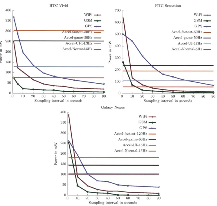
3-2 Power consumption of different sensors on three phone models (HTC Vivid, HTC Sensation, and Samsung Galaxy Nexus) . . . . 29

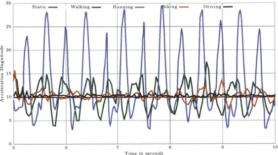
4-1 Time series of acceleration magnitude . . . . 34

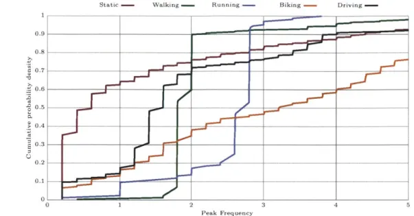
4-2 CDF of peakf frequency . . . . 35

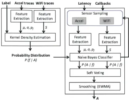
4-3 Mode-of-movement detector processing algorithm . . . . 36

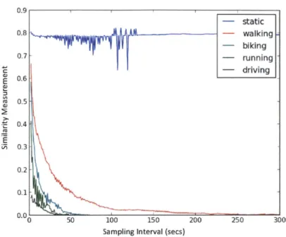
4-4 Estimating user's speed of movement using the similarity between two WiFi fingerprints under different sampling intervals. When the user is static (driv-ing), the similarity between two consecutive WiFi fingerprints are high (low) across all sampling intervals . . . . 37

6-1 Accuracy as a function of subscription. Ada achieves higher accuracy than other schem es always . . . . 53

6-2 Energy consumption as a function of subscription. Ada consumes lower energy than other schemes always . . . . 54

6-3 Energy and accuracy versus latency. Ada's mode-of-movement detector trades off latency of detection for decreased energy consumption while maintaing the sam e accuracy . . . . 56

6-4 The effect of combining accelerometer with WiFi/GPS and smoothing . . . . 58

6-5 Geofence power percentiles. Ada's geofence detector consumes low energy and its energy consumption increases as the number of geofences increases . . . . 60

(12)

(13)

List of Tables

1.1 Accuracy and energy consumption of different mode-of-movement schemes. Ada's mode-of-movement detector outperforms previous proposals like UCLA* [48],

EEMSS* [57], and SociableSense* [42], while consuming between 2 and 3x less

energy ... ... 17

2.1 Features of related systems in activity detection using mobile devices . . . . 21

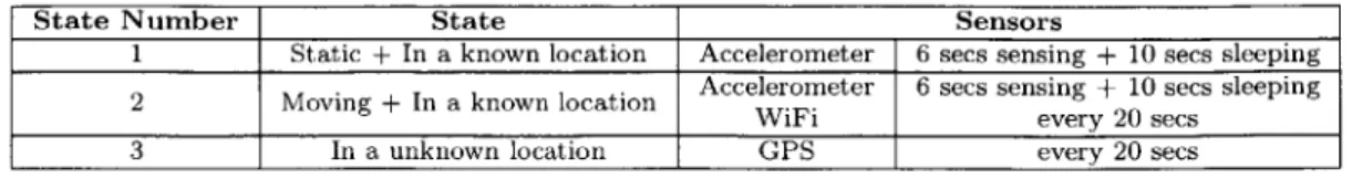
3.1 Ada's context detectors and the sensors used in each of the detector . . . . . 28

5.1 The state machine of EEMSS . . . . 49

6.1 The features and their corresponding KDE variances (h2_{) used in Ada's} mode-of-movement detector. We use cross-validation on the training set to obtain the best set of parameters, and freeze them before we see the testing data . . 52

6.2 % accuracy with feature subsets, static callback . . . . 57

6.3 % accuracy with feature subsets, all 5 callbacks . . . . 57

6.4 % accuracy while adding other features . . . . 59

(14)

(15)

Chapter 1 Introduction

For about two decades, the mobile computing community has recognized that the ability to infer a mobile user's context (i.e., properties of the user's activity and location) is useful in a wide range of mobile applications. Some examples include situated messaging [44], location-aware advertising [6, 19], and lifelogging [21, 27, 10]. Several papers have been published on detecting user activity and location-based attributes (see Chapter 2). Despite this significant work, however, there is no easily usable context-sensing service available on standard smartphone platforms. There are a few reasons for this. First, current context recognition systems are not accurate enough to provide a general context-sensing service; second, most systems are not energy-efficient in how they use the mobile device's sensors and process sensor data; third, none of the prior work exposes context detection as a programming abstraction. This work describes the design, implementation, and experimental evaluation of Ada, a system that provides an accurate and battery-efficient context-sensing service with a simple API for Android and Windows Phone devices.

Ada provides three context detectors: (1) mode-of-movement, which determines if the user is static, walking, running, biking, or driving; (2) indoor/outdoor, which determines whether the user is inside or outside a building; and (3) geofences, which determines if the user has entered or exited one of a set of named location-based regions. Ada is extensible to allow other detectors, which could reuse the implemented sensor processing and fusion methods.

(16)

states), but the user can be in only one mode at any time. This restriction simplifies the API, and provides opportunities to reduce energy. A client subscribes to one or more contexts and to one or more modes within each context. For example, a background tasking application could subscribe to "walking" or "running" in the movement context, and to "outdoor" in the indoor/outdoor context; the results may be used to log the total time or distance covered by the user in walking or running outdoors.

Ada incorporates the concept of context-sensitive context sensing in depth and applies two themes in its design and implementation:

1. Its detectors determine the sensors to use and the sensor sampling rates taking client

subscriptions into account. If the client is interested in walking or running, the sensor sampling rates are different from if the client is interested in biking or driving, for example.

2. Its detectors determine the sensors and sampling rates taking the current mode into account. For example, the geofence detector uses its distance from the nearest geofence in deciding which sensors to sample.

A mobile context-sensing service generally has to navigate a design space that has different

trade-offs between detection accuracy, energy consumption, and responsiveness. We define the accuracy of a context detector as the fraction of time when it returns the desired mode correctly. The energy consumed is obtained by measuring the power consumption of different sensors at various sensing rates across different phones, and keeping track of the amount of time spent at each sensing rate, and on a variety of smartphones. The responsiveness is a requirement from the client, which tells Ada how often it wants to be notified.

It is difficult to evaluate context-sensing systems in practice. We develop a rigorous and reproducible experimental method, which does not depend on the specific algorithms used in the context detectors. We gather several carefully labeled traces from real users in different contexts, and stitch them together in our evaluation; the method is in contrast to previous work that shows a specific window of data from one context mode or activity and evaluates the fraction of time the detector gets it correct. By contrast, our method provides a stream of sensor readings across different modes or activities evaluates the detector on how often, within a specified response rate, it gets the answer correct. Our evaluation spans over 50

(17)

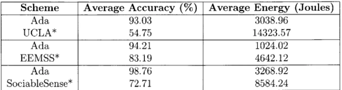
Scheme Average Accuracy

(%)

Average Energy (Joules) Ada 93.03 3038.96 UCLA* 54.75 14323.57 Ada 94.21 1024.02 EEMSS* 83.19 4642.12 Ada 98.76 3268.92 SociableSense* 72.71 8584.24

Table 1.1: Accuracy and energy consumption of different mode-of-movement schemes. Ada's mode-of-movement detector outperforms previous proposals like UCLA* [48], EEMSS* [57], and SociableSense*

[42],

while consuming between 2 and 3x less energy

hours of trace data drawn from ten users. Table 1.1 summarizes our main results for our mode-of-movement detector.

In addition to the idea of context-sensitive sensing, a simple API with mutually-exclusive subscription modes, and a novel experimental evaluation method, this thesis explains why certain features drawn from the sensed data perform better than others. The mode-of-movement detector is of significant interest both because of its many uses and because of much prior work on the problem. We find that three features, which all work over the time-windowed magnitude of the three-axis acceleration sensor data: the mean, standard deviation, and peak frequency (a feature that we propose here), work better than numerous other previously proposed features.

(18)

(19)

Chapter 2 Related Work

There has been a variety of related work in the area of context-sensing. To illustrate clearly the contribution of Ada and each of Ada's detector, we divide related work into three main areas: activity detection, energy-efficient activity abstractions, and location-based context detection.

2.1 Activity Detection

Many systems exist to infer human motion activities, movement modes, or postures. Related work in this domain can be grouped based on the types of devices used to implement the system: custom wearable sensors and mobile devices. In this section, we discuss each category in detail with information on how Ada's mode-of-movement detector builds on or differs from the ones described.

2.1.1 Custom Wearable Sensors

A majority of research has investigated various methods to determine user's activity using

customized wearable sensors. Farringdon et al. [15] builds a wearable sensor badge with two two-axis accelerometers to determine whether a person is sitting, standing, lying, walking, or running. To differentiate between sitting, standing, and lying, they examine the raw accelerometer reading of each direction and determine the orientation of the accelerometer. To further distinguish between running and walking, they use the difference between the

(20)

maximum and minimum reading of each direction and count the number of times it crosses the average value. However, no experimental results are presented in the paper.

Randell and Muller [43] use a two-axis accelerometer to determine if the user is walking, running, sitting, walking upstairs, downstairs, or standing. The sensor is worn in the trouser pocket with a fixed orientation and sampled at a low frequency (5 Hz) to save energy. From the samples they extract four features including the root mean square and the integration of both axes over the last 2 seconds. They then use a clustering algorithm to infer the user's activity. With data collected from 10 users, their results shown that they can infer the user's activity with 85-90% accuracy.

Kern et al. [23], unlike the two previous systems that try to find recurring patterns in the data, this work models the activity explicitly. They mount twelve three-axis accelerometers to all major joints on the human body to capture user's postures and activities (sitting, standing, walking, upstairs, downstairs, shake hands, write on board, and keyboard typing). Data is sampled at a rate of 92 Hz, and the mean and variance are computed over a window of 50 samples. The paper also investigates the number and placement of sensors and finds out that for "leg-only" activities, such as walking or stairs, sensors on the legs, e.g. hip, are sufficient.

Bao and Intille [8] develop an activity recognition system to identify twenty activities using two-axis accelerometers placed in five locations on the user's body. This work shows that placing an accelerometer at only two locations (either the hip and wrist or thigh and wrist) did not affect activity recognition accuracy significantly compared to a system with five sensors. Ganti et al. [16], and Gyorbiro et al. [17] also mount multiple accelerometers on different positions on the body to infer a range of activities. Work by [16] further investigates the amount of storage needed without loss of the precision of data collected. They observe that when the user is walking, the number of footsteps taken were between three and six every second. Hence, based on Nyquist's sampling theorem, they propose that the minimum

sampling rate should be at least 25 Hz.

Most work in this domain shares the same goal with Ada - providing better services or applications by being cognizant of user's movement activities or modes. Unfortunately, wearable devices with a fixed placement are too obtrusive and are inconvenient. Even though

(21)

System Movement Modes Sensors Kwapisz et al. [26] Walking, Running, Ascending stairs, Descending stairs, Sitting, Standing Accelerometer 20 Hz

Miluzzo et al. [34] Sitting, Standing, Walking, Running Accelerometer 32 Hz

Sohn et al. [50] Static, Walking, Driving GSM 1 Hz

Anderson et al. [7] Static, Walking, Driving GSM

-LOCADIO [25] Static, Moving WiFi 3.2 Hz

Zheng et al. [58, 59] Walking, Driving, Taking a bus, Biking GPS 0.5 Hz Stenneth et al. [51] Static, Walking, Biking, Driving, Taking a train GPS Every 15 secs

Mun et al. [36] Static, Walking, Running, Driving WSM 0.5 Hz

Reddy et al. [48] Static, Walking, Running, Biking, Driving Accelerometer 32 Hz

GPS 1 Hz

Accelerometer

TransitGenie [53] Static, Walking, Driving WiFi Adaptive

GPS

SociableSense [42] Static, Moving Accelerometer Adaptive

Accelerometer

EEMSS [57] Static, Walking, Driving WiFi Adaptive

GPS

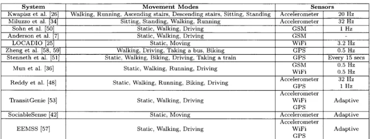
Table 2.1: Features of related systems in activity detection using mobile devices

installing multiple sensors on the human body provides more detailed information, it is only practical for specialized applications and services. Ada differs from most prior work in that we use sensors available on a commodity smart phone along with relaxed requirements on how the device should be worn in addition to being orientation, position, and user agnostic.

2.1.2 Mobile Devices

Mobile devices are increasingly capable of rich multimodal sensing. Today, a wealth of sensors including camera, microphone, GPS, accelerometers, proximity sensors, pressure sensors, and light sensors are already standard. on mobile devices. As a result, researchers are looking to use mobile device as a platform for activity detection. Table 2.1 summarizes the features of related systems in activity recognition using mobile phones.

Many research projects have focused on using the three-axis accelerometer on mobile devices to infer user's activity. Kwapisz et al. [26] aims to infer six activities with forty-three features. This work compares the performance of different classification algorithms and discovers that the multi-layer perceptron performs better than the decision tree and the logistic regression. CenceMe

[34]

infers user's current activity with fewer features. It finds that the mean, standard deviation, and the number of peaks per unit time are enough to tell between static, walking, and running. Using the decision tree as the classifier, CenceMe achieves 70-80% accuracy. However, both systems assume the phone is in user's pocket. They

(22)

also do not attempt to detect biking or driving.

Some approaches to detecting human movement modes have used radio signals from GSM or WiFi. Sohn et al. [50] uses the rate of change in GSM cell tower observations to infer whether a user is stationary, walking, or driving. The inference is then used to approximate the user's daily step count. In [7], similar experiments are carried out by further exploiting the knowledge of human normal behavior with a Hidden Markov Model (HMM). It also investigates the impact of environment (metro versus suburban) on the detection performance and discovers that the system achieves better performance in a suburban environment because people tend to drive at a faster speed than in the metro environment. Even though scanning

GSM fingerprints is energy-efficient, GSM fingerprints aren't universally available across all

phones. Some phone models limit the cell information to only the connected tower or do not make it available at all. Moreover, GSM based activity detection systems are unlikely to be able to properly distinguish between activities with similar speed. WiFi based systems, like

LOCADIO [25], measure the variation of the signal strength of access points to determine

whether or not the user is in motion.

Several systems rely on GPS for sensing movement modes. For instance, Zheng et al. [58,

59] combine GPS with a post-processing step that uses likely transportation modes from a

corpus of contributed data for classification. Alternatively, Stenneth et al. [51] combines GPS with GIS information, such as the real-time bus locations, spatial rail and spatial bus stop information. They find that speed is the most effective feature from GPS to infer movement modes. Liao et al. [28] builds personalized models based on learning destinations and routes from historical data to build transportation mode classifiers. Unfortunately, GPS based systems consume significant amount of energy and do not work when the device is indoors. Also, GPS-only solutions perform poorly when classifying of movement modes with similar speed, such as running, biking, and slow driving.

Other work integrates multiple sensors on the mobile device to determine a user's activity. Mun et al. [36] uses the connected GSM cell tower information with the additional of fea-tures derived from WiFi observations for classification. TransitGenie [53] uses data from the accelerometer, WiFi, and GPS to distinguish walking from driving, and uses the prediction to estimate the arrival time of buses. To determine which sensors to use and their sampling

(23)

rates, it maintains a finite state machine and only turns on power-hungry sensors only if it is needed. Ada also adopts this notion, but is able to detect more mobility modes.

Closest to our work is Reddy et al.'s work from UCLA [48] (which we will refer to as

UCLA* in this thesis), which uses GPS and accelerometer readings for transportation mode

inference. This work includes a comprehensive evaluation of the energy and accuracy of the system under various scenarios. We find that Ada outperforms UCLA* in our evaluation on both accuracy and energy. Ada also combines the information from multiple sensors. How-ever, unlike previous work, it adapts the choice of sensors and their sampling rates based on feedback from the detector. We observe that acceleration data, by itself, is good to capture movements, but distinguishing biking from walking and driving is a vexing problem. Aug-menting the acceleration-derived features with approximate speed estimates could help this distinction. Therefore, Ada relies primarily on acceleration data, uses WiFi to approximate speed, monitors the density of WiFi APs, and only turns on GPS when WiFi APs are not visible.

2.2 Energy-Efficient Activity Abstractions

Several research projects aim to build an energy-efficient activity recognition system through intrusive instrumentation of the user or a user's surroundings using sensor boards [56, 52,

31, 22], on-body accelerometers [9, 33, 45], or RFIDs [41]. Instead, our system focuses on

activity recognition using commodity smart phones. Systems such as SociableSense [42], Kobe [11], and EEMSS [57] explore energy-accuracy-latency tradeoffs in sensing applications running on smart phones. SociableSense provides an adaptive sampling mechanism using a learning technique based on the theory of learning automata to control the sampling rate of the accelerometer. It maintains a probability of sensing to determine the sampling duty cycle of the accelerometer. The sensing probability is then updated based on the result of sensing action. EEMSS adopts the strategy of hierarchical sensor management to recognize user states as well as to detect state transitions. Its goal is to power only a minimum set of sensors and use appropriate sensor duty cycles to improve device battery life. Ada is motivated by the same end goal of energy-efficiency, but, our approach is different. We

(24)

compare Ada to both SociableSense and EEMSS (which we will refer to as SociableSense* and EEMSS* in this thesis) and find that we outperform both systems on both energy and accuracy.

Google [1] recently launched an activity detector API for Android. Its emergence reveals the desperate need for exposing context detection as a programming abstraction. The service detects if the user is currently on foot, in a car, on a bicycle, or static. The service allows applications to request periodic activity recognition updates. For each update interval, the service sends a list of possible activities and the probability of each one to the application. The activities are detected by periodically waking up the device and reading short bursts of low power sensor data to save energy. We are planning to compare this system with Ada's mode-of-movement detector.

SeeMon [22] achieves energy-efficiency in the context of multiple external sensors attached to a computation device; they do not evaluate their system on mobile phones. ACE [37] uses a different approach, by detecting low energy proxy activities that correlate with the activity that needs to be detected. Ada's approach is complementary and can be applied to the proxy detectors in ACE. Our approach of context-sensitive sensing may be viewed as a significant generalization of triggered sensing

[35).

2.3 Location-Based Context Detection

Several systems reduce the energy cost of localization using a variety of techniques. Some systems [60, 32] adapt their sampling rate to reduce energy cost. A-Loc [29] uses the obser-vation that the required location accuracy varies with location. Where possible, RAPS [38] uses historical data along with the accelerometer in lieu of GPS. CAPS [39] and CTrack [55] sequence cellular base stations to retrieve approximate position. Cleo [30] offloads all GPS signal processing to the Cloud to reduce energy consumption, but requires a modified GPS board to support offloading, increases wireless energy consumption a little (and adds latency). EnLoc [12] allows the client to pick an energy budget which it then uses to achieve the best accuracy subject to the energy budget constraint. Ada's geofence detector can use these schemes as a blackbox, by deciding when to query them for location, without worrying about

(25)

how they work internally. SensLoc

[24]

shares Ada's goal of detecting named locations, but works best only when the user visits the same location repeatedly.

(26)

(27)

Chapter 3 Design Overview

In this chapter, we describe the architecture of Ada, the services it provides, and the energy profile of various sensors that guides the design of the system.

3.1 Ada's Architecture

Latency Subscribe Calbacks

11l

1' I

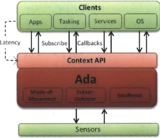
Figure 3-1: Ada's architecture

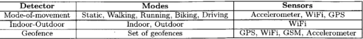
Figure 3-1 shows the design of Ada and Table 3.1 tectors. A client subscribes to one of several available detectors. For instance, a client using movement hints (e.g. [46]) might only be interested in monitoring if the

shows the sensors used in Ada's de-callbacks from any of Ada's context to enhance the performance of WiFi user is static or not. Alternatively, a

(28)

Detector Modes Sensors

Mode-of-movement Static, Walking, Running, Biking, Driving Accelerometer, WiFi, GPS

Indoor-Outdoor Indoor, Outdoor WiFi

Geofence Set of geofences GPS, WiFi, GSM, Accelerometer

Table 3.1: Ada's context detectors and the sensors used in each of the detector

fitness application calculating a user's daily calorie expenditure might be interested in all five callbacks from the mode-of-movement detector. Clients also specify the latency of detection, which specifies how often Ada returns a callback to the client. For example, a reminder application might need to notify the user within a few seconds while a trajectory logging application can tolerate a longer detection latency before it starts logging samples.

We intentionally use the term "client" rather than "application" or "process" because Ada's APIs support several different use cases. For example:

1. The client could be tasking applications or services [47] that run in the background.

These applications run continuously in the background, triggering actions based on the activities. For instance, the tasking application might want to log certain sensory data whenever the user starts running.

2. The client could be a foreground applications such as a web browser or chat plugin. In such cases, the foreground application could adapt its user interface to the activity of the user.

3. The client could be the operating system itself. This scenario is useful when we want

to change system behavior (like turning off the screen or setting "airplane" mode) automatically. Ada can also help wireless protocols by providing contextual hints [46]. Ada maintains a list of clients that have subscribed to each of the modes that Ada's detectors provide. It runs only one instance of a specific detector for each phone and conveys callbacks from the context detector to their respective clients.

3.2 Power Consumption in Context Sensing

To understand the power consumption of sensors on a phone, we performed experiments to quantify the power consumption of GPS, WiFi, GSM, and the accelerometer on three phone models (Samsung Galaxy Nexus, HTC Vivid, and HTC Sensation). We wrote an

(29)

400 700

-WiFi WiFi

350 GSM 600 GSM

GPS - GPS

-300 Acce1-Tastest- Muz -500 Accel-fastest-50Hz

-Accel-game-5OHz - Accel-game-50Hz -250 Accel-UI-14.3Hz -Accel-U-17Hz S 5 ~~~400 Acl1IlH 200 Accel-Normal-5Hz - Accel-Normal-5Hz -300 00 A 150 100 200 -50 100 -0 01 0 10 20 30 40 50 60 70 80 90 0 10 20 30 40 50 60 70 80 90 Sampling interval in seconds Sampling interval in seconds

Galaxy Nexus 400 WiFi -350 GSM -GPS 300 Accel-fastest-120Hz -Accel-game-60Hz -250 _{Accel-UI-15Hz} 200 Accel-Normal-15Hz-0 c 150 100 50 0 0 10 20 30 40 50 60 70 80 90 Sampling interval in seconds

Figure 3-2: Power consumption of different sensors on three phone models (HTC Vivid, HTC Sensation, and Samsung Galaxy Nexus)

(30)

Android application to continuously sample the sensor at a given sampling interval. For the accelerometer, we set the mode to each of FASTEST, GAME, UI, or NORMAL. For WiFi and GSM, we used Android's AlarmManager to schedule a periodic WiFi scan at the specified sampling interval. When the alarm fires, the Android application asks for the names and RSSIs of neighboring WiFi APs (access points) or cell towers. For GPS, we used the Android LocationManager API to specify a sampling interval. We conducted GPS measurements in an open space with good GPS reception to ensure the GPS would acquire a lock.

To accurately measure power consumption of the sensors alone, we halted all running applications, turned off the screen, used the Monsoon Power Monitor to deliver a constant voltage of 3.7V, and measured the long-term average power consumption. The power profiles for three phone models are shown in Figure 3-2.

We make three observations. First, there is a clear difference in the power consumption of different sensors. For instance, on the HTC Vivid, at a sampling interval of 5 seconds,

GSM is more than 6x as energy-efficient as GPS.

Second, depending on the sampling interval, WiFi scans on the Sensation, for instance, can consume anywhere between 16 mW and 640 mW.

Third, the accelerometer power consumption increases with sampling rate despite the fact that the accelerometer is itself a low-power sensor. The reason is that Android currently re-trieves accelerometer samples by polling the accelerometer at the specified sampling rate. So, the power consumption measured reflects the power consumption of a CPU polling a periph-eral for I/O at the specified sampling rate. This could be easily fixed if the accelerometer's samples were batched and transferred to main memory every second using Direct Memory Access (DMA).

These observations guide our context-sensing methods. The first observation shows that picking sensors based on the specific subscriptions will save energy. The second observation shows that being selective about the sampling interval for a particular sensor is useful. Finally, because the power consumption of the accelerometer goes up with the sampling rate, we do not use a sampling rate higher than 40 Hz.

The measurements above ignore the cost of computation. Any context-sensing algorithm will involve some computation in addition to the sensing itself. For instance, it is common

(31)

to window the data to compute specific statistics (such as mean, and variance). Normally, the windowing interval is on the order of a few seconds. The interval between successive predictions from a context sensing schemes is on the order of tens of seconds. At these time scales, computation energy is insignificant compared to sensing energy.

(32)

(33)

Chapter 4 Context Detectors

In this chapter, we describe the algorithm of the mode-of-movement detector, the indoor-outdoor detector, and the geofence detector. We also illustrate the observations that guide the design of the techniques presented in this chapter.

4.1 Mode-of-Movement Detector

This detector determines which one of five movement modes-static (S), walking (W), run-ning (R), biking (B), or driving (D)-a mobile device (user) is in. A client runrun-ning on the mobile device may subscribe to any subset of these modes, specifying a response interval, L; in return, the detector returns its best estimate of the movement mode every L seconds. The movement-mode detector uses data from the three-axis accelerometer, and if available, augmented with data from WiFi position sensors or from GPS. All these sensors are sampled with energy-efficiency in mind, so the amount of data from GPS will be small or non-existent in many cases.

One prior approach to detecting the movement mode (also called "activity" in some earlier work) is to use GPS velocity [48, 57]. Unfortunately, this approach is problematic even when battery life is not a concern because GPS is unavailable indoors, and because vehicles may move at biking or even slower speeds in heavy traffic. Ada supports both indoor and outdoor uses, relying primarily on acceleration data. It uses WiFi to approximate "speed" and GPS when WiFi APs are not visible.

(34)

30 25 20 so 15 0 5 0

Static - Walking - Run ing - ik ing - Driving .

5 6 7 8 9 10

Time in seconds

Figure 4-1: Time series of acceleration magnitude

The main contributions of our movement detector over prior schemes are: (1) the use of a new peak frequency feature from the acceleration data, used in conjunction with two other known features, (2) a processing algorithm (summarized in Figure 4-3) that combines the different features of a feature vector from one sensor using the Naive Bayes classifier, and fuses the outputs of different sensors using soft voting, and (3) an adaptive sensor sampling method that takes both the subscribed callbacks and current mode into consideration to reduce energy consumption. The rest of this section describes these ideas.

4.1.1 Features

The detection problem is a multi-label classification with the labels being S, W, R, B, and D, the five modes mentioned above. For data collected from each sensor, the detector computes feature vectors over which the training phase and online learning method can work.

Accelerometer. As in prior work, we compute the magnitude, Va

+

a7.

+

a z, of each

three-axis accelerometer reading. The intuition for this calculation is shown in Figure 4-1, which shows the time series of the magnitude for different movement modes. One can see that many of the modes of interest "look different" on this chart. For example, running has the highest standard deviation when computed over a time window of a few seconds, so

(35)

Static - Walking - Running . 0.69 0.1 ---- --- -0 04._________ _ 03 0 1 2 3 4 5 Peak Frequency

Figure 4-2: CDF of peakf frequency

it might be possible to use the windowed standard deviation as a useful feature. So does walking, but people generally walk slower than they run, so one might be able to distinguish between those two modes by looking at the frequency-domain version of the same data and seeing if they peak at different frequencies. Plotting the frequency spectrum does show a spike around 1 Hz to 2 Hz, whereas biking and driving are more evenly spread over a wider frequency range.

This intuition suggests that we want a feature to capture the periodic behavior, another to capture the overall strength of the acceleration (while static, gravity is the only force acting, while other modes will have differing magnitudes), and another to capture the variation of these magnitudes. There are numerous possible features one could construct and try out. We experimented with many possibilities, inspired by previous work on activity detection as well as signal processing methods used in medicine. These features include:

1. Mean acceleration magnitude, ji, calculated over non-overlapping windows of T = 5 seconds, previously investigated by [32].

2. Standard deviation, o, of accelerometer magnitudes calculated over the same win-dows [53, 48, 42, 57].

3. The peak non-zero (non-DC) frequency, pf, of the acceleration magnitudes computed

over the same time window using the FFT.

(36)

Driving-Probability Distribution P (f /A) Latency Callbacks Sensor Sampling Feature Feature Extraction Extraction M, a, Pf S

Naive Bayes Classifier P (A / fl P (A / f)

Soft Voting

Smoothing (EWMA)

A

Figure 4-3: Mode-of-movement detector processing algorithm

4. The spectral coefficient of the magnitude of the three-axis acceleration data samples at

1 Hz, 2 Hz, and 3 Hz [48].

5. The spectral entropy of the DFT of accelerometer magnitudes over a time window of

T = 5 seconds [32].

6. The peak power ratio of the DFT of the accelerometer magnitudes computed over a

window of T = 5 seconds [53].

7. The line length (or curve length), defined as the sum of the absolute value of the differ-ence between two successive acceleration magnitudes, computed over non-overlapping windows of T = 5 seconds. This feature has been used successfully in seizure

detec-tion [14].

8. The average nonlinear energy, defined as the average value of xo - x_-xi1 1, computed

over non-overlapping windows of T = 5 seconds [20].

We conducted controlled experiments with various combinations of the above features, and empirically determined that the first three features above perform the best. Our detector therefore processes the timestamped acceleration data to produce a sequence of p, a, pf values, each value calculated over a T-second non-overlapping window. To our knowledge, the peak non-DC frequency (ps) is a novel feature, and captures the key idea that different movement

(37)

0. -- static 0.8 . ea l (-ewalking -biking 0.7 _-.- _running C- driving E 0.6 M 0.5 0.4 E Ln 0.3 0.2 0.1-0 50 100 150 200 250 300

Sampling Interval (secs)

Figure 4-4: Estimating user's speed of movement using the similarity between two WiFi fin-gerprints under different sampling intervals. When the user is static (driving), the similarity between two consecutive WiFi fingerprints are high (low) across all sampling intervals

modes have different principal frequencies (see Figure 4-2, which plots the CDF of peak frequency for different modes; the sharp rise in CDF is visible for walking and running, and to a slightly lower degree for driving, compared to the other modes). We don't need to know what those frequencies are, and indeed they will change between users, but we rely on the reasonable assumption that they are different for any given user. We compare the features we use with some of the alternatives we rejected in §6.1.3. Note that these features are computed over 5-second windows; a smaller window runs the danger that we might not have enough samples to capture key features of the movement mode. As a result, this detector should be used only with L, the response interval, larger than T.

WiFi. Acceleration data, by itself, is good to capture movements, but distinguishing

biking from walking and driving is a vexing problem. Augmenting the acceleration-derived features with approximate speed estimates could help this distinction. Because a WiFi scan consumes much less energy than a GPS fix, we use periodic WiFi scans. The detector uses the similarity of observed WiFi access points (APs) and their RSSI values over successive WiFi scans to obtain a crude proxy for the user's speed of movement.

(38)

Each WiFi scan returns a "fingerprint", defined as a set of (APID, RSSI) tuples. The rate of change of fingerprints tells us something about the rate of movement of the user. To use this idea, we need a measure of the similarity between two WiFi fingerprints. We treat each fingerprint as a vector in the space constructed by all the WiFi APs, and the RSSIs determines its direction in the space. We measure the similarity, S, between two WiFi fingerprints as follows:

- -.# _fih _f2

S(fi, f2) = - - - ,

1f1||2 + f2| |2 _f f2

where

fi

is a fingerprint scanned at ti. 0 < S < 1, with a larger value suggestive of slower

movement. As an example, consider the fingerprints fi at time ti equal to

{(ID=1,

RSSI=3),

(ID=2, RSSI=5)}, and f2 at time t₂equal to {(ID=1, RSSI=2), (ID=3,RSSI=1)}. They are

converted to (3,5,0) and (2,0,1) in the WiFi AP space, and S = (3*2+5*0±0*1) = 6 We

considered other similarity metrics, including one from

[55];

we found our metric performed better. The reason is that it more naturally handles fingerprints with partially overlapping or non-matching APs.

Figure 4-4 shows the similarity value between two consecutive WiFi fingerprints under different sampling intervals. We randomly choose one trace for each activity and take the average of all the similarity values with the same sampling interval. As shown in the figure, static has the highest similarity value across all sampling intervals, and the value does not vary with different sampling intervals. As for driving, it has the lowest similarity value and the value decreases quickly when the sampling interval increases. Biking has a lower similarity value than walking. By incoporating the speed estimation, it helps us further distinguish between biking from walking and driving.

GPS. Finally, we use GPS velocity readings as a feature, but only when the WiFi AP

density falls below a threshold.

4.1.2 Modeling Feature Distributions

Armed with these features from each sensor, the next step is to train the algorithm. For each sensor, we use labeled training data to produce a conditional probability distribution, P(flAj), where f from the acceleration data has three components,

p,

o-, pf, and for the other

(39)

sensors has only one component, and Ai is a movement mode. We use the standard kernel density estimation (KDE) [40, 49] technique to model the feature distributions. KDE has a number of good properties for our purposes. First, it does not assume a single Gaussian, and can handle multimodal distributions well. Second, the tunable bandwidth parameter in KDE compensates for the difference between feature distributions across users. Third, the model is easy to update. We can incoporate new training samples by appending them into the current training set and simply extending the summation that computes the probability density.

We model the probability density of a feature, conditioned on a specific mode, as a sum of normalized Gaussians. Each Gaussian has the same variance h2 _{and has mean equal to}

one of the training data samples. The parameter h is tunable to trade off between overly smoothing the data (large h) and overfitting the data (small h). We explain how we pick h in

56.1

using cross-validation on the training data set.

Our goal, of course, is to determine P(Ailf), for which we apply Bayes' rule:

Pf(A) n

f)

IP(fIAj) * P(Aj)

P(Ailf) = - =

PWf PMf

We assume that the prior distribution P(Aj) is known; in our implementation, we set them all to be equal. The denominator is a normalization factor that does not need to be separately determined.

Decomposing and recombining sensor features with Naive Bayes. The

acceleration-derived feature vector has three components. A multi-variate conditional distribution P(flAj) is unwieldy. We use a standard Naive Bayes classifier, which separates the components, and then multiplies the conditional probabilities of the different components together. However, the result may produce a zero posterior probability. We need to "regularize" the result, for which we apply a standard m-estimator [13]: given a probability mass function P(A), the probability estimate P(A) using the m-estimator is

- NP(A) + 4P(A)

(40)

where P(A) is a prior probability and

#

determines how much weight we attribute to the prior P(A). We use the uniform prior, and

#

= N/5 because we have five modes in all.

4.1.3 Fusing Sensor Data: Soft Voting

How should the detector combine the posterior probabilities P(Ailf) obtained from the differ-ent sensors (specifically, accelerometer and WiFi or accelerometer and GPS)? One approach is to consider the WiFi or GPS feature as another element in a bigger feature vector and apply the technique described above over a four-dimensional vector. The problem with this approach is that it would weigh the acceleration data considerably higher than the WiFi or position data, and not allow us to explicitly control the weight given to these two independent

sensors. Moreover, it would not function well when one of the sensors did not provide data, or provided data at a different rate. With soft voting, we take the product of the posterior probabilities for each movement mode (each mode has a "vote" given by this product). If we want to treat one sensor as more important than another, we can associate a higher multiple with the posterior probability computed from that sensor's features.

Soft voting helps disambiguate some tricky cases. For example, if the user is biking, the acceleration computations alone might confuse biking with walking or running (but not driving), giving walking (or running) and biking comparable probabilities. On the other hand, WiFi or GPS might confuse biking with driving because they may have similar speeds, but not with running or walking. After the "soft vote" using the product, we are far more likely to infer the correct movement mode.

The final step in the algorithm smooths these vote results using an exponentially weighted moving average (EWMA) filter. The detector returns the movement mode with the highest value of the smoothed soft vote.

4.1.4 Context-Sensitive Sampling to Save Energy

To make the mode-of-movement detector energy-efficient, we adapt the choice of sensors and their sampling rates based on feedback from the detector, the client-specified subscription, and the response interval L. We discussed how the acceleration data performs well in

(41)

de-tecting that the activity is static, walking, or running, and incorporating WiFi or GPS gives only marginal gains for these modes. Therefore, we use only the acceleration data when the

client subscribes to any subset of these three modes, and turn off WiFi and GPS sensing. In other cases, we average the accelerometer feature vectors every L seconds and scan the WiFi or GPS sensor every L seconds to conform to the required response latency. We continuously monitor the WiFi AP density and only turn on the GPS when the WiFi AP density falls below a threshold. We also adapt the sampling rate of accelerometer using the posterior probability P(Ailf). The detector starts sampling the accelerometer at the lowest sampling rate, and then ramps up to the next higher rate (accelerometer rates are discrete) every time the posterior of any of the subscribed modes crosses 0.2 and ramps down when the posterior of any of the subscribed modes crosses 0.8.

4.2 Indoor-Outdoor Detector

For the indoor-outdoor detector, the set of mutually exclusive states is indoor and outdoor. To tell if a user is indoors or outdoors, we use variation in WiFi RSSI indoors and outdoors. Specifically, we employ two features of WiFi scans. First, the fraction of good AP sightings in a micro window y . We define a sighting to be "good" if its RSSI is greater than a per-phone threshold (set to 80 for the Galaxy Nexus)' Second, the average RSSI across all AP sightings in the same micro window p.

To train, we sample WiFi scans at 1 Hz and set p to 5 seconds. Conditioned on the user's state(indoor or outdoor), we fit a Gaussian distribution to each of the two features listed above.

During classification, we have four time scales of interest:

1. The developer specified latency L.

2. A sliding macro window M which is set to L.

3. A sliding micro window y over which the two features (fraction of good APs and average

RSSI) are computed. p is set to

y

4. The WiFi scan interval I which is set to L/4.

'Per-phone calibration is required to determine a "good" threshold, but need not be repeated for every user using that type of phone.

(42)

To classify, we first compute both feature vectors over the micro window. Since the micro

window is twice as large as the scan interval, we are likely to include at least two scans while computing both features. Next, we average the feature vectors from all micro windows belonging to the same macro window to generate a prediction feature vector F. Since the macro window is twice as large as the micro window, we typically average at least two feature vectors while computing F. Lastly, we use the prediction feature vector to compute the likelihood that F was observed indoor or outdoor. To compute the likelihood of F, i.e.,

P(F|A) (where A is either indoor or outdoor), we use the Naive Bayes classifier.

4.3 Geofence Detector

Geofencing is a way of marking a virtual boundary around a geographical region. Geofences are typically defined as circular regions using a center (expressed in latitude and longitude) and a radius. A Geofence detector monitors the location of the user and detects if the user has entered a geofence of interest. As an example, an app could let a user create a geofence on a map and trigger a notification when she enters it. Many tasking applications [3, 5, 4] including iOS location-based reminders [2] have been built around Geofencing.

Naive implementations of a geofence detector can either be energy-intensive or have poor accuracy. For instance, constantly sampling the GPS is not energy-efficient despite often being accurate. At the other extreme, solely using a low-power position sensor might create a lot of false positives and false negatives.

Ada includes a geofencing detector that is both accurate and energy-effcient. The detector uses GPS, Wifi and cellular radios to get location samples. The geofencing detector adapts both the sampling interval and the location sensor to the current context of the user. If the user is far from the nearest geofence, the detector uses a low-power sensor and samples at a larger interval. As the user nears a geofence, it switches to a high power sensor and samples more frequently to check if the user have entered the geofence.

As input, our geofence detector takes a list of geofences that the client has subscribed to and a latency parameter (1) similar to the mobility detector. The algorithm varies two parameters based on the current context of the user: when to sample next (t), and which

(43)

sensor to use on the next sampling instant (s). We set t equal to _maxSpeed"inD where minD is the minimum distance between the current location and the nearest geofence accounting for the accuracy in the location sample (for e.g. GSM locations can have errors up to 2 miles). If the calculated t is less than 1, we reset t to 1 (i.e. the latency of detection the client is willing to tolerate). We set a lower bound of 1 hour on the sampling interval t as a failsafe. We choose

maxSpeed to be 150 miles/hour under the realistic assumption that the user is unlikely to

ever travel faster than that speed on roads (true of the US). To set s, we look at the current value of minD. If minD is larger than the error bound of GSM (we use 2 miles as the GSM error [55]), we choose GSM. Alternatively, if minD falls between the error bounds of WiFi (we use 200 meters as the Wifi error [54]) and GSM, we sample WiFi. Lastly, if minD is less than the error bound of WiFi, we switch to GPS. As soon as we find the user inside a geofence, we trigger a callback for that particular geofence.

When the user is inside a geofence, we use a similar technique to adapt the sampling time and the sensor used (based on the size of the geofence and the distance to the next nearest geofence). As an optimization, we also use the mobility detector to detect if the user is static or moving and use it to refine the next sampling time.

(44)

(45)

Chapter 5 Evaluation Method

We evaluate all three Ada detectors using trace-driven simulation. We describe our evaluation in four parts: §5.1 focuses on trace collection, §5.2 describes how we split up the data into training and testing sets, §5.3 explains how we use these in our simulator for testing, and §5.4 describes our implementation of three related work for Ada's mode-of-movement detector to compare against.

5.1 Trace Collection

We developed an Android application that collects traces of users engaged in different activ-ities (which correspond to distinct modes of each context). The application collects sensor data by sampling the GPS at 1 Hz and accelerometer at its maximum sampling rate, and

by scanning WiFi every second. To collect ground truth, the user tags her current activity

on a UI. To avoid errors, users record traces of specific activities rather than tagging their activities over the course of a day. Hence, any recorded trace will have exactly one activity throughout the trace. This approach does suffer from the drawback that no data is col-lected during activity transitions, but provides us clean, labeled data for each activity. These labeled data-sets can then be "stitched together" to emulate activity transitions.

Our mode-of-movement dataset spans 50 hours and is collected from ten users in an urban area. However, we were unable to get trace data for all activities from a single user. Therefore, we create four "virtual" users, called "Galaxy", "Sensation-I", "Sensation-2",

Ada : context-sensitive context-sensing on mobile devices