HAL Id: hal-03117878
https://hal.umontpellier.fr/hal-03117878
Submitted on 7 Jun 2021
HAL is a multi-disciplinary open access
archive for the deposit and dissemination of
sci-entific research documents, whether they are
pub-lished or not. The documents may come from
teaching and research institutions in France or
abroad, or from public or private research centers.
L’archive ouverte pluridisciplinaire HAL, est
destinée au dépôt et à la diffusion de documents
scientifiques de niveau recherche, publiés ou non,
émanant des établissements d’enseignement et de
recherche français ou étrangers, des laboratoires
publics ou privés.
C. Bastianelli, A. Ali, Y. Bergeron, C. Hély, D. Paré
To cite this version:
C. Bastianelli, A. Ali, Y. Bergeron, C. Hély, D. Paré. Tracking Open Versus Closed-Canopy
Bo-real Forest Using the Geochemistry of Lake Sediment Deposits. Journal of Geophysical Research:
Biogeosciences, American Geophysical Union, 2019, 124 (5), pp.1278-1289. �10.1029/2018JG004647�.
�hal-03117878�
C. Bastianelli1,2,3,4,5 , A. A. Ali4,5 , Y. Bergeron4 , C. Hély3,4,5 , and D. Paré2
1AgroParisTech, Paris, France,2Natural Resources Canada, Canadian Forest Service, Laurentian Forestry Centre, Québec, Canada,3EPHE, PSL Research University, Paris, France,4NSERC/UQAT/UQAM Industrial Chair in Sustainable Forest Management, Forest Research Institute, Université du Québec en Abitibi‐Témiscamingue, Rouyn‐Noranda, Québec, Canada,5Institut des Sciences de l'Evolution de Montpellier, Université de Montpellier, Montpellier, France
Abstract
Identifying geochemical paleo‐proxies of vegetation type in watersheds could become a powerful tool for paleoecological studies of ecosystem dynamics, particularly when commonly used proxies, such as pollen grains, are not suitable. In order to identify new paleological proxies to distinguish ecosystem types in lake records, we investigated the differences in the sediment geochemistry of lakes surrounded by two boreal forest ecosystems dominated by the same tree species: closed‐canopy black spruce‐moss forests (MF) and open‐canopy black spruce‐lichen woodlands (LW). This study was designed as afirst calibration step between terrestrial modern soils and lacustrine sediments (0–1000 cal yr BP) on six lake watersheds. In a previous study, differences in the physical and geochemical properties of forest soils had been observed between these two modern ecosystems. Here we show that the geochemical properties of the sediments varied between the six lakes studied. While we did not identify geochemical indicators that could solely distinguish both ecosystem types in modern sediments, we observed intriguing differences in concentrations of C:N ratio, carbon isotopic ratio, and aluminum oxide species, and in the stabilization of their geochemical properties with depth. The C accumulation rates at millennial scale were significantly higher in MF watersheds than in LW watersheds. We suggest that these variations could result from organic matter inflows that fluctuate depending on forest density and ground vegetation cover. Further investigations on these highlighted geochemistry markers need to be performed to confirm whether they can be used to detect shifts in vegetation conditions that have occurred in the past.1. Introduction
Understanding the relationships between disturbance regimes, global changes, and ecosystem dynamics over time is key for drawing conclusions from past events and for applications in current and future ecosys-tem management. At the northernmost extent of the managed forest in Quebec, a change of ecosysecosys-tem type is currently occurring resulting in the expansion of the open‐canopy lichen woodland (hereafter LW) domain at the expense of the dense closed‐canopy moss forest (hereafter MF) domain (Bernier et al., 2011; Girard et al., 2008, 2009; Rapanoela et al., 2016). The opening of the boreal forest canopy is of ecologi-cal and economic concern to forest stakeholders as it negatively affects the ecosystem services provided by forests in terms of carbon stock and wood production for sustainable harvesting (Gauthier et al., 2015; Weber & Flannigan, 1997). Comparable forest opening and creation of LW are suspected to have occurred previously, likely repeatedly, during the Holocene (Payette & Delwaide, 2018; Richard & Grondin, 2009). Paleoecological investigations of past vegetation dynamics are traditionally reconstructed through pollen analysis (Broström et al., 2008; Gaillard, 2007; Overpeck et al., 1992). Yet additional proxies may be required or complementary to detect changes in ecosystem structure (Birks & Birks, 2006; Blarquez et al., 2013; Ficken et al., 2002). Typically, MF and LW ecosystems can hardly be distinguished by pollen studies during paleoecological investigations (Lamb, 1984; Richard, 1975, 1979). Although they differ in stand density, the dominant tree species is the same (Picea mariana). The presence of birch pollens has sometimes been used to distinguish open environments (e.g., Jasinski & Payette, 2005; Lamb, 1984).
Facing the need to develop innovative and fast approaches in paleoecology, the use of geochemical charac-teristics of soil and lake sediment arises as a promising proxy of ecosystem changes (Castañeda & Schouten, 2011; Meyers, 1997, 2003). To reconstruct the history of past ecosystem and collect knowledge useful to
©2019. American Geophysical Union. All Rights Reserved.
Key Points:
• Lake sediments of closed‐canopy moss forest and open‐canopy lichen woodland watersheds showed different geochemical properties • Organic matter accumulation in lake sediments at long‐time scales depend on the tree density of the forests surrounding the watershed • Geochemical proxies could be useful
to detect changes in ecosystem structure over time
Supporting Information: • Supporting Information S1 Correspondence to: A. A. Ali, ahmed‐adam.ali@umontpellier.fr Citation:
Bastianelli, C., Ali, A. A., Bergeron, Y., Hély, C., & Paré, D. (2019). Tracking open versus closed‐canopy boreal forest using the geochemistry of lake sediment deposits. Journal of Geophysical Research: Biogeosciences, 124, 1278–1289. https://doi.org/ 10.1029/2018JG004647
Received 13 JUN 2018 Accepted 30 MAR 2019
Accepted article online 10 APR 2019 Published online 21 MAY 2019
current and future dynamics, paleoecology needs to hold a large range of effective, complementary and reli-able tools. This study thus constitutes a key calibration step tofill the knowledge gap that currently limits reconstruction of ecosystem structure from geochemical proxies. Given that the sediments accumulating at the bottom of small lakes are mostly of terrestrial origin (von Wachenfeldt & Tranvik, 2008), the geochem-istry of these sediments could indicate vegetation changes at the watershed scale. However, calibration studies that relate modern terrestrial ecosystems to lake deposit composition arefirst necessary to determine the relationships between lake deposit geochemistry and the corresponding surrounding ecosystems. Here we conducted an exploratory analysis to determine whether geochemical markers could distinguish MF and LW environment in lake sediments. A previous study demonstrated that both ecosystems displayed dif-ferent physical and geochemical soil properties that are mainly attributable to variations in forest density and to the type of ground vegetation (Bastianelli et al., 2017). MF stands stored 3 times more carbon (C) in their soil than LW ones. Noticeable differences in organic matter (OM) content and in the nutrient content of the organic layers were also found. In addition, LW and MF soils displayed variations in concentrations of iron and aluminum oxide (Feoxaand Aloxa) species in the upper mineral horizons (Bastianelli et al., 2017). Lake
sediment Feoxaand Aloxaspecies concentrations could be reliable geomarkers of ecosystem types as they form
complexes with OM molecules that are highly resistant to degradation (Lalonde et al., 2012) and have previously been reported to be good indicators of soil development in paleolimnology (Mourier et al., 2010). In keeping with thesefindings, the aims of this study were threefold: first to test whether modern lake sediments of MF and LW watersheds could be distinguished through specific geochemical fossils. To proceed, we investigated traditional OM proxies: main exchangeable cations (Ca2+, Mg2+), and Feoxaand
Aloxaspecies in lake sediments. We also tested isotopic ratios, which have been found to reflect changes
in vegetation composition and disturbance history in other paleoecological studies worldwide (e.g., Bernasconi et al., 1997; Choudhary et al., 2009; Dunnette et al., 2014; Herczeg et al., 2001; Mayr et al., 2009; Meyers, 1997) and could vary due to LW and MF differences in ground vegetation. Second, we hypothesized differences in geochemical element mobilization, as well as variations in the erosion and trans-port of soil to lake due to the likely differentfluxes of matter and fluids between both ecosystem types (LW and MF) in watersheds. We thus investigated whether OM accumulation in sediments were different in MF and LW watersheds and checked whether C stocks in lacustrine sediments reflected the watersheds' soil C holding abilities. Lastly, we looked for relationships linking ecosystem structure, watershed morphology, and modern sediment geochemical composition. To our knowledge, this study is thefirst to use sediment geochemical properties as indicators of tree density and ground cover (i.e., moss or lichens) in lake catch-ments and to focus on the link between sedicatch-ments and soil geochemistry.
2. Materials and Methods
2.1. Study Area
The study area is located in the Côte‐Nord region of Quebec, Canada, at the boundary between two typical ecological domains: the dense black spruce‐moss forest (MF) and the open black spruce‐lichen woodland (LW). Six study sites were selected, where each consisted in a middle‐sized lake and a ≥50‐m large surrounding buffer of a homogenous environment (Figure S1 and Tables S1 and S2 in the supporting infor-mation). All lakes met the expected paleolimnological criteria in terms of small area (2–10 ha) and a deep water column (>2 m). Stand basal area was measured in September 2015 along three transects at each site using a wedge prism relascope (factor 2, cf. Bastianelli et al., 2017). Average tree density was the main criterion used to categorize sites into MF or LW ecosystems. Consequently, while the three northernmost sites were located in a regional LW matrix, one of them, Lake Arthur, had a 50‐m wide buffer with a moss‐forest ecosystem and a basal area higher than LW ecosystems. Only a few patches of lichens unevenly distributed on rocky surfaces could be found in the MF buffer. We therefore considered this lake to be a MF site for soil and sediment analyses. Similarly, Lake Adele was a LW site situated within a MF matrix. Black spruce stands in the region were of even ages as expected in the boreal forest as stands usually establish after stand replacingfires (Johnson, 1992; Payette, 1992). All buffer stands of each site were older than 150 years, according to tree diameter observations and dendrochronology analyses of tree sections sampled around Lake Mundi, Lake Prisca, and Lac des Trotteurs (unpublished data). Scars of nondestructivefires were also found around these lakes.
2.2. Soil and Sediment Geochemical Analyses
Concentrations and contents of several geochemical elements have previously been measured and analyzed in three different soil horizons (FH, B, and C) and discussed for both forest ecosystems (Bastianelli et al., 2017). Here we only selected geochemical elements that were previously found relevant to distinguish LW and MF soils as candidate proxies for lacustrine sediment analyses. The B horizons were the layers that varied the most in terms of soil analyses (particularly regarding Aloxa and Feoxa oxide species, see
Bastianelli et al., 2017) and are assumed to be the most integrative soil layer to be representative of what could be observed in lake sediments as they are mineral layers that underwent pedological formation processes. FH organic layers were also thicker, contained greater C stocks, and had higher base cation (Ca2+, Mg2+) concentrations in MF soils than in LW soils. No significant differences in geochemical proper-ties of the deeper C horizons were observed. The soil sampling design included nine plots around each lake. In this present study, reported soil values for each site correspond to the average of these nine plots values for the B horizons. We also focused on isotopic ratios as potential indicators of vegetation changes or variations of OM inputs to the lakes (Bernasconi et al., 1997; Choudhary et al., 2009; Herczeg et al., 2001; Mayr et al., 2009).δ13C andδ15N were specifically measured in soils for the purpose of this study, and averages were calculated from three replicate plots per site.
Sediments were extracted from the center of each lake (ensuring a good representation of the cores according to Mustaphi et al., 2015) in June and September 2015, by means of a Kajak‐Brinkhurst corer (50‐cm long). Sediments were dated through210Pb isotopic measurements taken every 2 cm in depth until they reached 120–150 years (13‐ to 18‐cm deep, depending on the lake), and a sample taken at a depth of around 50 cm was dated using14C dating for cores that were long enough.210Pb measurements were performed by the Institut National de la Recherche Scientifique in Quebec City, and14C dating was performed at the radio-chronology laboratory of the Centre d'Études Nordiques, also in Quebec City, Université Laval. Age‐depth models (Figure S2) were established for each core using the Bacon approach and software v2.2 on an R interface (Blaauw & Christen, 2011, 2013; R Core Team, 2013). This approach uses Bayesian statistics and produces estimates of accumulation rates.14C radiocarbon dates were calibrated using IntCal13 calibration curves (Reimer et al., 2013), while210Pb dates were calculated using the constant rate of supply of unsup-ported210Pb method before their integration into the age‐depth model (Appleby & Oldfield, 1978). The calibrated ages are expressed in years before present (cal yr BP) with present being defined as AD 1950. Dating revealed that the Lake Freeze core was very young (0–200 cal yr BP), so interpretations for this lake were performed cautiously when modern sediment composition is reported. Analyses for the longer‐term scale could not been perform for this lake.
Charcoal analyses performed in the topmost sediments of each study lake led to a regionalfire return interval (FRI) of 123 ± 47 years during the last 1,000 years (unpublished data, 131 ± 10, 196 ± 12, 110 ± 21, 69 ± 8, 112 ± 34 years for Lakes Adele, Arthur, Mundi, Prisca, and Trotteurs respectively). While the FRI slightly decreased in all study lakes over the last 500–1,000 years, the fire regime fluctuations did not constitute a major change that could result in a substantial vegetation change. Thefire history recon-structed from the lakes in the study was consistent with a regime that would maintain the current ecosystem structure that has persisted over the last 1,000 years (unpublished data). This is also consistent with Remy et al. (2017)findings that showed that the fire regime, the main disturbance factor prone to cause sudden vegetation changes, had notfluctuated much at the regional scale during the last 1,000 years. We therefore hypothesized for the present study that no major changes in vegetation had occurred in both watershed types (MF vs LW) during this period, and we focused only on the top 10‐ to 50‐cm lacustrine sediment sequences. In the case that a major change occurred, soil formation processes would then be impacted (erosion, weath-ering, pedogenesis) andfluctuations in Feoxaand Aloxaspecies content in the sediments would refute our
hypothesis (Mourier et al., 2010). Protocols for both soil and sediment preparations and geochemical ana-lyses of total carbon (%C) and nitrogen (%N), exchangeable cations (Mehlich II extraction), and oxalate extractable Feoxaand Aloxaspecies were similar to those detailed in Bastianelli et al. (2017). Stable isotopes
analyses on OM (δ13
C,δ15N) were performed at the light stable isotope geochemistry laboratory of Geotop‐ UQAM (Montreal, Canada): dry and crushed samples were weighted to an accuracy of 0.1 mg in tin cups and analyzed using a continuousflow isotope ratio mass spectrometer (MicromassIsoprime™ Isoprime 100, Cheadle, UK) coupled to an elemental analyzer (VarioMicroCube, Elementar; Hanu, Germany). See more
details in Text S1. Sediment analyses were carried out on 2‐cm‐deep samples in order to have enough dry material available to perform all measurements. The time resolution for 2‐cm‐pooled samples was about 66 ± 7 years over the 0–1000 cal yr BP period.
2.3. Data Treatment and Statistical Analyses
Mean values of geochemical element concentrations in sediments were calculated leaving out the topfirst centimeter of the sediment cores due to very loose compaction at the water‐sediment interface. Also, the oldest age limit selection was set to 1,000 years as a compromise to obtain enough material for the analysis and to get a temporal resolution that was short enough to reasonably assume that the ecosystem type (MF vs LW) did not change in the studied watersheds. Statistical analyses such as Student t tests and Pearson correlation coefficients were computed with R software (R Core Team, 2013).
3. Results and Discussion
3.1. Geochemical Variations
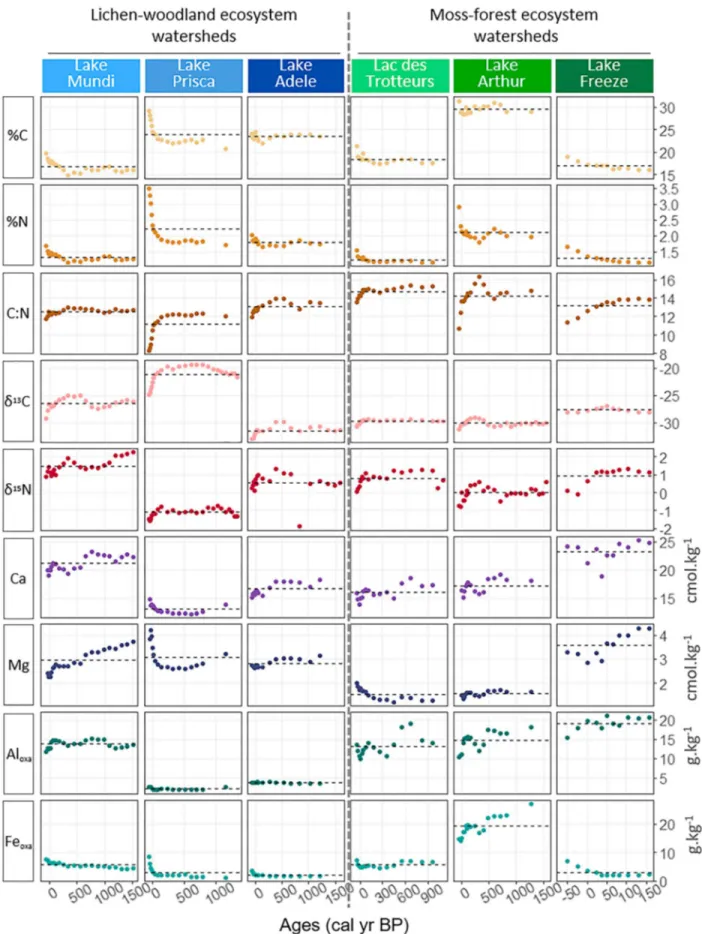
Geochemistry in lake sediments varied between lakes and with age (Figure 1). Variations in geochemical properties appeared to be greatest at the top of the cores (Figure 1), in the youngest sediments, where concentrations of several elements decreased markedly with age in some lakes (e.g., C and N contents, Mg, in the shallowest lakes Lakes Arthur, Prisca, and Freeze). The higher variations in the top sediments may be explained by the sedimentation processes that are occurring at the top core surface, where burying is still incomplete and sediments are less compacted and looser than deeper in the core. Sedimentation pro-cesses could also differ between lakes depending on their shape (size and depth), as noticed by Ferland et al. (2012). Also, OM decomposition and transformation during the sedimentation processes, from degradation in the water column to alteration during early diagenesis, are prejudicial to OM conservation (Bernasconi et al., 1997; Lehmann et al., 2002). However, Ferland et al. (2014) demonstrated that little OM degradation occurred after a few decades after it was deposited. We thus considered that the top sediments could not be reliable enough to perform comparisons of means between sediment and soil geochemistry, or among lakes. We rather decided to deal with sections from which concentrations seemed more stabilized, that is, starting from 0 to 1000 cal yr BP (Figure 1). Thus, the top 5‐ to 10‐cm layer, corresponding to the most liquid parts of the sequences, was discarded from further analysis. The studied forest stands were older than 150 years, thus the ecosystem composition at 0 cal yr BP (1950) should be identical to the composition of the last 65 years. Furthermore, the absence of majorfluctuations in geochemical concentrations from 0 to 1000 cal yr BP supported our hypothesis that no major vegetation change has occurred during this period.
A single geochemical indicator was not identified that distinguish lakes in LW from those in MF watersheds (Figure 1). Nevertheless, some tendencies could be observed, including theδ13C of Lake Prisca and Lake Mundi (LW), which displayed higher average ratios than all MF lakes (mean ranges calculated on the complete depth profile: −21.1 to −29.7 in LW, −27.7 to −30.0 in MF). Also, LW lakes (Adele and Prisca) seemed to hold less Aloxain their sediments than MF lakes did (mean ranges: 2.1 to 13.7 g/kg in LW, 13.2
to 19.1 g/kg in MF).
Looking at single lake profiles (Figure 1), Lake Mundi displayed a biogeochemical profile that resembled more those of lake Freeze and Lac des Trotteurs (both being MF lakes) than those of the other two LW lakes (Prisca and Adele). Lake Mundi was identified as a site surrounded by LW ecosystem due to its low tree density and to the groundcover identified as lichens on satellite images taken before a wildfire that affected the site in 2007. Thefield conditions around this lake were more complex though, with a patchwork of LW on the eastern part of the lake, while the western part contained a denser forest and groundcover remains composed of burnt feathermosses (MF). Lake Mundi should hence be considered as being surrounded by a combination of LW and MF ecosystems. Except for Lake Mundi, Aloxaseemed to be a promising indicator
to differentiate between LW and MF environments.
3.2. Comparisons Between Lakes and Soils Geochemistry in LW and MF
Comparisons between lake sediment and soil geochemistry were performed (Figure 2), and ratios between soil and sediment values are reported in Table S3. Student t tests were performed to compare the geochem-istry of LW and MF sediments (Table S4), but were not always significant, likely due to the low number of sites (n = 6).
Figure 1. Time series profiles of geochemical elements in lakes with age. The horizontal dashed line in each section corresponds to the element mean in the given lake, calculated using all values along the studied core profile (including top sediments) from present to 1500 cal yr BP.
3.2.1. C and N Content
Average C and N concentrations showed little difference between LW and MF sediments (Figure 2 and Table S3), with values close to 21% C and 1.5% N. Yet the C:N ratio had significant higher mean values in MF sediments (14.3 ± 0.8) than in LW sediments (12.6 ± 0.6, p value = 0.037; Figure 2 and Tables S3 and S4).
Studying the geochemistry of lacustrine sediments constitutes a big challenge as numerous factors influence their composition: lake water geochemistry, sediment‐water interface, internal transport and fluxes in sedi-ments, allochthonous inputs from the watershed due to climate, geology, topography and weathering of the watershed, slope, soil, vegetation, and,finally, autochthonous inputs resulting mainly from aquatic biota activities (Meyers, 1997). Losses and transformations of elements from soils to sediment burial can be substantial: for instance, Ferland et al. (2014) showed that the short‐term C accumulation rate in sediment was 10 times lower than the C sinkingflux.
In lakes, the C:N ratio is often used as an indicator of sedimentary OM origin. Low C:N (4–10) suggests that OM is mainly derived from algal material (autochthonous), while C:N values over 20 likely arise from terrestrial vascular plant inputs (allochthonous, Meyers, 1994, 1997, 2003). In our study lakes, the C:N ratios of sediments varied around 12–15 (± 0.5). This does not make it possible to specifically identify the main OM origin, likely from shared allochthonous and autochthonous inputs. Allochthonous inputs still should be Figure 2. Comparison between soil and sediment geochemistry in LW and MF environments. Full symbols for a given element represent the mean values for each site (sediments or soil), while empty symbols represent the mean for each ecosystem type calculated as the overall mean of all MF sites and LW sites, respectively. Blue refers to LW and green to MF. Sed.: Sediments. Oxide:C = (Aloxa+Feoxa):C. Mean values for sediments were calculated by taking samples aged from 0 to (max) 1,000 cal yr BP. Soil means correspond to B horizon values. Statistical tests for soil values were run in Bastianelli et al. (2017). For visualization purposes, y axes do not systematically have the same scale in Sed. and Soils sections.
greater when the vegetation cover is thicker and brings more soil OM from the watershed to the lake (as hypothesized by Huvane & Whitehead, 1996). As previous soil analyses had shown that MF organic layers were thicker and held more C and N than LW soils (Bastianelli et al., 2017), they could infine contribute to bringing more terrestrial inputs of OM to lacustrine sediments in MF watersheds and explain the higher C:N ratios observed in sediments of MF watersheds compared to LW watersheds.
3.2.2. C Accumulation in Sediments
Carbon accumulation rates in the upper sediment portions were calculated by relating C concentration (%C) to the period of time covered by each sample depth, as estimated by radiocarbon dating. Figure 3 shows the mean C accumulation rates in the studied lakes for short‐term accumulation (0–200 cal yr BP) and millennial‐scale accumulation (200–1,000 cal yr BP). We separated both periods because of the variations in sedimentation rates (1:deposition time), which could be attributed to the differences in sedi-ment compression and to the impacts of age models (Figures 3 and S2). The short‐term C accumulation rates were greater than the millennial C accumulation rates (Figure 3). The millennial rates were of the same order of magnitude as the organic C burial rate measured by Chmiel et al. (2016) in another small boreal lake (7.8 ± 1.9 gC·m−2·year) and of the C accumulation rates measured by Ferland et al. (2014) in boreal lake short cores (23–50 cm, 1 to 5 gC·m−2·year). At the millennial scale, we also observed that lakes surrounded by MF ecosystems had higher accumulation rates than lakes surrounded by LW ecosys-tems (p value = 0.021). On the short‐term scale, the variability observed seemed to also depend on the lakes themselves, which is consistent withfindings of Ferland et al. (2014) who concluded that accumulation rates vary depending on the lakes and are correlated with lake morphometry (shape). Small lakes tend to display greater C burial efficiency and hence more efficiently store more C at millennial scales (Cole et al., 2007; Ferland et al., 2014).
Despite the small number of sites, Pearson correlation analyses were attempted to determine whether the morphometry of our lakes could influence the C accumulation rate at either the short‐term or millennial scales (Table S5). In the six study sites, the C accumulation rate was not significantly correlated with any of the studied parameters at the short‐term scale (watershed area, sedimentation rate, water depth, or lake surface area). However, it was positively correlated with the forest stand basal area at the millennial scale (R = 0.98, p = 0.004). Also, the mean deposition rate at the short‐term scale was significantly correlated with the average slope of the watershed (R =−0.89, p = 0.019) and the average basal area of the ecosystem surrounding the lakes (R =−0.84, p = 0.037). Interestingly, the average slope was very strongly correlated with the basal area (R = 0.96, p = 0.003), suggesting that both types of ecosystem (LW and MF) tend to establish themselves on lands with different topography. We suggest that topography of the watersheds could influence local fire regimes and spread processes and partly explain the maintenance of specific ecosystems depending on the relief.
Figure 3. Carbon accumulation rates in lakes at short‐term scale (0–200 cal yr BP) and millennial scale (200–1000 cal yr BP). Accumulation rates were calculated for each sample of sediments according to the formula%C*dwage
s
ð Þ*Swhere %C: carbon content; dw: sample dry weight in gram; ages= median calibrated age of the lower sample− median calibrated age of the sample; S: surface of the corer used to retrieve the sample in m−2. The mean deposition time is given as an indication of sediment compression variations between the two studied time periods.
A study from Li et al. (2015) showed that an important part of the variability of C exports from terrestrial ecosystems into lakes (dissolved inorganic C, dissolved organic C, and total C) could be explained by topo-graphy and vegetation variables. Based on our results, we suggest that the study of C accumulation rates over the long‐term scale could provide interesting perspectives for investigating variations and changes in forest ecosystem density and productivity over time. It could also be used for assessing C stock abilities of boreal lakes depending on future vegetation changes.
3.2.3. Aloxaand FeoxaSpecies
The Aloxaand Feoxa species sediment concentrations showed distinct differences between LW and MF
watersheds as shown in soils (Figure 2). Yet, the dynamics of the variations observed in sediments were opposed to the results obtained in soils: while LW B horizon showed concentrations of Aloxathat were twice
higher than those in MF soils (14.4 ± 1.8 and 6.2 ± 2.9 g/kg, respectively), LW sediments contained on average 2.5 times less Aloxathan MF sediments (6.7 ± 6.6 and 16.1 ± 3.2 g/kg, respectively; Figure 2 and
Table S3).
It should be noted that the illuvial B horizon of LW contains high concentrations of Aloxa, but that this
horizon was much thinner than that of MF soils (Bastianelli et al., 2017). It is thus possible that mineral alteration in LW soils may be intense but operate mainly in a thin soil layer located beneath the lichen mat (Chen et al., 2000). Alternatively, MF soils have a deeper B horizon, indicating that mineral oxidation is happening on a much greater volume of soil particles and could therefore generate more metal oxides for transport to lake sediments.
Once in sediments, oxide species chemically bound to C (such as Aloxaand Feoxa) are very stable and subject
to low degradation (Lalonde et al., 2012), which makes them good candidates for geochemical indicators. Consistently, sediment:soil ratios were different between LW and MF watersheds for Feoxaand Aloxaspecies
(0.4–0.5 in LW for Feoxaand Aloxa, respectively, against 1.6–2.6 in MF; Table S3). Alternatively, it was noted
that the depth of soil profile development was greater in MF (Bastianelli et al., 2017). It is also possible that the more productive MF ecosystem generates more organic acids that in turns enhance mineral oxidation and leaching of organo‐mineral complexes from the watersheds to the lake. The average slope is also likely to play a significant role in matter and fluid transfers.
3.2.4. Exchangeable Cations
Exchangeable cation concentrations (Ca, Mg, and Fe) in sediments showed no specific pattern related to ecosystem type (LW vs MF), while in soils, variations between LW and MF were clearer (Figure 2), especially in FH horizons (humus data not shown; see Bastianelli et al., 2017). These elements may be too mobile to constitute, alone, suitable proxies for estimating the vegetation cover of a watershed in paleoecological investigations. Ratios of certain elements have been reported to be useful to assess vegetation changes that might have occurred in a watershed or to provide information on soil development and on the amount of leakage in a watershed (Huvane & Whitehead, 1996). For instance, Mg and K were reported to be good refer-ences of allochthonous sources and could be used to deduce the autochthonous portion of other elements (Huvane & Whitehead, 1996). Applied to our measured exchangeable cations, we found that their X:K or X:Mg (X: other geochemical elements) ratios did not add conclusive information compared to X noncor-rected values (Figure S3 compared with Figure 2). Again, this is consistent with our hypothesis that no major change in vegetation has occurred during the last 1,000 years at our study sites. Further investigations are needed, on longer timescales, to determine whether exchangeable cations could be used to detect vegetation changes in LW and MF ecosystems.
3.2.5. Isotope Ratios
The carbon isotopic ratio is usually applied to determine whether there has been a change in the dominant vegetation type of a watershed over time or to detect variations in OM inputs (e.g., Bernasconi et al., 1997; Choudhary et al., 2009; Herczeg et al., 2001). Because spruce was the dominant vegetation in our study and uses the C3 photosynthesis pathway, we expected few differences inδ13C between both ecosystem types (MF vs LW), with values in sediment OM around−27‰ (versus −14‰ for plants using the C4 photosynth-esis pathway, for example, nonalgal aquatic plants; Meyers, 1997). Yet lichen species were reported to display higher averageδ13C values than mosses (of ~2.3‰, Lee et al., 2009). As calibration in soils had not been performed previously, we looked at the differences inδ13C andδ15N means in LW and MF B horizons. Interestingly,δ13C significantly differed between LW and MF soils (Figure 2, LW: −25.26‰ ± 0.17; MF:
−25.65‰ ± 0.10). In sediments, tendencies showed that δ13C were on average also lower in MF than in LW
watersheds (LW:−25.81‰ ± 5.48; MF: −29.01‰ ± 1.26), which reflect the isotopic composition of the different ecosystems. The values ofδ13C in sediments were of similar order to that found in other studies (e.g., −26.5 to −27.8‰ in Choudhary et al., 2009). We suggest that rather than focusing on a δ13C threshold value as an indicator of ecosystem type in sediments, we should look atfluctuations along the long sediment sequence to see whether there has been a shift at a certain time.
Regardingδ15N results, no difference in patterns arose in soils nor sediments between both types of ecosys-tems. Sedimentaryδ15N has been assessed as an archive of N cycling that can provide information on terres-trial N availability, OM inputs, environmental, or vegetation changes (Bernasconi et al., 1997; Howard & McLauchlan, 2015; Mayr et al., 2009; McLauchlan et al., 2013). However, like us, Brenner et al. (1999) did notfind any noticeable trend in δ15N variations over time and concluded that there was no correlation betweenδ15N and other studied parameters that determine the trophic state of a lake. They proposed that other drivers might ultimately control theδ15N of OM in sediments. We believe that variations inδ15N in our study lakes are mainly related to disturbance dynamics, particularly fromfire history (see Dunnette et al., 2014). As charcoal analyses revealed no major shift in thefire regime over the last 1,000 years (unpub-lished data), the little variations ofδ15N observed along our sediment sequence could be additional indica-tors of the stability of our ecosystem sites during the last millennium.
3.3. Links Between Geochemical Variables in Sediments and Tree Density of the Watershed
We used the average tree basal area of the surrounding environment measured within a 50‐m perimeter width around each lake to further investigate the relationships between geochemical element Figure 4. Fluctuations of Aloxa,δ13C, and C:N in MF and LW sediments (0–1000 cal yr BP). (a–c) Relationships between the average value of Aloxa,δ13C, and C:N and the average basal area of lake catchments. (d–f) Boxplot of variability of the average value of Aloxa,δ13C, and C:N in each lake catchment.
concentrations in sediments and watershed tree density. Correlation tests were not significant for any of the variables studied (Figures 4a–4c and S4), likely due to the limited number of sites (n = 6). Multiple linear regression models tested using the stepwise method revealed that the best model linking basal area to geochemical variables only included Aloxa. On the other hand, simple t tests performed on mean values of
geochemical elements (considering the 0–1000 cal yr BP period) revealed that only the C:N ratio was signif-icantly different between LW and MF watersheds (Table S4). Similarly, Brenner et al. (1999) also noted that single geochemical proxies in sediments (nutrients, isotope ratios, or pigments) were generally poor indica-tors or predicindica-tors of a lake's trophic status. In particular, they showed that elements such asδ13C could not alone indicate the trophic state of a lake, but rather that they become complementary when linked with other indicators. Thus, while our results should therefore be considered as preliminary due to the lack of sta-tistical significance, they do suggest that further research be conducted to increase the number of sites and data, and to confirm the tendencies found here using sound statistical analyses.
3.4. Stability of Sediment Properties With Depth
The sediment properties stabilized at different depths when comparing LW and MF watersheds (Figures 1 and S5). Elements such asδ13C and Aloxa seemed to fluctuate differently in LW and MF watersheds
(Figures 1 and 4d–4f). We defined and calculated the stability (S) of elements along the sediment depth profile as the mean of value differences between two consecutive samples (i.e., S = mean (value at depth[N]− value at depth[N − 2]), N being the sample mean depth in centimeter). We also defined and calculated the mean absolute difference (MAD) as the mean of absolute differences between each sample value and the mean of all values for each geochemical element. Student t tests on S and MAD showed that Aloxawas significantly (α = 0.05) more stable (less variability) in LW sediments than in MF sediments
(p(S)= 0.020, p(MAD)= 0.043). Conversely,δ13C showed less stability in LW sediments than in MF sediments
(p(S)= 0.049, p(MAD)= 0.051).
We suggest that the differences in stability of Aloxaandδ13C in LW and MF sediments could be linked to the
differences of OM inputs and element transfer from the watersheds of both ecosystem types. OM exports depend on water discharge, watershed size and topography, soil type, hydrologic parameters, and vegetation (Hope et al., 1994; Li et al., 2015). In particular, soil erosion varies with slope, erodibility and depletion abilities of soil material, and climatic factors (Bryan, 2000; Toy et al., 2002). Hence, the increased stability with depth of Aloxain LW sediments could be associated with a certain steadiness of inputs from the LW
watershed, whereas transfers could be more erratic and uneven in MF as a result of their denser, thicker, and richer soil environment and steeper slopes (Bastianelli et al., 2017). As forδ13C, we hypothesized that strong inputs of OM in MF catchments could lead to an almost steady ratio of isotopic C, while even small disturbances in LW catchments could lead to perceptible variations in sediments. However, we found no evidence of correlations betweenδ13C or Aloxaand the sedimentation rates or the C accumulation rates at
our study sites (p > 0.1).
4. Perspectives and Conclusion
Our study showed that while lake sediment C:N ratio, Aloxa, andδ13C differed between MF and LW
ecosys-tems, none of these indicators could be used as a single reliable geomarker or proxy to distinguish between the two terrestrial ecosystem types under study. Yet this exploratory study suggests that lake sediment geo-chemistry could provide useful additional information for studying vegetation dynamics and structure. Of particular importance, we showed that the millennial C accumulation rate was correlated to the tree density of the ecosystems. Ecosystems with different tree densities and productivities hence display differ-ent sedimdiffer-entation dynamics and variations in the stability of certain geochemical elemdiffer-ents along their respective sediment sequences, likely due to variations in OM inputs. A deep understanding of matter transfer, inputs, and transformation, may it concern OM or other geochemical elements, requires a serious focus in upcoming research in order to increase our general knowledge of taphonomicfilters and processes. It could be of tremendous interest to further reconstruct past C stocks from past ecosystem structures. Geochemical proxies could thus help to detect environmental changes over the long timescale. Considering multiple indicators over long sediment profiles along with other markers of environmental changes, such as charcoal and pollen, could increase our capacity to investigate past terrestrial ecosystems composition and state.
References
Appleby, P. G., & Oldfield, F. (1978). The calculation of lead‐210 dates assuming a constant rate of supply of unsupported 210Pb to the sediment. Catena, 5(1), 1–8. https://doi.org/10.1016/S0341‐8162(78)80002‐2
Bastianelli, C., Ali, A. A., Beguin, J., Bergeron, Y., Grondin, P., Hély, C., & Paré, D. (2017). Boreal coniferous forest density leads to significant variations in soil physical and geochemical properties. Biogeosciences, 14(14), 3445–3459. https://doi.org/10.5194/bg‐14‐3445‐2017 Bernasconi, S. M., Barbieri, A., & Simona, M. (1997). Carbon and nitrogen isotope variations in sedimenting organic matter in Lake
Lugano. Limnology and Oceanography, 42(8), 1755–1765.
Bernier, P. Y., Desjardins, R. L., Karimi‐Zindashty, Y., Worth, D., Beaudoin, A., Luo, Y., & Wang, S. (2011). Boreal lichen woodlands: A possible negative feedback to climate change in eastern North America. Agricultural and Forest Meteorology, 151(4), 521–528. https://doi.org/10.1016/j.agrformet.2010.12.013
Birks, H. H., & Birks, H. J. B. (2006). Multi‐proxy studies in palaeolimnology. Vegetation History and Archaeobotany, 15(4), 235–251. https://doi.org/10.1007/s00334‐006‐0066‐6
Blaauw, M., & Christen, J. A. (2011). Flexible paleoclimate age‐depth models using an autoregressive gamma process. Bayesian Analysis, 6(3), 457–474.
Blaauw, M., & Christen, J. A. (2013). Bacon Manual e v2. 2.
Blarquez, O., Finsinger, W., & Carcaillet, C. (2013). Assessing paleo‐biodiversity using low proxy influx. PLoS ONE, 8(6), e65852. https://doi.org/10.1371/journal.pone.0065852
Brenner, M., Whitmore, T. J., Curtis, J. H., Hodell, D. A., & Schelske, C. L. (1999). Stable isotope (δ13C and δ15N) signatures of sedimented organic matter as indicators of historic lake trophic state. Journal of Paleolimnology, 22(2), 205–221.
Broström, A., Nielsen, A. B., Gaillard, M.‐J., Hjelle, K., Mazier, F., Binney, H., et al. (2008). Pollen productivity estimates of key European plant taxa for quantitative reconstruction of past vegetation: A review. Vegetation History and Archaeobotany, 17(5), 461–478. https://doi. org/10.1007/s00334‐008‐0148‐8
Bryan, R. B. (2000). Soil erodibility and processes of water erosion on hillslope. Geomorphology, 32(3), 385–415. https://doi.org/10.1016/ S0169‐555X(99)00105‐1
Castañeda, I. S., & Schouten, S. (2011). A review of molecular organic proxies for examining modern and ancient lacustrine environments. Quaternary Science Reviews, 30(21), 2851–2891. https://doi.org/10.1016/j.quascirev.2011.07.009
Chen, J., Blume, H.‐P., & Beyer, L. (2000). Weathering of rocks induced by lichen colonization—A review. Catena, 39(2), 121–146. https://doi.org/10.1016/S0341‐8162(99)00085‐5
Chmiel, H. E., Kokic, J., Denfeld, B. A., Einarsdóttir, K., Wallin, M. B., Koehler, B., et al. (2016). The role of sediments in the carbon budget of a small boreal lake. Limnology and Oceanography, 61(5), 1814–1825. https://doi.org/10.1002/lno.10336
Choudhary, P., Routh, J., Chakrapani, G. J., & Kumar, B. (2009). Biogeochemical records of paleoenvironmental changes in Nainital Lake, Kumaun Himalayas, India. Journal of Paleolimnology, 42(4), 571–586.
Cole, J. J., Prairie, Y. T., Caraco, N. F., McDowell, W. H., Tranvik, L. J., Striegl, R. G., et al. (2007). Plumbing the global carbon cycle: Integrating inland waters into the terrestrial carbon budget. Ecosystems, 10(1), 172–185. https://doi.org/10.1007/s10021‐006‐9013‐8 Dunnette, P. V., Higuera, P. E., McLauchlan, K. K., Derr, K. M., Briles, C. E., & Keefe, M. H. (2014). Biogeochemical impacts of wildfires
over four millennia in a Rocky Mountain subalpine watershed. New Phytologist, 203(3), 900–912. https://doi.org/10.1111/nph.12828 Ferland, M., Giorgio, P. A., Teodoru, C. R., & Prairie, Y. T. (2012). Long‐term C accumulation and total C stocks in boreal lakes in northern
Québec. Global Biogeochemical Cycles, 26, Gb0e04. https://doi.org/10.1029/2011GB004241
Ferland, M., Prairie, Y. T., Teodoru, C., & Giorgio, P. A. (2014). Linking organic carbon sedimentation, burial efficiency, and long‐term accumulation in boreal lakes. Journal of Geophysical Research: Biogeosciences, 119, 836–847. https://doi.org/10.1002/2013JG002345 Ficken, K. J., Wooller, M. J., Swain, D. L., Street‐Perrott, F. A., & Eglinton, G. (2002). Reconstruction of a subalpine grass‐dominated ecosystem, Lake Rutundu, Mount Kenya: A novel multi‐proxy approach. Palaeogeography, Palaeoclimatology, Palaeoecology, 177(1), 137–149. https://doi.org/10.1016/S0031‐0182(01)00356‐X
Gaillard, M.‐J. (2007). Pollen methods and studies: Archaeological applications. In S. A. Elias, & C. Mock (Eds.), Encyclopedia of Quaternary Science, (Second ed.pp. 880–904). Amsterdam: Elsevier.
Gauthier, S., Bernier, P., Kuuluvainen, T., Shvidenko, A. Z., & Schepaschenko, D. G. (2015). Boreal forest health and global change. Science, 349(6250), 819–822. https://doi.org/10.1126/science.aaa9092
Girard, F., Payette, S., & Gagnon, R. (2008). Rapid expansion of lichen woodlands within the closed‐crown boreal forest zone over the last 50 years caused by stand disturbances in eastern Canada. Journal of Biogeography, 35(3), 529–537.
Girard, F., Payette, S., & Gagnon, R. (2009). Origin of the lichen–spruce woodland in the closed‐crown forest zone of eastern Canada. Global Ecology and Biogeography, 18(3), 291–303.
Herczeg, A. L., Smith, A. K., & Dighton, J. C. (2001). A 120 year record of changes in nitrogen and carbon cycling in Lake Alexandrina, South Australia: C:N,δ15N and δ13C in sediments. Applied Geochemistry, 16(1), 73–84. https://doi.org/10.1016/S0883‐2927(00)00016‐0 Hope, D., Billett, M., & Cresser, M. (1994). A review of the export of carbon in river water: Fluxes and processes. Environmental Pollution,
84(3), 301–324.
Howard, I., & McLauchlan, K. K. (2015). Spatiotemporal analysis of nitrogen cycling in a mixed coniferous forest of the northern United States. Biogeosciences, 12(13), 3941–3952. https://doi.org/10.5194/bg‐12‐3941‐2015
Huvane, J., & Whitehead, D. (1996). The paleolimnology of North Pond: Watershed‐lake interactions. Journal of Paleolimnology, 16(3), 323–354.
Jasinski, J. P., & Payette, S. (2005). The creation of alternative stable states in the southern boreal forest, Quebec, Canada. Ecological Monographs, 75(4), 561–583.
Johnson, E. A. (1992). Fire and vegetation dynamics: studies from the North American boreal forest. New York: Cambridge University Press. Lalonde, K., Mucci, A., Ouellet, A., & Gélinas, Y. (2012). Preservation of organic matter in sediments promoted by iron. Nature,
483(7388), 198.
Lamb, H. F. (1984). Modern pollen spectra from Labrador and their use in reconstructing Holocene vegetational history. The Journal of Ecology, 37–59.
Lee, Y. I., Lim, H. S., & Yoon, H. I. (2009). Carbon and nitrogen isotope composition of vegetation on King George Island, maritime Antarctic. Polar Biology, 32(11), 1607–1615.
Lehmann, M. F., Bernasconi, S. M., Barbieri, A., & McKenzie, J. A. (2002). Preservation of organic matter and alteration of its carbon and nitrogen isotope composition during simulated and in situ early sedimentary diagenesis. Geochimica et Cosmochimica Acta, 66(20), 3573–3584. https://doi.org/10.1016/S0016‐7037(02)00968‐7
Acknowledgments
This research was funded by the Natural Sciences and Engineering Research Council of Canada (NSERC), the European FP7‐PEOPLE‐2013‐ IRSES‐NEWFOREST project, the Institut écologie et environnement of the Centre national de la recherche scientifique (CNRS‐InEE), the École Pratique des Hautes Études, and the Université de Montpellier (France) through the International Research Group on Cold Forests (GDRI Forêts Froides, France) and the Institut Universitaire de France (IUF). The Ph. D. thesis of Carole Bastianelli was sup-ported by AgroParisTech. The authors are grateful to Serge Rousseau for car-rying out laboratory experiments; to Lise Rancourt (INRS), Jean‐Francois Hélie (Geotop), and Guillaume Labrecque (CEN) for their involvement in datings and isotopic ratio measure-ments and for providing useful details about the methods; to David Gervais, Sébastien Dagnault, Benoît Brossier, Raynald Julien, Olivier Blarquez, Evrard Kouadio, Benoît Gaudreau, and Samuel Alleaume for their help with field work; to Julien Béguin for his helpful advice in statistical analyses; and to Danielle Charron for her administrative support. The authors also thank Véronique Poirier and Pierre Grondin from the Direction de la recherche forestière of the Ministère des Forêts, de la Faune et des Parcs du Québec (MFFP) for providing helpful geographical and spatial information and Pierre Clouâtre for technicalfield support. Special thanks to Laure Paradis for her help in spatial and geo-graphical analyses to determine the topography of the watersheds, to Sebastien Joannin for very helpful comments and inputs during the manuscript preparation process, and to Isabelle Lamarre and Paul Jasinski for their help in proofreading this paper. Finally, the authors are particularly grateful to the anonymous reviewers who provided relevant, helpful, and constructive comments that helped improving this paper. The raw data compiled for this study are available at https://doi.org/10.13140/
RG.2.2.12565.52965 and https://doi. org/10.13140/RG.2.2.30348.00648.
Li, M., Giorgio, P. A., Parkes, A. H., & Prairie, Y. T. (2015). The relative influence of topography and land cover on inorganic and organic carbon exports from catchments in southern Quebec, Canada. Journal of Geophysical Research: Biogeosciences, 120, 2562–2578. https:// doi.org/10.1002/2015JG003073
Mayr, C., Lücke, A., Maidana, N. I., Wille, M., Haberzettl, T., Corbella, H., et al. (2009). Isotopicfingerprints on lacustrine organic matter from Laguna Potrok Aike (southern Patagonia, Argentina) reflect environmental changes during the last 16,000 years. Journal of Paleolimnology, 42(1), 81–102. https://doi.org/10.1007/s10933‐008‐9249‐8
McLauchlan, K. K., Williams, J. J., Craine, J. M., & Jeffers, E. S. (2013). Changes in global nitrogen cycling during the Holocene epoch. Nature, 495(7441), 352–355. https://doi.org/10.1038/nature11916
Meyers, P. A. (1994). Preservation of elemental and isotopic source identification of sedimentary organic matter. Chemical Geology, 114(3–4), 289–302.
Meyers, P. A. (1997). Organic geochemical proxies of paleoceanographic, paleolimnologic, and paleoclimatic processes. Organic Geochemistry, 27(5–6), 213–250.
Meyers, P. A. (2003). Applications of organic geochemistry to paleolimnological reconstructions: A summary of examples from the Laurentian Great Lakes. Organic Geochemistry, 34(2), 261–289.
Mourier, B., Poulenard, J., Carcaillet, C., & Williamson, D. (2010). Soil evolution and subalpine ecosystem changes in the French Alps inferred from geochemical analysis of lacustrine sediments. Journal of Paleolimnology, 44(2), 571–587. https://doi.org/10.1007/s10933‐ 010‐9438‐0
Mustaphi, C. J. C., Davis, E. L., Perreault, J. T., & Pisaric, M. F. (2015). Spatial variability of recent macroscopic charcoal deposition in a small montane lake and implications for reconstruction of watershed‐scale fire regimes. Journal of Paleolimnology, 54(1), 71–86. Overpeck, J. T., Webb, R. S., & Webb, T. (1992). Mapping eastern North American vegetation change of the past 18 ka: No‐analogs and the
future. Geology, 20(12), 1071–1074. https://doi.org/10.1130/0091‐7613(1992)020<1071:MENAVC>2.3.CO;2
Payette, S. (1992). Fire as a controlling process in the North American boreal forest. In A Systems Analysis of the Global Boreal Forest (pp. 144–169). New York: Cambridge University Press.
Payette, S., & Delwaide, A. (2018). Tamm review: The North‐American lichen woodland. Forest Ecology and Management, 417, 167–183. https://doi.org/10.1016/j.foreco.2018.02.043
R Core Team (2013). R: A language and environment for statistical computing.
Rapanoela, R., Raulier, F., & Gauthier, S. (2016). Regional instability in the abundance of open stands in the boreal forest of eastern Canada. Forests, 7(5), 103. https://doi.org/10.3390/f7050103
Reimer, P. J., Bard, E., Bayliss, A., Beck, J. W., Blackwell, P. G., Ramsey, C. B., et al. (2013). IntCal13 and Marine13 radiocarbon age cali-bration curves 0–50,000 years cal BP. Radiocarbon, 55(04), 1869–1887. https://doi.org/10.2458/azu_js_rc.55.16947
Remy, C. C., Hély, C., Blarquez, O., Magnan, G., Bergeron, Y., Lavoie, M., & Ali, A. A. (2017). Different regional climatic drivers of Holocene large wildfires in boreal forests of northeastern America. Environmental Research Letters, 12(3), 035005. https://doi.org/ 10.1088/1748‐9326/aa5aff
Richard, P. (1975). Histoire postglaciaire de la végétation dans la partie centrale du Parc des Laurentides. Naturaliste Canadien: Québec. Richard, P. J., & Grondin, P. (2009). Histoire postglaciaire de la végétation. In Manuel de Foresterie, (2e Éd ed. pp. 170–176). Québec:
Éditions MultiMondes.
Richard, P. (1979). Contribution à l'histoire postglaciaire de la végétation au nord‐est de la Jamésie, Nouveau‐Québec. Géographie Physique et Quaternaire, 33(1), 93. https://doi.org/10.7202/1000324ar
Toy, T. J., Foster, G. R., & Renard, K. G. (2002). Soil erosion: Processes, prediction, measurement, and control. New York: John Wiley & Sons. von Wachenfeldt, E., & Tranvik, L. J. (2008). Sedimentation in boreal lakes—The role of flocculation of allochthonous dissolved organic
matter in the water column. Ecosystems, 11(5), 803–814. https://doi.org/10.1007/s10021‐008‐9162‐z
Weber, M. G., & Flannigan, M. D. (1997). Canadian boreal forest ecosystem structure and function in a changing climate: Impact onfire regimes. Environmental Reviews, 5(3–4), 145–166. https://doi.org/10.1139/a97‐008