Application of machine learning : automated trading informed by event driven data

Application of Machine Learning: Automated

Trading Informed by Event Driven Data

by

Jason W. Leung

Submitted to the Department of Electrical Engineering and Computer

Science

in partial fulfillment of the requirements for the degree of

Master of Engineering in Electical Engineering and Computer Science

at the

MASSACHUSETTS INSTITUTE OF TECHNOLOGY

June 2016

c

○2016 Jason W. Leung, All rights reserved.

The author hereby grants to M.I.T. permission to reproduce and to distribute publicly paper and electronic copies of this thesis document in whole and in part in any medium

now known or hereafter created

.

Author . . . .

Department of Electrical Engineering and Computer Science

May 6, 2016

Certified by . . . .

Jacob K. White

Cecil H. Green Professor; Professor of Electrical Engineering and

Computer Science

Thesis Supervisor

Accepted by . . . .

Dr. Christopher J. Terman

Chairman, Master of Engineering Thesis Committee

Application of Machine Learning: Automated Trading

Informed by Event Driven Data

by

Jason W. Leung

Submitted to the Department of Electrical Engineering and Computer Science on May 6, 2016, in partial fulfillment of the

requirements for the degree of

Master of Engineering in Electical Engineering and Computer Science

Abstract

Models of stock price prediction have traditionally used technical indicators alone to generate trading signals. In this paper, we build trading strategies by applying machine-learning techniques to both technical analysis indicators and market senti-ment data. The resulting prediction models can be employed as an artificial trader used to trade on any given stock exchange. The performance of the model is evaluated using the S&P500 index.

Thesis Supervisor: Jacob K. White

Title: Cecil H. Green Professor; Professor of Electrical Engineering and Computer Science

Acknowledgments

I would like to express my gratitude to my supervisor, Professor Jacob K. White of the Electrical Engineering and Computer Science department at MIT. The door to Professor White’s office was always open whenever I was in need of help or had questions about my research or writing. He consistently allowed this paper to be my own work, but steered me in the right direction whenever he thought I needed it.

A very special thanks goes out to Professor Paul Asquith of the Finance depart-ment at MIT Sloan School of Managedepart-ment. Professor Asquith is the one professor who has truly made a difference in my life. It was under his tutelage that I developed an interest in financial markets and began to consider the ways that my computer science background can be directed in this area. He provided me with direction and became more of a mentor and friend, than a professor. I doubt that I will ever be able to convey my appreciation fully, but I owe him my eternal gratitude.

I would also like to thank my family for the support they provided me throughout my entire life. I will never forget that it is my parents’ sacrifices that made my education possible.

Finally, I must acknowledge Mia Zhang, without whose love and encouragement I would not have finished this thesis.

Contents

1 Introduction 13

1.1 Outline of this Paper . . . 15

2 Literature Review 17 2.1 Efficient Markets . . . 17

2.2 Previous Research . . . 19

3 Machine Learning Algorithms 23 3.1 Neural Network . . . 23

3.2 Random Forest . . . 26

3.3 Support Vector Machines . . . 29

4 Data Preparation 35 4.1 Feature Generation . . . 35

5 Trading System Results 39 5.1 Neural Network . . . 39 5.1.1 Parameter Optimization . . . 39 5.1.2 Out-of-sample Results . . . 40 5.2 Random Forest . . . 43 5.2.1 Parameter Optimization . . . 44 5.2.2 Out-of-sample Results . . . 46

5.3 Support Vector Machines . . . 49

5.3.2 Out-of-sample Results . . . 49 5.4 Comparing the Machine Learning Models . . . 50

6 Closing Remarks 53

6.1 Conclusion . . . 53 6.2 Further Work . . . 54

List of Figures

3-1 Two layer neural network . . . 25 3-2 Simple decision tree for two dimensional feature space . . . 26 3-3 Fraction of training samples that belong to all trees in random forest 28 3-4 Simple example showing soft SVM’s decision boundary . . . 30 3-5 Visual effect of varying Gaussian kernel SVM parameters . . . 32 3-6 Validation accuracy from varying 𝐶 and 𝛾 parameters in SVM with

Gaussian kernel . . . 33

5-1 Cross-entropy error from varying 𝑀 and 𝛾 parameters in NN . . . 41 5-2 Convergence of neural network on training, validation and test data . 42 5-3 Cumulative return performance of optimized Neural Network model

compared to simple buy-and-hold strategy . . . 43 5-4 Classification error for out-of-bag and test data as 𝑀 is increased . . 45 5-5 _{Out-of-bag feature importance for the feature set x ∈ R}214 . . . 46 5-6 _{Out-of-bag classification error for reduced feature set x ∈ R}20 _{. . . . 47}

5-7 Cumulative return performance of optimized Random Forest model compared to simple buy-and-hold strategy . . . 48 5-8 Cross-validation error from varying 𝐶 and 𝜎 parameters in SVM model 50 5-9 Cumulative return performance of optimized SVM model compared to

List of Tables

5.1 Comparing the performance for various values of 𝜖 . . . 40 5.2 Top 10 features in random forest ordered by decreasing feature

Impor-tance . . . 45 5.3 Performance comparison of the three models against a simple

buy-and-hold strategy . . . 50

A.1 A description of all technical analysis features used . . . 57 A.2 A description of all market sentiment features used . . . 59

Chapter 1

Introduction

Predicting the future of stock prices has been the subject of study for both individuals and financial firms for many years. The monetary motivation behind the predictive value of buying and selling stocks at profitable positions is a key driver of this research. Traditionally, methods used to evaluate stocks and generate trade signals fall into two main categories - fundamental analysis and technical analysis. More recently, sentiment analysis has also contributed to generate trade signals.

Fundamental analysis involves studying a company’s fundamental information such as the income statement, balance sheet, cash-flow statement, news release and company policies. On the other hand, technical analysis evaluates the underlying movement of the stock price and traded volume. Subscribers of this methodology believe that all available information, including that of a company’s fundamentals, is already contained within the price history. While technical analysis used to be qualitative in nature - with the goal of identifying regularities by extracting patterns from noisy data and visually examining graphs of stock price movements, modern breakthroughs in technology and machine learning algorithms have transformed this methodology into a more quantitative tool. Studies show that 80% to 90% of polled professionals and individual investors rely on at least some form of technical

analy-sis [44] [29] [27]. Sentiment analyanaly-sis, which involves quantifying the market reaction to particular news events or earnings reports has also recently shown predictive value. A combination of both technical analysis indicators and market sentiment indicators are used in this paper.

The scarcity of published working trading strategies in this area is often attributed to the lack of incentive to publish profitable systems. With large monetary rewards from using or selling such systems, there is an inherent negative bias in academic lit-erature. Some suggest that reason for the lack of published working models is due to the difficulty of publishing empirical results that are often almost statistically insignif-icant, resulting in a possible “file drawer” bias in published studies [45]. Traditional forms of stock market prediction are also rarely consistently profitable, as they may be unable to adapt to the changing market conditions.

Indeed, markets do not remain stable and indicators that have strong predictive value over one period may cease to generate excess returns as soon as market con-ditions change. Two measures have been proposed to counter this evolving market behavior. First, some trading systems are based on genetic algorithms that transform the indicators that are used as attributes over time [6] [28]. Second, more commonly, the data set is fit to nonlinear models using machine learning algorithms such as Artificial Neural Networks [10].

In this paper, we adopt the latter approach and examine the accuracy and perfor-mance of various machine learning classification algorithms, using both quantitative technical and sentiment data as features, in creating a trading strategy that outper-forms the market. We implement feature generation, cross-validation to find optimal parameters and regularizing parameters to avoid over-fitting. By aggregating a 10-year period of S&P500 market data, we train and optimize different models to predict stock price movements. We then conduct out of sample tests to examine the prof-itability of the trading systems compared to a simple buy-and-hold strategy.

1.1

Outline of this Paper

The following provides an outline of this paper:

∙ Chapter 2 This chapter conducts a literature overview of research involving machine learning methods applied to stock price prediction.

∙ Chapter 3 This chapter examines three machine learning techniques used for the classification problem, detailing their mathematical formulation.

∙ Chapter 4 This chapter describes how we generated and prepared the technical and sentiment indicators to be used for machine learning.

∙ Chapter 5 This chapter details the accuracy and performance of the three machine learning techniques on the training, validation and testing data sets. ∙ Chapter 6 This chapter concludes our findings and proposes further research

Chapter 2

Literature Review

This section begins with a background to efficient markets and then gives a brief review of previous empirical studies that use machine learning algorithms to construct trading strategies.

2.1

Efficient Markets

One of the strongest oppositions to the existence of profitable trading strategies is founded on the ideas of Efficient Market Hypothesis (EMH). Since EMH implies that our search for continuously profitably trading strategies is futile, we first give an overview of EMH and then show the empirical results that contradict this theory.

EMH states that the current market price reflects the assimilation of all the in-formation available [13]. That is, its proponents argue that since the stocks always trade at their fair value on stock exchanges, it is impossible to outperform the overall market through expert stock selection or market timing. Any new information is quickly integrated into the market price. Fama formalized the concept of efficient

markets in 1970 by expressing the non-predictability of market prices:

𝐸(˜𝑝𝑗,𝑡+1|Φ𝑡) = [1 + 𝐸(˜𝑟𝑗,𝑡+1|Φ𝑡)]𝑝𝑗, 𝑡 (2.1)

,where 𝑝𝑗,𝑡 is the price of security 𝑗 at time 𝑡, 𝑟𝑗,𝑡+1 is the one-period percentage

return, and Φ𝑡 is the information reflected at time 𝑡. Based on this expectation

expression, Fama argues that there is no possibility of finding excess market returns via market timing based solely on information in Φ𝑡, hence dispelling the possibility

of trading strategies based on technical indicators.

On the other hand, despite the theoretically sound nature of EMH, research over the last 30 years has shown that several assumptions made in EMH may be unrealis-tic. First, a fundamental assumption is that investors behave rationally, or that the deviations of the many irrational investors cancel out. However, some research has shown that investors are not strictly rational [41], or devoid of biases [20]. Indeed, people with a conservatism bias tend to underweight new information. Moreover, experiments have shown that these biases tend to be systematic and that deviations do not cancel each other out [21]. This leads to over- and under-reaction to news events.

From the 1990s, literature has seen the growing decline of the EMH and the emergence of behavioral finance. Behavioral finance views the market as an aggregate of human actions filled with imperfect and inefficient decisions. Under this theory, the financial markets are a reflection of human desires, goals, motivations, errors and overconfidence [40]. An alternative to EMH that has grown traction is the idea of the Adaptive Market Hypothesis, which posits that profit opportunities from inefficiencies exist in finance markets but are eroded away as the knowledge of the efficiency spreads throughout the public and the public capitalizes on the opportunities [26] [32]. By this view of financial markets, many have built evolutionary and/or non-linear models and demonstrated that excess returns can be attained on out-of-sample data.

2.2

Previous Research

Because of their ability to model nonlinear relationships without pre-specification during the modeling process, neural networks (NNs) have become a popular method in financial time-series forecasting. NNs also offer huge flexibility in the type of architecture of the model, in terms of number of hidden nodes and layers. Indeed, Pekkaya and Hamzacebi compare the results from using a linear regression versus a NN model to forecast macro variables and show that the NN gives much better results [35].

Many studies have used NNs and shown promising results in the financial markets. Grudnitski and Osburn implemented NNs to forecast S&P500 and Gold futures price directions and found they were able to correctly prediction the direction of monthly price changes 75% and 61% respectively [15]. Another study showed that a NN-based model leads to higher arbitrage profits compared to cost of carry models [47]. Phua, Ming and Lin implement a NN using Singapore’s stock market index and show a forecasting accuracy of 81% [36]. Similarly, NN models applied to weekly forecasting of Germany’s FAZ index find favorable predictive results compared to conventional statistical approaches [14].

More recently, NNs have been augmented or adapted to improve performance on financial time series forecasting. Shaoo et al. show that cascaded functional link artificial neural networks (CFLANN) perform the best in FX markets [39]. Egrioglu et al. introduce a new method based on feed forward artificial neural networks to analyze multivariate high order fuzzy time series forecasting models [12]. Liao and Wang used a stochastic time effective neural network model to show predictive results on the global stock indices [25]. Bildirici and Ersin combined NNs with ARCH/GARCH and other volatility based models to produce a model that out performed ANNs or GARCH based models alone [4]. Moreover, Yudong and Lenan used bactrial chemotaxis optimization (BCO) and back-propagation NN on S&P500 index and conclude that their hybrid model (IBCO-BP) offers less computational complexity,

better prediction accuracy and less training time [48].

Another popular machine learning classification technique that does not require any domain knowledge or parameter setting is the decision tree. It also often offers a better visually interpretable model compared to NN, as the nodes in the tree can be easily understood. The simplest type of decision tree model is the classification and regression tree (CART). Sorensen et al. show that CART decision trees perform better than single-factor models based on the same variables in picking stock portfolios [42]. Wang and Chan use a two-layer bias decision tree to predict the daily stock prices of Microsoft, Intel and IBM, finding excess returns compared to a buy-and-hold method [43]. Another study found that a boosted alternating decision tree with expert weighing generated abnormal returns for the S&P500 index during the test period [11]. To improve accuracy, some studies used the random forest algorithm for classification, which will be further discussed in chapter 4. Namely, Booth et al. show that a regency-weighted ensemble of random forests produce superior results when analyzed on a large sample of stocks from the DAX in terms of both profitability and prediction accuracy compared with other ensemble techniques [7]. Similarly, a gradient boosted random forest model applied to Singapore’s stock market was able to generate excess returns compared with a buy-and-hold strategy [37]. Some recent research combine decision tree analysis with evolutionary algorithms to allow the model to adapt to changing market conditions. Hsu et al. present constraint-based evolutionary classification trees (CECT) and show strong predictability of a company’s financial performance [16].

Support Vector Machines (SVM) are also often used in prediction market behav-iors. Huang et al. compare SVM with other classification methods (random Walk, linear discriminant analysis, quadratic discriminant analysis and elman backpropa-gation neural networks) and finds that SVM performs the best in forecasting weekly movements of the Nikkei 225 index [17]. Similarly, Kim compares SVM with NN and case-based reasoning (CBR) and finds that SVM outperforms both in forecasting the daily direction of change in the Korea composite stock price index (KOSPI) [23].

Likewise, Yang et al. use a margin-varying Support Vector Regression model and show empirical results that have good predictive value for the Hang Seng Index [46]. Nair et al. propose a system that is a genetic algorithm optimized decision tree-support vector machine hybrid and validate its performance on the BSE-Sensex and found that its predictive accuracy is better than that of both a NN and Naive bayes based model [31].

While some studies have tried to compare various machine learning algorithms against each other, the results have been inconsistent. Patel et al. compares four prediction models, NN, SVM, random forest and naive-Bayes and find that over a ten year period of various indices, the random forest model performed the best [34]. However, Ou and Wang examine the performance of ten machine learning classifica-tion techniques on the Hang Sen Index and found that the SVM outperformed the other models [33]. Kara et al. compared the performance of NN versus SVM on the daily Instabul Stock Exchange National 100 Index and found that the average performance of the NN model (75.74%) was significantly better than that of the SVM model (71.52%) [22].

Chapter 3

Machine Learning Algorithms

This chapter reviews the machine learning algorithms used to generate trading sys-tems in chapter 5. We summarize the general concepts behind each algorithm and detail the free parameters that are determined via cross-validation.

All three algorithms explored are used for a supervised learning classification prob-lem where we are given data, {𝑥𝑖_,𝑦𝑖_{} for 𝑖 = 1, 2..., 𝑁 . The input variable 𝑥}𝑖_=𝑥

1, ..., 𝑥𝐷

is 𝐷 dimensional, i.e. 𝑥𝑖 ⊂ 𝜒.The variable 𝑦𝑖 _{⊂ 𝛾 indicates the class that the samples}

belongs to. The goal is to come up with a prediction rule ℎ : 𝜒 → 𝛾.

3.1

Neural Network

Neural Networks extend the general linear classification model by allowing the model to learn the basis functions from the data. Specifically, in a general classification model: 𝑦(x,w) = 𝑓 ( 𝑀 ∑︁ 𝑗=1 𝑤𝑗𝜑𝑗(𝑥))

,we have that 𝑓 () is a nonlinear activation function, and the coefficients 𝑤𝑗 are

ad-justed during training. Neural networks give added modeling power by allowing the basis functions (features), 𝜑𝑗(𝑥), to be learned during training too [5].

Specifically, we define 𝜑𝑗(𝑥) = 𝑔(𝑎𝑗) 𝑎𝑗 = 𝑑 ∑︁ 𝑖=1 𝑤1_𝑗𝑖𝑥𝑖+ 𝑤1𝑗0

so each layer 𝑙 of features is:

𝑧_𝑗𝑙 = 𝑔(

𝑖=𝑑

∑︁

𝑖=0

𝑤𝑙_𝑗𝑖𝑧_𝑖𝑙−1)

In this paper, we use a 2-layer regularized neural network with the number of samples, 𝑁 , the number of classes = 𝐾 and the sigmoid activation function for both the hidden and output:

𝑔(𝑧) = 1 1 + 𝑒−𝑧

Such that our expression for the 2-layer network is:

𝑓𝑘(𝑥, 𝑤) = 𝑔( 𝑗=𝑀 ∑︁ 𝑗=0 𝑤_𝑘𝑗2 𝑔( 𝑖=𝑑 ∑︁ 𝑖=0 𝑤_𝑗𝑖1𝑥𝑖))))

By backwards propogation, we train our parameters 𝑤 = {𝑤1, 𝑤2} and output class ℎ𝑘(𝑥, 𝑤) by choosing the max of {𝑦1, ..., 𝑦𝑘}. With this choice of ℎ𝑘(𝑥, 𝑤), we

have the cost function, with regularization: 𝑙(𝑤) = 𝑁 ∑︁ 𝑖=1 𝐾 ∑︁ 𝑘=1 (−𝑦𝑖_𝑘log(ℎ𝑘(𝑤𝑖, 𝑤)) − (1 − 𝑦𝑖)log(1 − (ℎ𝑘(𝑥𝑖, 𝑤))) 𝐽 (𝑤) = 𝑙(𝑤) + 𝜆(‖𝑤1‖2 𝐹 + ‖𝑤 2_‖2 𝐹)

Figure 3-1: Figure of two-layer neural network [5]

Figure 3-1 shows the structure of such a 2-layer neural network.

Training the network corresponds to a non-convex optimization problem, and var-ious heuristics are employed. While a more thorough analysis of the varvar-ious heuristics that exist is outside the scope of this paper, we mention that some of popular methods include greatest descent and conjugate gradient.

In chapter 5, cross validation is used to determine the parameters 𝑀 , number of nodes in the hidden layer, 𝑤 = {𝑤1_{, 𝑤}2_{}, which are the weights in the model and 𝜆,}

which is the regularization parameter.

3.2

Random Forest

Random Forest is an extension of decision tree methods, and, similar to NN, attempts to learn the basis functions 𝜑𝑗() from the dataset. To understand Random Forest, we

first explain the basics of decision trees.

Figure 3-2: Figure of simple decision tree for two dimensional feature space, split into 5 regions [30]

In particular, classification and regression trees (CART) models use a series of nodes to determine the value of some input 𝑥. Each node creates axis parallel splits to partition the entire R𝐷 _{space into different regions [30]. Figure 3-2 shows a simple}

example in which a simple regression tree is formed in a two dimensional feature space. We can write the model in the form:

𝑦(x) = 𝑓 ( 𝐾 ∑︁ 𝑘=1 𝑤𝑘𝜑(x,v𝑘)) =𝑓 ( 𝐾 ∑︁ 𝑘=1 𝑤𝑘I(x∈ 𝑅𝑘))

function 𝑓 () depends on whether a classification or regression tree is needed.

While finding the optimal partitioning of the data is NP-complete [18], it is com-mon practice to compute a locally optimal solution using a greedy procedure. The greedy method is used by CART [8], C4.5 [19] and ID3 [38]. The splitting function chooses the best feature, and best value for that feature by minimizing the costs with respect to the split:

(𝑗*, 𝑡*) = arg min_{𝑗∈{1,...,𝐷}}min𝑡∈𝑇𝑗cost({x𝑖, 𝑦𝑖 : 𝑥𝑖𝑗 ≤ 𝑡}) + cost({x𝑖, 𝑦𝑖 : 𝑥𝑖𝑗 > 𝑡})

, where 𝑇𝑗 are the possible thresholds for feature 𝑗.

In this paper, we use the entropy classification cost, which maximizes the infor-mation gain between test 𝑋𝑗 < 𝑡 and class label 𝑌 . The entropy is defined as:

H(ˆ𝜋) = − 𝐶 ∑︁ 𝑐=1 ˆ 𝜋𝑐logˆ𝜋𝑐

CART models are easy to interpret, since the tree can be understood as a series of logic rules, “If 𝑥1 < ..., then...”, and they perform automatic variable selection, scale

well and are insensitive to monotone transformations of inputs. However, they do not have high predictive accuracy due to the greedy nature of tree construction. Indeed, small changes to the input data can have large effects on the structure of the tree, i.e. the trees produced are unstable [30].

To remedy this problem, the random forest technique [9] extends decision trees in two ways. First, to reduce the variance of the estimates, it uses a technique called bagging (bootstrap aggregating) by training 𝑀 different trees and computeing the ensemble:

𝑦(𝑥) = 𝑀 ∑︁ 𝑚=1 1 𝑀𝑦𝑚(𝑥)

,where 𝑦𝑚 is the 𝑚’th tree. Secondly, random forest tries to decorrelate the base

learners by learning trees based on a randomly chosen subset of input variables and a randomly chosen subset of data cases [30]. This is shown in Figure 3-3, illustrating, for a typical graph, the fraction of samples that belong to all trees against the number of trees used in the random forest algorithm. As more trees are added, the fraction of observations in the training data that are in bag for all trees quickly goes down to 0.

Figure 3-3: Figure showing fraction of training samples that belong to all trees in random forest [1]

In chapter 5, we determine via cross validation the free parameters 𝑀 , the number of trees, and I(x ∈ 𝑅𝑚), the splitting nodes (basis functions).

3.3

Support Vector Machines

Support vector machines (SVMs) first define basis functions that are centered on the training data points and then select a subset of these during training to be the support vectors. While originally designed to be a two-class classifier, it can work with more classes by making multiple binary classifications and then selecting the class with which it has the highest confidence.

In SVMs, the decision boundary is chosen to be the one for which the margin is maximized. The margin is defined as the distance between the support vectors. Since the distance from any point 𝜑(𝑥𝑖) to the decision boundary, 𝐻, is 𝜃𝑇𝜑(𝑥𝑖)+𝜃0

|𝜃| , the

geometric margin is 𝑦.𝜃𝑇𝜑(𝑥𝑖)+𝜃0

|𝜃| . Where we use 𝜑() to indicate that SVM can perform

non-linear classification using a kernel function.

Hence, hard SVM finds the maximum margin solution by solving:

min |𝜃| 2 2 , such that 𝑦 𝑖_(𝜃𝑇_𝜑(𝑥𝑖_{) + 𝜃} 0) ≥ 1 , with classifier 𝐻(𝑥) = 𝜃𝑇𝜑(𝑥) + 𝜃0

Where the term “hard” indicates that the formulation doesn’t allow incorrect as-signments. Often, the decision boundary may generalize better if we allow some room for error in assignments, accommodating for outliers in the data or non-separable data [5]. Figure 3-4 shows a simple example where a soft linear SVM may produce a better fit than a kernelized hard SVM.

Also, we may wish to add regularization so that SVM doesn’t over-fit the dataset by scaling 𝜃. Hence, regularized soft SVM adds additional terms, 𝐶 and 𝜖𝑖, to allow

Figure 3-4: Figure showing a simple two dimensional example where soft SVM allows some misclassification [3]

for points inside the margin and to better generalize. Soft SVM hence solves the optimization problem: min |𝜃| 2 2 + 𝐶 𝑁 ∑︁ 𝑖=1

𝜖𝑖, such that 𝑦𝑖(𝜃𝑇𝜑(𝑥𝑖) + 𝜃0) ≥ 1 − 𝜖𝑖, where 𝜖𝑖 ≥ 0, and 𝐶 > 0

Thus, 𝐶 controls the trade-off between the slack variable penalty and the margin. It is analogous to the inverse of the regularization coefficient because it controls the trade-off between minimizing training errors and controlling model complexity [5]. As 𝐶 is taken to the limit of ∞, we obtain hard SVM.

Often, the number of support vectors is small, so while training may take more time, determining the class assignment of new data points is fast.

In this paper, we use the Gaussian/RBF kernel:

𝐾(𝑥, 𝑦) = 𝑒𝑥𝑝(−|𝑥 − 𝑦|

2

,as it is a universal kernel and offers model flexibility via the free parameter 𝜎. As 𝜎 determines the width of the Gaussian kernel, it defines how far the influence of a single training example reaches. Too small a 𝜎 value means that the radius of the area of influence of the support vectors only includes the support vector itself. If 𝜎 is too large, the model is too constrained and cannot capture the complexity or “shape” of the data.

To gain a better intuition of applying kernel functions to SVM, we express the soft SVM optimization problem in dual form:

max

[

]

,and the classifier becomes

𝐻(𝑥) =

𝑁

∑︁

𝑖

𝛼𝑖𝑦𝑗𝐾(𝑥𝑖, 𝑥) + 𝜃0

Sometimes, the Gaussian kernel is expressed as 𝐾(𝑥, 𝑦) = 𝑒𝑥𝑝(−𝛾|𝑥 − 𝑦|2_{), where}

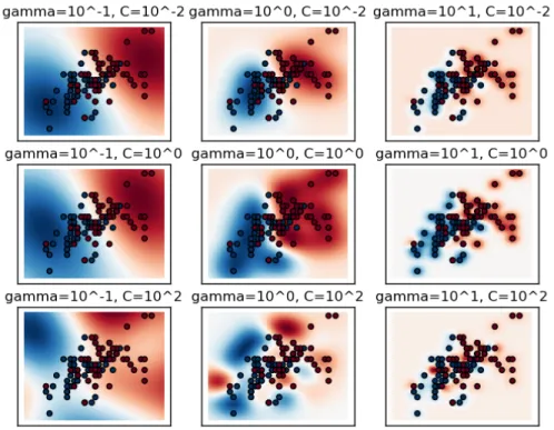
𝛾 = _2𝜎12. Figure 3-5 shows the effect of varying the parameters 𝐶 and 𝛾 using a

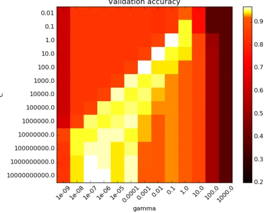
Gaussian kernel on a simple dataset. As 𝐶 increases (down the graphs), we require a decision boundary that has less miss-classifications. As 𝛾 increases, (towards the right of the graphs), the influence of each training example decreases. Figure 3-6 shows the resulting validation accuracy when we vary 𝐶 and 𝛾 through a larger range.

Hence, in the SVM model performed in chapter 5, we determine 𝜃, the weights of each feature set, 𝐶, the regularization coefficient, and 𝜎, the width of the Gaussian kernel.

Figure 3-5: Figure showing the visual effect of varying Gaussian kernel SVM param-eters, 𝐶 and 𝛾 [2]

Figure 3-6: Figure showing Validation Accuracy from varying 𝐶 and 𝛾 parameters in SVM with Gaussian kernel [2]

Chapter 4

Data Preparation

This chapter will outline the sources of data and how the data is preprocessed to generate input features. In particular, we outline the construction of some of the technical indicators and examine the various sentiment data inputs.

The S&P500 index data is obtained for the 10-year period January 1st 2006 to December 31st _{2015 from the CRSP U.S. Stock database, which contains}

end-of-day and month-end prices on primary listings for various exchanges along with basic market indices. The sentiment data from the same time period is obtained from the WRDS SEC Analytics Suite - Readability and Sentiment Analysis.

4.1

Feature Generation

In generating technical indicators to be used as input features for machine learning algorithms, we use domain knowledge from technical analysis. While the technical analysis field includes a wide range of different methods and techniques, we will focus on popular methods rather than complex or computationally expensive ones. We group and explain the different types of indicators below and detail the full set of indicators with their descriptions and formulas in Appendix A.

We use five types of technical indicators as input features:

1. Price indicators:

∙ Price indicators are based on moving averages of the daily closing price. We use both simple moving averages and exponential moving averages. Signals are also generated when the price moves outside of two standard deviations from the simple moving averages. We vary window sizes used for moving averages.

2. Momentum and reversion indicators:

∙ Momentum and reversion indicators are based on identifying trends and mean reversion patterns. Trends are found by examining differences in prices and rate of price changes across different window sizes. Mean rever-sion identification signals are generated by examining the convergence and divergence of moving averages.

3. Stochastic oscillator indicators:

∙ Stochastic oscillator indicators measure the relative level of the close price in relation to the maximum and minimum of previous close prices. Signals are also generated when comparisons indicate the market is overbought or oversold.

4. Volatility and return indicators:

∙ Volatility and return indicators evaluate the widening of the range between high and low prices, and use models to compute the estimated return over varying window sizes. Signals are generated with there are large increases or decreases in these measures.

5. Volume indicators:

∙ Volume indicators analyze positive and negative volume flows which are indicative of market reversal. Various oscillators and volume based in-dices create signals for bull or bear markets when the inin-dices cross moving averages.

Including the daily volume, the open, high and close price, we generate 183 tech-nical indicators.

Our total feature space also includes market sentiment data from the WRDS SEC Analytics Suite. This database provides sentiment measures by processing SEC filings and provide bag-of-words text analysis.

These sentiment measures provide various methods of counting the number of positive versus negative words. They also analyze the litigious and uncertain nature of the documents. A full description of the sentiment measures are provided in Appendix A. This database provides us with an additional 31 features. Hence, our total feature space is x∈ R214.

For our class labels, we define:

𝑦_𝑡𝑖 =

{︃ sign(𝑝𝑐,𝑡+1− 𝑝𝑐,𝑡) if 𝑝𝑐,𝑡+1− 𝑝𝑐,𝑡≥ 𝜖 (4.1)

0 otherwise (4.2)

Such that 𝑦_𝑡𝑖 ∈ {−1, 0, +1}, where 𝜖 is a threshold parameter determined via cross validation. Essentially, the class labels are +1 when the next day’s close price is significantly greater than today’s close price, and −1 if it is significantly less than today’s close price. If the close prices are not significantly different, then the class label is 0.

data points with 𝑁 𝑎𝑁 values in their feature space, we obtain 2399 data points. We use 80% of these data points as for training and the remaining 20% for out-of-sample testing. Hence, our training dataset xtrain ∈ R1919x214, and testing dataset

Chapter 5

Trading System Results

This chapter examines the process of parameter optimization for each of the 3 ma-chine learning algorithms applied to the feature space described in chapter 4. Each classifier’s performance on out-of-sample data is then examined in terms of both test error and cumulative returns.

5.1

Neural Network

Our 2-layer neural network is formulated as:

𝑓𝑘(𝑥, 𝑤) = 𝑔( 𝑗=𝑀 ∑︁ 𝑗=0 𝑤_𝑘𝑗2 𝑔( 𝑖=𝑑 ∑︁ 𝑖=0 𝑤_𝑗𝑖1𝑥𝑖))))

5.1.1

Parameter Optimization

There are 3 parameters we wish to optimize for our NN. First, there exists the 𝜖 parameter used as a threshold to determine class labels, defined in equation (4.1). Second, there are parameters 𝑀 , the number of nodes in the hidden layer, and 𝜆,

the regularization parameter, which determines the weight given to the cross-entropy errors and weights, (𝑤1_{, 𝑤}2_).

To find the optimal parameters, we vary 𝜖 based on the sizes of daily differences in closing price, 𝑝𝑐,𝑡− 𝑝𝑐,𝑡−1, and choose threshold values corresponding to {0th, ..., 70th}

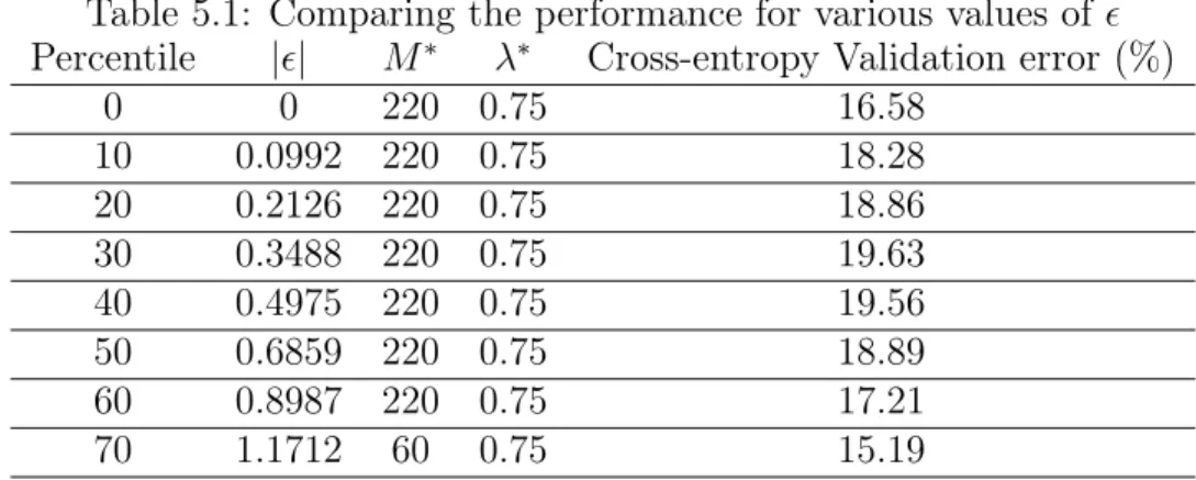
percentiles of all daily differences in the training data. Table 5.1 shows 𝑀* and 𝜆* found for each corresponding threshold when we vary 𝑀 ∈ {20, 60, ..., 220} and 𝜆 ∈ {0, 0.25, 0.5, 0.75}, where we have used 20% of our training dataset for validation.

Table 5.1: Comparing the performance for various values of 𝜖 Percentile |𝜖| 𝑀* 𝜆* Cross-entropy Validation error (%)

0 0 220 0.75 16.58 10 0.0992 220 0.75 18.28 20 0.2126 220 0.75 18.86 30 0.3488 220 0.75 19.63 40 0.4975 220 0.75 19.56 50 0.6859 220 0.75 18.89 60 0.8987 220 0.75 17.21 70 1.1712 60 0.75 15.19

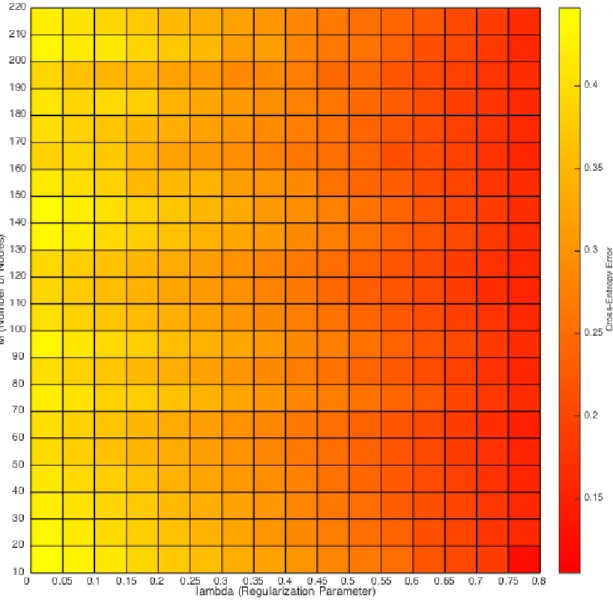
We then optimize our NN with 𝜖* = 0.7 and find that the optimal set of parameters 𝑀 = 130 and 𝜆 = 0.8 yield a cross-entropy error of 14.36%, which corresponds to an empirical accuracy of 66.67% on the total training dataset. The model selection grid search can be seen in Figure 5-1.

5.1.2

Out-of-sample Results

We test our optimized NN on the out-of-sample data, computing ˆ𝑦 = 𝑓*(xtest; w*, 𝑀*, 𝛾*)

and find a cross-entropy test error of 19.7%, corresponding to an empirical test accu-racy of 56.0%. Figure 5-2 shows the convergence of the NN on the training, validation and test data.

Figure 5-1: Figure showing cross-entropy error from varying 𝑀 and 𝛾 parameters in NN

Next, we define the trading strategy based on the predicted direction of the next day’s returns to be:

Figure 5-2: Figure showing convergence of NN on training, validation and test data

𝑟strategy,𝑡 = ˆ𝑦𝑡· 𝑟S&P500,𝑡

, where 𝑡 ∈ {1, ..., 480} are days in the test period, ˆ𝑦𝑡 ∈ {−1, 0, +1} is the

pre-dicted label at time 𝑡, 𝑟𝑡is the daily return from the position. We show the cumulative

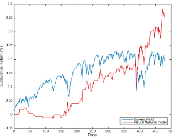
returns over the test period in figure 5-3.

For the test period, the NN model generated returns of 35.3%, compared to the market returns of 19.5%.

Figure 5-3: Figure showing cumulative return performance of optimized Neural Net-work model compared to simple buy-and-hold strategy

5.2

Random Forest

Our random forest is implemented such that for each tree,

𝑦(x) = 𝑓 ( 𝐾 ∑︁ 𝑘=1 𝑤𝑘𝜑(x,v𝑘)) =𝑓 ( 𝐾 ∑︁ 𝑘=1 𝑤𝑘I(x∈ 𝑅𝑘))

and the ensemble classifier is:

𝑦(𝑥) = 𝑀 ∑︁ 𝑚=1 1 𝑀𝑦𝑚(𝑥)

, where 𝑀 is the number of trees used in our random forest.

5.2.1

Parameter Optimization

We implement the random forest algorithm on the same dataset, keeping 𝜖 = 1.1712, which corresponds to the 70th _{percentile of daily differences.}

First, we run random forest on the dataset and find the out-of-bag classification error as we increase 𝑀 . We use out-of-bag classification error, which is a weighted misclassification rate based on all trees in the forest. That is, the predicted weighted most popular class is found for each observation that is out-of-bag for at least one tree in the forest, and the total out-of-bag classification error is empirical loss of all such predictions over all out-of-bag observations. The out-of-bag classification error is generally a better approximation to the test error than the cross-validation error [1].

Figure 5-4 shows both the out-of-bag classification error and test error when we use the full feature set x x∈ R214. We find that while the out-of-bag classification error flattens out after ≈ 150 trees, the test error’s low region corresponds to much fewer trees. This seems to suggest that using the full feature set causes the random forest to overfit to the training data.

To reduce the dimension of the feature set, we examine the importance of the features with respect to the random forest generated, as shown in figure 5-5. The names and parameters of the top 10 parameters are listed in table 5.2, with more detailed descriptions of the features in Appendix A.

Using only the top 20 parameters, we apply the random forest algorithm again to the dataset where x ∈ R20. Interestingly, we found that the reduced features don’t contain any of the market sentiment features (features 184 to 214).

Figure 5-6 shows the out-of-bag classification error for this reduced feature space as we increase 𝑀 . We select 𝑀* to be the number of trees with the lowest out-of-bag

Figure 5-4: Figure showing classification error for out-of-bag and test data as 𝑀 is increased

Table 5.2: Top 10 features in random forest ordered by decreasing feature Importance Feature Index Description

176 Negative volume index 37 Upper Bollinger band (𝑛 = 20) 139 Relative strength index (𝑛 = 20) 137 Relative strength index (𝑛 = 2) 169 Slow stochastic oscillator (𝑛 = 22)

90 Acceleration (𝑛 = 12) 151 Slow stochastic oscillator (𝑛 = 10) 143 Relative strength index (𝑛 = 24) 171 Williams indicator (𝑛 = 14)

Figure 5-5: Figure showing out-of-bag feature importance for the feature set x ∈ R214

classification error and find 𝑀* = 163.

5.2.2

Out-of-sample Results

Using 𝑀* = 163, we run random forest on the reduced feature space of the test data and find a test accuracy of 53.9%. Applying the same simple trading strategy based on the predicted direction of the next day’s returns, we find cumulative returns of 40.0% for our random forest model, compared to market returns of 19.5%. Figure 5-7 shows the cumulative returns over the test period.

Figure 5-6: Figure showing out-of-bag classification error for reduced feature set x ∈ R20

Figure 5-7: Figure showing cumulative return performance of optimized random forest model compared to simple buy-and-hold strategy

5.3

Support Vector Machines

We formulate the soft SVM optimization problem as:

max

[

]

,with a Guassian kernel:

𝐾(𝑥, 𝑦) = 𝑒𝑥𝑝(−|𝑥 − 𝑦|

2

2𝜎2 )

5.3.1

Parameter Optimization

There are two parameters we wish to optimize for our SVM model. First, there is the 𝐶 parameter that acts as a trade-off between the slack variable penalty and the margin. Second, there is the 𝜎 variable in the Guassian kernel, which determines how far the influence of each point is. We vary 𝐶 ∈ {10−2, ..., 101_{2} and 𝜎 ∈ {10}0_{, ..., 10}1_0},

and show the 10-fold cross-validation error in figure 5-8. We find that the optimal parameters occur at (𝐶*, 𝜎*) = (109_{, 10}6_{), giving us cross-validation error of 28.9%.}

5.3.2

Out-of-sample Results

Using (𝐶*, 𝜎*) = (109_{, 10}6_{), we test our SVM model on the test data and obtain a test}

accuracy of 53.1%. Applying the same simple trading strategy based on the predicted direction of the next day’s returns, we find cumulative returns of 30.3% over the test period, as shown in figure 5-9, compared to market returns of 19.5%..

Figure 5-8: Figure showing cross-validation error from varying 𝐶 and 𝜎 parameters in SVM model

5.4

Comparing the Machine Learning Models

Over the test period’s 480 days, the S&P500 index accumulated returns of 19.5%. Table 5.3 summarizes the performance of the three models compared to the S&P500.

Table 5.3: Performance comparison of the three models against a simple buy-and-hold strategy Model Return (%) Volatility (%) Prediction Accuracy % of Days above Market Buy-and-Hold 19.5 13.4 - -Neural Network 35.3 11.2 56.0 50.7 Random Forest 40.0 13.2 53.9 61.0 Support Vector Machine 31.3 9.0 53.1 43.4

Figure 5-9: Figure showing cumulative return performance of optimized SVM model compared to simple buy-and-hold strategy

We found that while the random forest model gave the highest overall return over the test period, the SVM model gave the highest Sharpe-ratio 1 _{of 3.5. However, the}

test accuracy of all three models only hovered between 50-60%.

1_{The Sharpe-ratio(SR) is a measure of risk-adjusted return, SR =} 𝑟𝑝−𝑟𝑓

𝜎𝑝 , where 𝑟𝑝= portfolio

Chapter 6

Closing Remarks

In this chapter, we conclude the paper with a discussion of the results and limitations of Chapter 5 and recommend further machine learning algorithms for creating viable trading systems. Finally, we discuss the potential areas in which further research could be done.

6.1

Conclusion

The task in this paper is to use various machine learning algorithms to predict the direction of stock price movements, using the S&P500 index as an example.

Chapter 5 explored three widely used machine learning algorithms applied to financial data to create viable trading strategies. We examined the performance of these models on the out-of-sample test sets and our empirical results showed that, despite poor prediction accuracy, the resulting trading strategies out-performed the market over this period. Our SVM model with a Guassian kernel gave us the highest Sharpe-ratio of 3.5 over this period. This is consistent with some of the results of other machine learning literature that compares different techniques [17] [24].

However, the results of the simple trading strategy based on the next day’s pre-dicted return are limited. Indeed, these trading models do not take into account market dynamics that could influence the cumulative return of the strategy. While liquidity may not be a big problem when trading a highly liquid instrument1_{, other}

factors like transaction costs, bid-ask spreads and market impact of our trades could play a big role in reducing our strategy’s returns.

It is also interesting to note the results of feature space reduction using random forest shown in figure 5-5. While our original feature space used both a number of technical analysis and market sentiment indicators, we found that the market sentiment indicators we obtained did not have very strong predictive power.

6.2

Further Work

Our analysis does not acknowledge a number of important factors that can be exam-ined in future research. First, our market sentiment indicators were drawn from a single database which compiled reports based on basic bag-of-words analysis. There is much room for improvement in this area, as natural language processing algorithms can be adapted to analyze data sources such as financial news articles, macroeconomic report or even social media, such as twitter feeds. Perhaps generating features via these mechanisms will produce better predictive features.

Moreover, while the non-linear models used in this paper successfully out-performed the market over the test period, it is unknown whether they would have as much suc-cess if market conditions changed dramatically2_{. A possible solution would be to}

create ensembles of models for subsets of time periods and use a boosting algorithm to weigh the importance of the models. Another method would be to combine the models with an evolutionary model to change the feature space through time.

1_{Such as trading the SPY, as a proxy for the S&P500 index} 2_{For example, from a high volatile to a low volatile environment}

Methods to extend the trading strategy could also be implemented. If tick-by-tick data were obtained, then high-frequency trading strategies could be examined. If mul-tiple stocks were picked, then portfolio optimization would also be a significant area of research. Those interested in applying these techniques to trading strategies may also wish to adjust the model parameters by conducting a more sensitive parameter search.

While our trading models were tested on the S&P500 index, our methods are not limited to this particular index. Further research could expand the scope of our analysis to other indices or choose a particular industry-based subset of stocks to analyze.

Appendix A

Technical Analysis and Market

Sentiment features

Table A.1: A description of all technical analysis features used

Name Description Formula

Simple Moving Average (SMA)

Simple moving average of the last 𝑛 observations of a time series 𝑃𝐶

1 𝑛 ∑︀𝑡 𝑡−𝑛𝑃 𝐶 𝑖 , 𝑛 ∈ {6, 10, ..., 50} Exponential Moving Average (EMA)

Exponential moving average of a time series 𝑃𝐶

EMA𝑡 = 𝑃 𝛼)+

EMA𝑡− 1(1 − 𝛼),

where 𝛼 = _1+𝑁2 , 𝑁 ∈ {6, 10, ..., 50}

Bollinger Bands Using the moving average, the upper and lower Bollinger bands are calculated as above and below 2 standard deviations of the closing price.

MA𝑛± 2𝜎,

𝑛 ∈ {14, 20, ..., 60}

Momentum Price change in the last 𝑛 periods 𝑃_𝑡𝐶 − 𝑃𝐶 𝑡−𝑛,

𝑛 ∈ {6, 12, ..., 60} Acceleration Difference in price change Momentum𝑡(𝑛)

-Momentum𝑡−1(𝑛),

𝑛 ∈ {6, 12, ..., 60} Rate of Change Rate of change of 𝑃𝐶

𝑡 𝑃𝑡𝐶−𝑃𝑡−𝑛𝐶 𝑃𝐶 𝑡−𝑛 · 100, 𝑛 ∈ {4, 6, ..., 60} Moving Average Convergence Divergence (MACD)

Difference between two moving averages of slow and fast periods

EMA𝑡(𝑃𝑐, 𝑠)

-EMA𝑡(𝑃𝑐, 𝑓 ),

𝑠 ∈ {18, 24, 30}, 𝑓 = 12

Name Description Formula Relative

Strength Index

Compares the days that stock prices finished up against periods that stock prices finished down.

100 − 100 1+SMA𝑡(𝑃 𝑢𝑝 𝑛 ,𝑛1) SMA𝑡(𝑃𝑛 ,𝑛1𝑑𝑛 , where 𝑃_𝑡𝑢𝑝= 𝑃𝑐 𝑡 if 𝑃𝑐 𝑡 > 𝑃𝑡−1𝑐 ,𝑃𝑡𝑑𝑛 = 𝑃𝑡𝑐 if 𝑃𝑡𝑐< 𝑃𝑡−1𝑐 , 0 otherwise, and 𝑛1 ∈ {8, 14, 20} Stochas-tic Oscilla-tor

Compares close price to a price range in a given period to establish if market is moving to higher or lower levels

𝑃𝐶 𝑡 −𝑚𝑖𝑛(𝑃𝑛𝑙𝑜𝑤) 𝑚𝑎𝑥(𝑃𝑛ℎ𝑖𝑔ℎ)−𝑚𝑖𝑛(𝑃𝑛𝑙𝑜𝑤) , where 𝑛 ∈ {10, 14, ..., 22} Williams Indica-tor

Captures moments when the market is overbought or oversold by calculating index 𝑚𝑎𝑥(𝑃𝑛ℎ𝑖𝑔ℎ)−𝑃𝑡𝑐 𝑚𝑎𝑥(𝑃𝑛ℎ𝑖𝑔ℎ)−𝑚𝑖𝑛(𝑃𝑛𝑙𝑜𝑤) , where 𝑛 = 14 Money Flow Index

Measures the strength of money flow in and out of a stock.

100 − 100 1+_{𝑁 𝑀 𝐹𝑡(𝑛)}𝑃 𝑀 𝐹𝑡(𝑛), where 𝑛 = 14, 𝑀 𝐹𝑡 = 𝑃𝑡𝑡𝑦𝑝· 𝑉 𝑂𝐿𝑡, and 𝑃 𝑀 𝐹𝑡(𝑛) = 𝑆𝑀 𝐴𝑡(𝑀 𝐹𝑡, 𝑛) when 𝑀 𝐹𝑡 > 0, 𝑁 𝑀 𝐹𝑡(𝑛) = 𝑆𝑀 𝐴𝑡(𝑀 𝐹𝑡, 𝑛) when 𝑀 𝐹𝑡< 0 Chaikin volatil-ity

Evaluates the widening of the range between high and low prices.

𝐸𝑀 𝐴(𝑃ℎ−𝑃𝑙_,𝑛) 𝐸𝑀 𝐴_𝑡−𝑛1(𝑃ℎ_−𝑃𝑙_,𝑛) − 1, where 𝑛 = 𝑛1 = 10 Nega-tive and Positive volume index

Signals of bull markets based on the volume traded and race of change of prices. 𝑁 𝑉 𝐼𝑡= 𝑁 𝑉 𝐼𝑡−1+ 𝑅𝑂𝐶𝑡(𝑛)𝑁 𝑉 𝐼𝑡−1 if 𝑉 𝑂𝐿𝑡< 𝑉 𝑂𝐿𝑡−1, and 𝑁 𝑉 𝐼𝑡−1 otherwise. 𝑃 𝑉 𝐼𝑡= 𝑃 𝑉 𝐼𝑡−1+ 𝑅𝑂𝐶𝑡(𝑛)𝑃 𝑉 𝐼𝑡−1 if 𝑉 𝑂𝐿𝑡> 𝑉 𝑂𝐿𝑡−1, and 𝑃 𝑉 𝐼𝑡−1 otherwise. Price Volume Trend

Calculates cumulative total of volume where portion of volume

added/subtracted is given by increase of decrease of close price with respect to previous period ∑︀𝑛 𝑡=1𝑉 𝑂𝐿𝑡· 𝑅𝑂𝐶𝑡(𝑛1), where 𝑛1 = 1 On Balance Volume

Evaluates impact of positive and negative volume flows

𝑂𝐵𝑉𝑡 = 𝑂𝐵𝑉𝑡−1± 𝑉 𝑂𝐿𝑡 when 𝑃𝑡𝑐 is

greater than or less than 𝑃_𝑡−1𝑐 respectively Accu- mula-tion/ Distri-bution line

Evaluates the effect of accumulative flow of money. Significant differences between the accumulation distribution line and the price produce signals.

∑︀𝑛 𝑡=1𝐶𝐿𝑉𝑡· 𝑉 𝑂𝐿𝑡, where 𝐶𝐿𝑉𝑡= 2𝑃𝑢𝑐 𝑡 −𝑃𝑡𝑙−𝑃𝑡ℎ 𝑃ℎ 𝑡−𝑃𝑡𝑙

Table A.2: A description of all market sentiment features used Name Description

Fin-Terms_Negative (Positive)

The number of Loughran-McDonald Financial-Negative(Positive) words in the document divided by the total number of words in the document that occur in the master dictionary.

Fin-Terms_Modal Weak

(Strong)_count

The number of Loughran-McDonald Financial-Modal-Weak(Strong) words in the document.

Harvar-dIV_Negative

The number and count of Harvard General Inquirer Negative words in the document.

FinTerms Count The number of Loughran-McDonald Financial Litigious, Uncertin, Modal-Weak words, both total number and percentage terms.

Bibliography

[1] Ensemble learning. http://www.mathworks.com/help/stats/ ensemble-methods.html#zmw57dd0e61659/. Accessed: 2016-04-27.

[2] Rbf parameter plots. http://scikit-learn.org/stable/auto_examples/ svm/plot_rbf_parameters.html. Accessed: 2016-04-27.

[3] Soft svm boundaries. http://slideplayer.com/slide/3362142/. Accessed: 2016-04-27.

[4] Melike Bildirici and Ozgar O. Ersin. Support vector machine garch and neu-ral network garch models in modeling conditional volatility: An application to turkish financial markets. Expert Systems with Applications, 36:7355–7362, 2009.

[5] Christopher M. Bishop. Pattern recognition and machine learning. Springer, international edition, 2013.

[6] Ganesh Bonde and Rasheed Khaled. Stock price prediction using genetic al-gorithms and evolution strategies. International Conference on Genetic and Evolutionary Methods (GEM), pages 1–6, 2012.

[7] Gerding Enrico Booth, Ash and Frank McGroarty. Automated trading with performance weighted random forests and seasonality. Expert Systems with Ap-plications, 41:3651–3661, 2014.

[8] J.H. R. Breiman, L. Friedman and C.J. Steon. Classification and Regression Tree. Wadsworth & Brooks, 1984.

[9] Leo Breiman. Random forests. Machine Learning, 45:5–32, 2001.

[10] Obradovic Zoran Chenoweth, Tim and Sauchi Stephen Lee. Embedding techni-cal analysis into neural network based trading systems. Applied Artificial Intel-ligence: An International Journal, 10:523–542, 2010.

[11] German Creamer and Yoav Freund. Automated trading with boosting and expert weighting. Quantitative Finance, 4:401–420, 2010.

[12] Erol Egrioglu, Aladag Cagda H., and Ufuk Yolcu. Fuzzy time series forecasting with a novel hybrid approach combining fuzzy c-means and neural networks. Expert Systems with Applications, 40:854–857, 2013.

[13] Eugene F. Fama. Efficient capital markets: A review of theory and empirical work. The Journal of Finance, 25:383–417, 1970.

[14] Bernd Freisleben. Stock market prediction with backpropagation networks. In-dustrial and Engineering Applications of Artificial Intelligence and Exper Sys-tems, 604:451–460, 2005.

[15] Gary Grudnitski and Larry Osburn. Forecasting s&p and gold futures prices: An application of neural networks. Journal of Futures Markets, 13:631–643, 1993.

[16] Yuan Lin Hsu, Chi-I; Hsu and Pei Lun Hsu. Financial performance prediction using constraint-based evolutionary classification tree (cect) approach. Advances in Natural Computation, 3612:812–821, 2005.

[17] Yoshiteru Huang Wei, Nakamori and Shou-Yang Wang. Forecasting stock mar-ket movement direction with support vector machine. Computers & Operations Research, 32:2513–2522, 2005.

[18] Laurent Hyafit and Ronald L. Rivest. Constructing optimal binary decision tress is np-complete. Information processing letters, 5:15–17, 1976.

[19] Laurent Hyafit and Ronald L. Rivest. C4.5: Programs for Machine Learning. San Mateo: Morgan Kaufmann, 1993.

[20] Narasimhan Jegadeesh and Sheridan Titman. Profitability of momentum strate-gies: An evaluation of alternative explanations. The Journal of Finance, 56:699– 720, 2001.

[21] Daniel Kahneman and Amos Tversky. On the reality of cognitive illusions. Psy-chological Review, 103:582–591, 1996.

[22] Boyacioglu Melek Acar Kara, Yakup and Omer Kaan Baykan. Predicting direc-tion of stock price index movement using artificial neural networks and support vector machines: the sample of the istanbul stock exchange. Expert Systems with Applications, 38:5311–5319, 2011.

[23] Kyoung-jae Kim. Financial time series forecasting using support vector machines. Neurocomputing, 55:307–319, 2003.

[24] Manish Kumar and M. Thenmozhi. Forecasting stock index movement: A com-parison of support vector machines and random forest. Int. Journal of Engineer-ing Research and Applications, 4:106–117, 2014.

[25] Zhe Liao and Jun Wang. Forecasting model of global stock index by stochastic time effective neural network. Expert Systems with Applications, 37:834–841, 2010.

[26] Andrew Lo. The adaptive markets hypothesis: Market efficiency from an evolu-tionary perspective. Journal of Portfolio Management, 30:15–29, 2004.

[27] Yu-Hon Lui and David Mole. The use of fundamental and technical analyses by foreign exchange dealers: Hong kong evidence. Journal of International Money and Finance, 17:535–545, 1998.

[28] Sam Mahfoud and Ganesh Mani. Financial forecasting using genetic algorithms. Applied Artificial Intelligence: An International Journal, 10:543–566, 2010.

[29] Lukas Mnekhoff. The use of technical analysis by fund managers: International evidence. Journal of Banking and Finance, 34:2573–2586, 2010.

[30] Kevin P. Murphy. Machine Learning A Probabilistic Perspective. MIT Press, 2012.

[31] Modhandas V.P Nair, Binoy B. and N.R. Sakthivel. A genetic algorithm opti-mized decision tree-svm based stock market trend prediction system. Interna-tional journal on computer science and engineering, 2:2981–2988, 2010.

[32] Weller Paul A Neely, Christopher J and Joshua Ulrich. The adaptive markets hypothesis: Evidence from the foreign exchange market. Journal of Financial and Quantitative Analysis, 44:467–488, 2009.

[33] Phichhaung ou and Hengshan Wang. Prediction of stock market index movement by ten data mining techniques. Modern Applied Science, 3:28–42, 2009.

[34] Shah Shail Thakkar Priyank Patel, Jigar and K. Kotecha. Predicting stock and stock price index movement using trend deterministic data preparation and ma-chine learning techniques. Expert Systems with Applications, 42:259–268, 2015. [35] Mehmet Pekkaya and Coŧkun HamzaÃğebi. An application on forecasting

exchange rate by using neural network. Congress of YAEM, 27, 2007.

[36] Ming D. Phua, P.K.H. and W. Lin. Neural network with genetically evolved algorithms for stocks prediction. Asia-Pacific Journal of Operational Research, 18:103–107, 2001.

[37] Qing-Guo; Li Jin Qin, Qin; Wang and Shuzhi Sam Ge. Linear and nonlinear trading models with gradient boosted random forests and application to singa-pore stock market. Journal of Intelligent Learning Systems and Applications, 5:1–10, 2013.

[38] J.R. Quinlan. Improved use of continuous attributes in c4.5. journal of Artifical Intelligence Research, 4:77–90, 1996.

[39] D.K Sahoo, A. Patra, Mishra S.N., and M. R. Senapati. Techniques for time series prediction. International Journal of Research Science and Management, 2, 2015.

[40] Hersh Shefrin. Beyond Greed and Fear: Understanding Behavioral Finance and the Psychology of Investing. Oxford University Press, 2 edition, 2002.

[41] Robert J. Shiller. From efficient markets theory to behavioral finance. Journal of Economic Perspectives, 17:83–104, 2003.

[42] Miller-Keith L. Sorensen, Eric H. and Chee K. Ooi. The decision tree approach to stock selection. Journal of Portfolio Management, 27:42, 2000.

[43] Miller-Keith L. Sorensen, Eric H. and Chee K. Ooi. Stock market trading rule discovery using two-layer bias decision tree. Expert Systems with Applications, 30:605–611, 2006.

[44] Mark P Taylor and Hellen Allen. The use of technical analysis in the foreign exchange market. Journal of international Money and Finance, 11:304–314, 1992.

[45] Allan Timmermann and Clive W.J Granger. Efficient market hypothesis and forecasting. International Journal of Forecasting, 20:15–27, 2004.

[46] Chang Laiwan Yang, Haiqin and Irwin King. Support vector machine regression for volatile stock market prediction. IDEAL, 2412:391–396, 2002.

[47] Shang-Wu Yu. Forecasting and arbitrage of the nikkei stock index futures: An application of backpropagation networks. Asia-Pacific Financial Markets, 6:341– 354, 1999.

[48] Yudong Zhang and Lenan Wu. Stock market prediction of s&p 500 via combi-nation of improved bco approach and bp neural network. Expert Systems with Applications, 36:8849–8854, 2009.