Analysis of acoustic communication channel characterization data in the surf zone

Analysis of Acoustic Communication Channel

Characterization Data in the Surf Zone

by

James Willard Partan

B.A., Williams College, 1994

Submitted to the Department of Electrical Engineering and Computer Science

in partial fulfillment of the requirements for the degree of

Master of Science in Electrical Engineering

at the

MASSACHUSETTS INSTITUTE OF TECHNOLOGY

and the

WOODS HOLE OCEANOGRAPHIC INSTITUTION

September 2000

@James

W. Partan 2000. All rights reserved.

The author hereby grants to MIT and WHOI permission to reproduce paper and

electronic copies of this thesis in whole or in part and to distribute them publicly.

Author ...

Department of Electrical Engineering and Computer Science,

Massachusetts Institute of Technology,

and the Joint Program in Oceanography and Oceanographic Engineering,

Massachusetts Institute of Technology/Woods Hole Oceanographic Institution

-- '7 .

I

August 4, 2000

Certified by ..

Accepted by..

...

James C. Preisig

Assistant Scientist, Woods Hole Oceanographic Institution

Thesis Supervisor

. Michael SfIFriantafyllou

Chair, MIT/WI4OI Joint

mptt,

ofiicean9gjhspjEngi

neering

A d b

cep t yU . .. . ... . . . . .. . . . ..

Arthur C. Smith

Chair, MIT Electrical Engineering Department Committee on Graduate Students

MASSACHUSET TS INSTITUTE

OF TECHNOLOGY

_BARKER

Analysis of Acoustic Communication Channel Characterization Data in

the Surf Zone

by

James Willard Partan

Submitted to the Department of Electrical Engineering and Computer Science on August 4, 2000, in partial fulfillment of the

requirements for the degree of Master of Science in Electrical Engineering

Abstract

A channel characterization experiment for the underwater acoustic communication channel was carried out at Scripps Pier in May 1999. The experiment investigated acoustic transmission in very shallow water and breaking waves. In analyzing the data, several questions arose.

The majority of the acoustic channel probe data was corrupted by crosstalk in the receiver array cable. This thesis investigates methods to correct for the effects of the crosstalk, to attempt to recover the channel probe data. In selected regions, the crosstalk could be removed quite effectively using a linear least-squares method to estimate the crosstalk coefficients. The bulk of the data could not be corrected, however, primarily due to crosstalk from a receiver channel which was not recorded, and hence could not be well estimated.

A second question addressed by this thesis is concerned with acoustic propagation in shallow water under bubble clouds. The breaking waves injected air deep into the water column. The resulting bubble clouds heavily attenuated acoustic signals, effectively causing total dropouts of the acous-tic communication channel. Due to buoyancy, the bubbles gradually rise, and the communication channel clears. The channel clearing was significantly slower than predicted by geometric ray acoustic propagation models, however. Proposed explanations included secondary, unobserved, breaking events causing additional bubble injection; delayed rising of bubbles due to turbulent currents; or failure of the geometric ray model due to suppression by bubble clouds of acoustic signals which are not along the geometric ray paths. This thesis investigated the final hypothesis, modeling the acoustic propagation in Scripps Pier environment, using the full wave equation mod-eling package OASES. It was determined that the attenuation of the propagating acoustic signal is not accurately predicted by the bubble-induced attenuation along the geometric ray path.

Thesis Supervisor: James C. Preisig

Acknowledgments

First, I would like to sincerely thank my advisor, Jim Preisig, for his patience, positive atti-tude, advice, and expertise. I would especially like to thank Mark Johnson for his extensive help on all matters and for his friendship. Thanks also to my friends and colleagues at the Woods Hole Oceanographic Institution, including Patrick Miller, Nicoletta Biassoni, Jon Woodruff, Doug Nowacek, Lee Freitag, Gene Terray, Matt Grund, Tom Hurst, Alex Shorter, and many others. Most importantly, thanks to my parents and brother for their love and support.

For financial support, thanks to the National Science Foundation for funding me on a Graduate Research Fellowship, and thanks to the WHOI Education Office for supplementing that fellowship.

Contents

1 Introduction ₅

1.1 Background .. ... .. ... ... 5

1.2 Experimental Approach . . . . 6

1.3 Data Analysis, Crosstalk Correction, and Propagation Modeling . . . . 8

2 Scripps Pier Hydrophone Cable Crosstalk: Analysis and Correction ₉ 2.1 _{Introduction and Motivation . . . . 9}

2.2 Crosstalk M odel . . . . 11

2.3 Crosstalk Correction . . . . 13

2.4 R esults . . . . 23

2.5 Alternative approaches . . . . 29

2.6 Conclusions . . . . 29

3 Acoustic Propagation Modeling in Bubble Clouds 32 3.1 Introduction and Motivation . . . . 32

3.2 Modeling Approach . . . . 33

3.3 R esults . . . . 47

3.4 Conclusions . . . . 63

Chapter 1

Introduction

1.1

Background

Very shallow water and the surf zone present a challenging channel for underwater acoustic commu-nication. Characteristics of the channel include rapidly varying multipath structure and associated fading, high levels of ambient noise, and periodic channel dropouts where signal transmission is impossible.

Most of the past work in acoustic underwater communications has been done in relatively deep water, and even the work in shallow water - roughly defined as regions where the transmission range is greater than ten times the water depth - has avoided the adverse conditions of the surf zone[1, 18].

Recently, however, there has been interest in extending underwater acoustic communication net-works into very shallow water and the surf zone, in particular for mine location and clearing operations conducted by small autonomous underwater vehicles. Underwater communication net-works will provide command and navigation data from master nodes to the vehicles, and high-rate data uplink from the vehicles to the nodes. Characterization of the channel in the surf zone would allow the communication systems to be closely matched to the environment, by determining what the best frequency bands are, what modulation methods can be supported, and what coding and protocols will be necessary. In addition, understanding the correlation of the channel parameters with environmental conditions will allow realistic expectations for the performance of the commu-nication system, given a site's particular bathymetry, wind, and sea states[14].

Over the past few years, several major scientific experiments have been conducted to study the acoustic transmission properties of the surf zone, but the experiments have concentrated on the physics of air-sea interactions and breaking waves, rather than determining engineering parameters for the underwater acoustic communication channel[20, 19]. The primary goal of these acoustic experiments has been to study the bubbles formed in breaking waves, which are the main source of both ambient noise and attenuation in the surf zone. Heavy attenuation can lead to total channel dropouts, which can last for over a minute, with attenuations of up to 26 dB/meter[6]. The past experiments have mainly examined the higher frequency bands, where most of the bubble reso-nances lie. From an acoustic communications perspective, however, characterization of the bands with less impact from bubbles, in the range from approximately 4-20 kHz, is more important. Lower frequencies are less attractive because low-frequency transducers are too bulky for use on a small vehicle, and because diffraction effects become more pronounced as the acoustic wavelength becomes non-negligible compared with inhornogeneities in the propagation environment. Higher frequencies, while offering a larger bandwidth, are attenuated more severely by the bubbles, and

are incompatible with readily-available existing acoustic communication hardware[22].

In addition to bubbles formed in breaking surf, another major problem for communication in the very shallow water channel will be the rapidly varying multipath structure[2]. The slow multipath evolution is driven by the tidal cycle, while the rapid multipath fluctuation is primarily due to scattering from the surface wave field. Fluctuation of the multipath impulse response leads directly to a finite channel coherence time, the length of which will heavily influence the design of modula-tion schemes and packet sizes. Measurements of the Doppler spreads of individual arrivals within the multipath structure, and of the angle of arrival of the different paths, could help in designing adaptive beamforming array equalizers to select the minimally-Doppler-spread direct path arrival.

1.2

Experimental Approach

In May 1999, a large channel characterization experiment was conducted at the Scripps Institution of Oceanography (SIO). Its purpose was to characterize the acoustic telemetry channel in very shallow water and the surf zone. The motivation for this work was to aid in the development of reliable communication methods for the surf zone environment.

The probe signals were chosen in order to characterize as many parameters as possible of the time-varying communication channel. In particular, the transmission loss and ambient noise, available bandwidth, the multipath structure and its time-delay spreading, and the coherence time, all needed to be measured. An ideal probe signal would be similar to a data packet, i.e. approxi-mating white noise, filling the frequency band of the transmitter, and as long as a data packet. Repeated maximal-length pseudorandom noise sequences (M-sequences) match these requirements well, particularly for phase-shift key (PSK) direct-sequence spread spectrum signals. They have an autocorrelation resembling that of white noise, and provide a high processing gain[16]. In addition, all of the parameters mentioned above can be determined from processed maximal-length sequence transmissions, using standard approaches to channel characterization[8]. The Scripps Pier experi-ment primarily transmitted M-sequences and pseudorandom sequences with similar properties.

In addition to the transmission of acoustic channel probes, simultaneous and comprehensive mea-surements of the physical environmental conditions driving the time-varying channel were made. These additional physical measurements included fairly simple measurements, such as tidal cycle, wind speed and direction, and overhead video of the site, as well as more involved spatial and temporal measurements of the underwater bubble cloud locations and bubble size distribution, the current fields advecting the bubble clouds, and array measurements of the wave and temperature fields[5].

The acoustic channel probe signals were transmitted from several different sources, covering the frequency bands from 4-20 kHz. These sources were located on both sides of the heaviest surf, so that during channel dropouts in the surf zone, the hydrophones on either side of the breaking waves would still receive some signal. The hydrophones were deployed in a large horizontal array extending approximately 300 meters across the surf zone. At the ends of the horizontal array, there were two smaller vertical arrays, each roughly spanning the vertical water column.

Each packet of probe signals was preceded by a frequency-shift key (FSK) sequence to act as a synchronization signal for data processing. The FSK synchronization signal has been well-tested, and is robust in multipath channels, whereas a phase-shift key (PSK) modulation technique, as was used for the M-sequence probes, may not be adequate for synchronization due to channel coherence limitations and ambient noise levels. In addition to the synchronization and M-sequence probes, small packets of sample communication packets were transmitted, testing various modu-lation schemes. The entire packet of signals was repeated up to several times per minute, sharing

transmission time with a sonar system which was used to map the bubble clouds.

1.3

Data Analysis, Crosstalk Correction, and Propagation

Modeling

Although the Scripps Pier experiment produced a very valuable data set overall, many of the hy-drophone channels were heavily contaminated by crosstalk. Chapter 2 of this thesis investigates methods to estimate the crosstalk coefficients between channels, and to then correct the recorded signals for the crosstalk. Correcting the acoustic probe recordings for the crosstalk would recover a critical piece of the overall environmental measurements.

With breaking waves injecting bubble clouds into the water column, the surf zone often has long channel outages. The communication system's protocol, coding, and modulation must take into account these extended outages. In order to model system performance and test new techniques, realistic models of the surf zone environment must be created. After analysis of the Scripps Pier channel characterization data, it was also determined that there was possibly a discrepancy in the time for the acoustic communication channel to clear between modeled and measured results. The time for the acoustic communication channel to clear after an outage was measured, then modeled with a geometric ray model for acoustic propagation. The discrepancy between these results led to the investigation in Chapter 3 of this thesis, in which a full wave equation propagation model was used to model acoustic propagation in the surf zone.

Chapter 2

Scripps Pier Hydrophone Cable

Crosstalk:

Analysis and Correction

2.1

Introduction and Motivation

A primary goal of the May 1999 experiment at Scripps Pier was to determine correlations be-tween environmental conditions and the time-varying characteristics of the underwater acoustic communications channel. Therefore, in addition to the three groups characterizing the surf zone communications channel, two additional teams of investigators were simultaneously measuring many environmental variables at high temporal resolutions[2 1]. The resulting data sets of acoustic channel probes and local physical conditions are very valuable, and would be extremely time-consuming and expensive to reproduce.

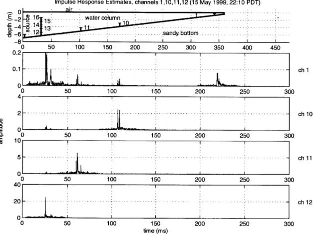
During the course of the Scripps Pier channel characterization experiment, it was noticed that signals were appearing simultaneously on widely-separated hydrophones, without the expected acoustic propagation delay, as shown in Figure 2-1. This problem was later traced to a systematic miswiring of the hydrophone cable, which capacitively coupled the channels together. The energy in these crosstalk signals was roughly 35 dB lower than the energy in the acoustically-received signals creating them. The transmission loss across the channel, however, was almost always over 40 dB, so the crosstalk signals were in general stronger than the acoustically-received signals on

Impulse Response Estimates, channels 1,10,11,12 (15 May 1999, 22:10 PDT) 0 50 100 150 200 250 300 350 400 450 0.2[ I I 0 50 100 150 200 250 3 4.2 .. - -. .- ---- - ; - -. --- - - -- -- -- -- . -- - -- -- - - - - -- - - -- -- - - . .- -0 50 100 150 200 250 3( 50 100 150 200 250 3 40 0 L 0 50 100 150 200 250 30 time (ms) ch 1 0 ch 10 ch 11 0 ch 12 0

Figure 2-1: The top plot shows the Scripps Pier geometry, with the hydrophone locations labelled by hydrophone number, and the horizontal axis in meters. The lower four plots show the impulse response estimates on hydrophones 1, 10, 11, and 12, when transmitting from deep-water source 4. Note the different amplitude scales.

U)

0

0

channels where the hydrophone was distant from the source. The crosstalk problem was most severe for hydrophones distant from the transmitting source, since the recorded signal was domi-nated by the crosstalk.

With the fairly strong crosstalk which existed, signals which were longer than the propagation delay of the channel were mixed together. Some of the data could be processed to yield estimates of the channel impulse responses. None of the data containing crosstalk, however, is useful for testing communication algorithms or performance. The acoustic propagation delay for the entire channel, covering about 300 m, was about 200 ms. Between neighboring hydrophones, however, a typical propagation delay was about 50 ms, corresponding to roughly 70 m. Signals longer than these propagation delays, and also continuously repeated signals, would have been mixed together by the crosstalk, as an inshore hydrophone would simultaneously receive an acoustic signal and a crosstalk signal from a later part of the transmitted sequence, coupled in from a deep-water hydrophone.

2.2

Crosstalk Model

The crosstalk was caused by a wiring mistake in the hydrophone cable. A shielded pair of cables carried the signal from each hydrophone back to the hydrophone cable breakout box, the pream-plifier, and the recorder. Rather than being connected together and tied to a salt water ground, the individual shields were connected to the negative input on each channel. The shields lay next to one another in the hydrophone cable for as much as 300 m, and the capacitive coupling between the shields, directly connected to the negative input of each channel, led to the crosstalk.

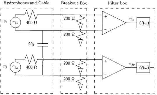
An AC circuit model of a pair of channels, including hydrophones, breakout box, and preamplifier, is shown in Figure 2-2. The hydrophones, which were used in current mode, are modeled as voltage sources in series with a resistor; equivalently, they could be modeled as current sources in parallel with a resistor. The capacitive coupling between channels i and

j

The circuit can be analyzed through superposition. When there is no voltage on hydrophone i, the entire signal at the output of channel

j,

Hydrophones and Cable Vj e 400 Q Vi _{V-L 400 Q} L - - - - - - - - 1--- -1-- -4-Breakout Box 1 200 Q 200 Q 200 200 Q L -H-I Filter box + vio G(w) -+ SG(w) -_-I _ _ _ _

Figure 2-2: An AC circuit model of the hydrophones and hydrophone cable, breakout box, and filter box. The shield-to-shield capacitance Cij couples channels i and

j.

on channel

j.

Vio = 400 Q - I = 1vj.

When there is no voltage on hydrophone

j,

j

1 _200Q

(Vi) 2 Zc + 200 _{Q600 Q 4/}

where the impedance of the capacitor is Zcj = 1/iwCij, and 11 indicates parallel connection of components.

directly, is

1 1

~200

Voj = 2 V + 8 Zcj + 200 Q||600 Q Vi = V + JVi,

i j i#j

where aij is the crosstalk coupling coefficient between channels i and

j,

Finally, the assumption that the current flowing in the coupling capacitor can be neglected com-pared with the current flowing directly in the resistor networks needs to be checked. The mea-sured crosstalk coefficients have magnitudes of roughly -35 dB to -40 dB, at a carrier frequency of 11.5 kHz. Using the model above, this gives a coupling capacitance value of around 3 nF, which is consistent with typical conductor-to-conductor capacitances over several hundred meters of cable.1 The model gives plausible predictions for the coupling capacitance, and at these capacitances, the current through the coupling capacitor is less than 5% of the total current flowing in the resistor network, so the approximations made above are valid.

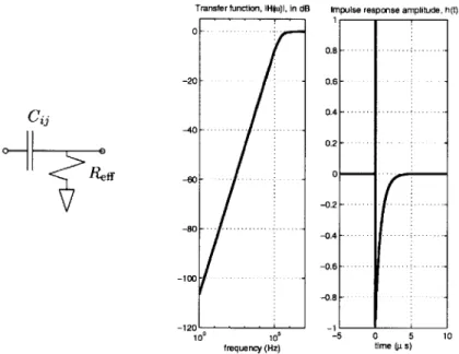
The circuit model above can be further reduced to an effective high-pass filter coupling the channels, shown in Figure 2-3a. The effective resistance is Rdf = 150 Q, and the capacitance is the coupling capacitance, Cij, estimated to be 1 nF to 10 nF. The characteristic time constant for this circuit is then on the order of 1 is or less. The transfer function of this system is

iw ReffC--2

H (w) = wReff C = iwReffCij(1 - Reff Cij + 0(w2

RffCij)),

1 + jWReffCj

and its magnitude and phase are plotted in Figure 2-3b, for Cij = 10 nF, which has the slowest rise time for our range of interest in Cij. Over the frequency band of interest, 9-14 kHz, the phase is nearly constant, and the magnitude is a linear function of frequency.

2.3

Crosstalk Correction

With a model of the crosstalk, the next step is to estimate the crosstalk coefficients, and correct the recorded signals.

1

Datasonics measured the coupling capacitances in the cable after the experiment, and came up with typical values of 30 nF to 90 nF (see Table 2-2). These values would give crosstalk coefficients on the order of -20 dB to -12 dB in this model, which are much stronger than the observed crosstalk. The resistor network in the breakout box is well-known, and the error causing the crosstalk is well-known, so it is likely that the actual coupling capacitances were somewhat smaller, in the range of 1 nF to 10 nF.

Transfer function, Hto)I, in dB Impulse response amplitude, h(t) 0 - --.... 0.8 -- - - .... -20 - 0.6 -Cij

~~0.4

Figure 2-3: (a) The effective high-pass filter, (b) its transfer function, and (c) its impulse response.

The primary channel characterization signals which were transmitted were length-511 binary phase-shift key (BPSK) maximal-length pseudo-random sequences (M-sequences). When an M-sequence is cross-correlated against a repeated train of the same M-sequence, the result approximates a train of impulses, with low sidelobes. In channel characterization experiments, a train M-sequences is transmitted through the acoustic communication channel. The recorded signal is the convolution of the M-sequence train with the channel impulse response. Cross-correlating the recorded signal with the transmitted M-sequence yields a series of channel impulse response estimates, which track the evolution of the time-variant channel[16].

Due to the crosstalk mixing in the Scripps Pier experiment, the cross-correlation of the baseband data for a given channel will not directly yield an impulse response estimate for that channel, but rather a superposition of the impulse response estimates for all the channels. Once crosstalk was determined to be a significant problem, additional characterization probes were added, namely short length-88 Turyn codes. Cross-correlation of isolated length-88 Thryn codes also yields an impulse response estimate, with a peak-to-maximum-sidelobe amplitude ratio of 88/5, or about 25 dB[12]. The cross-correlation of length-511 M-sequences has a peak-to-sidelobe amplitude ratio of 511, or 54 dB, so almost 30 dB of peak-to-sidelobe power was lost by switching to length-88 Turyn codes[16]. Due to their short length, however, 22 ms at 4000 symbols/sec, these Turyn codes can be range-gated at each hydrophone, and by doing that, individual, uncontaminated estimates

of the crosstalk coefficients can be made for each channel.

If the crosstalk coefficients are constant over time, then the bulk of the data, including the long sections of repeated M-sequences, can be pre-corrected for crosstalk, then processed as usual for channel characterization. This is especially important because of the simultaneous environmental measurements made by the teams from Scripps Institution of Oceanography (SIO) and Institute of Ocean Sciences (IOS). Combining these measurements with the extensive acoustic channel probes creates a potentially very valuable data set for correlating the environmental conditions to the acoustic communication channel parameters which they drive.

Coefficient Estimation

To analyze the crosstalk coefficient estimation, let sj [k] be the baseband signal received acoustically at hydrophone

j

j

With crosstalk, the signal recorded from hydrophone

j

or,

rj[k] = sj [k] +E a si [k] + n[k].

The a, are unknown dimensionless crosstalk coefficients to be estimated for coupling channels i to channel

j.

i.e. a single coefficient per channel.

In the regions where the crosstalk coefficients are to be estimated through range-gating, there is essentially no real signal in sj[k]; it can therefore be combined into the noise term, n[k]. Since the acoustically-received signals si[k] were not preserved directly, they can be approximated as the baseband recorded signals ri[k], which is a reasonable approximation. The model then reduces to

rj[k] = E a ri[k] +n[k]. (2.1)

i:/i

This model can then be written as Ra + n = rj, where R is a matrix formed of the baseband recorded signals ri, taken as column vectors, and rj and n are the recorded signal and effective additive noise, respectively, again taken as column vectors.Underlining or bold face indicates vector quantities. Equivalently, the model could be written in terms of the impulse response estimates of

the channel, hi[n], rather than the baseband recorded signals, ri[n], since a linear transformation relates the two, namely cross-correlation with the transmitted signal.

In the model Ra+ n = rj, the noise vector

n

a

&r = (RH R)--R Hrj = a + (RH R) RH

Variance of coefficients, baseband signals versus impulse response

esti-mates

The coefficient estimates can be made either with the baseband signals, or with the impulse response estimates resulting from matched-filtering the baseband signals with the baseband trans-mitted waveform. The method producing more robust estimates will be preferable.

From the previous section, the model for the crosstalk is

Ra + n = r3. (2.2)

In this expression, R is a matrix, and its columns are the recorded signals from the channels which dominate the crosstalk (offshore channels 10-15). The recorded signal on an inshore hydrophone (channels 1-6) is represented by the column vector rj. In the crosstalk model, during the time before the acoustic signal has propagated to the inshore hydrophones, the only contributions to the received signal rj are noise and crosstalk. The column vector n is a zero-mean white noise vector. The crosstalk is expressed as the product between R and a. In the case of a single-tap crosstalk model, where a length-1 filter, or constant gain term, represents the crosstalk transfer function, a is a column vector of crosstalk coefficients between all of the offshore channels (channels 10-15) and the inshore channel to be corrected (only one of channels 1-6). For multiple-tap crosstalk models, a would be a matrix with as many columns as there were taps in the model. For simplicity, the remainder of this section will be restricted to single-tap models.

The linear least-squares estimate of a is

as shown in the previous section. The matrix R can be written as R = R, + N, where R, is a

matrix of the received signals due to deterministic propagation through the channel at a particular instant, and N is a noise matrix containing the received noise column vectors for each channel. The noise at any pair of hydrophones is uncorrelated, and furthermore it is modeled as zero-mean white noise. Because of these assumptions, N and n are uncorrelated. The expectation value of &, is

E[,= + E [(RH R)-1RHn

= a+E[(RH _{R)-'RH] E[n] =a,}

since N (as an additive component of R) and n are uncorrelated, and n is zero-mean. Therefore,

&, is an unbiased estimator of a.

Now consider filtering the baseband signal with a matched filter. For the transmitted signal s[k], with energy E., the matched filter is s,[-k]/E,. Defining the matched-filtered data as mj[k] = rj[k] * s.[-k]/E, and applying the matched filter to Equation 2.1 yields

mj [k] =

Z

i:/j

In this expression, the noise vector, n', is still approximately a white noise, zero-mean vector, since the matched filter consists of a pseudorandom sequence and provides little shaping. This can be written in matrix form as

Ala + n' = mn,

where M is a matrix of the column vectors mi. This form is directly analogous to Equation 2.2. Following the derivation of Equation 2.3, the linear least-squares estimate of a using the matched-filter data, &m, is

M= a+(MHM)-IMHn.

As with the estimator in the unfiltered baseband case, &m is an unbiased estimator of a.

Since estimators of the crosstalk coefficients in both the unfiltered and matched-filtered cases are unbiased estimators, the variance of the estimators will determine which estimator has a lower expected error; the one with the lower variance will have the lower expected estimation error.

Returning to the unfiltered baseband signal case, the covariance of the estimator is

COV(&r) = E

[,4H]

From above, E[dr] = a. The remaining term in the covariance is

E &H]d = aaH + (H g) H H

~H

g-E 11r-'J + E [(RHR-lR nnHR(RHR)l].

The crossterms vanish because they have expected value zero, due to N and n being uncorrelated. The expected value in this expression can be evaluated with an iterated expectation:

E [(RH )-lRHnn HR(RHR)-] = ER [ En|R [(RH R)-RHnn H R(RH R)-| R]] = 02E [(R H R)-RHR(RH R-]

= 02 _{E [(RHR)-}1_]

Therefore the covariance of the estimator is

Cov(&,) = o2

E [(R HR)-1].

To evaluate the expectation value in the estimator's covariance, several approximations are neces-sary. Expanding the term RHR yields

RHR= R + R HN + NHRo + NHN.

If the levels in the noise matrix N are small compared with the signal levels in R., or if the signals in the columns of R. are fairly variable, then the crossterms will be small, and can be neglected. Furthermore, if the signals in the columns of R. have little overlap, then (R'RO)ij Ej6j, where Ei is the energy in signal ri. Finally, if NHN within the expected value can be replaced with E[NH N] = 0.2I, then

Cov( ,) 2

E [(RHR)-1

Cov( ,) ~ 2E [(I+ (RH RO-1 NHN)1 (RH R)-1

2 Cov(d,)j ~ , + o 2 6ij

In the case where the matched-filtered impulse response estimates are used instead of the baseband signals, the derivation is identical, except the noise variance is different. The filtered noise vector n' is formed from the white noise sequence n[k], filtered with the matched filter, s,[-k]/E,. The matched filter is a Turyn code of length K = 88, and each sample has amplitude ±A. Since n[k] is a sequence of independent, identically-distributed samples with variance o,2, the variance of n' is

2 KA 2

,2

Var(n') = a2

The covariance of the crosstalk coefficient estimator, in the case of matched-filtered signals, is then

J2

Cov(&m)ij ~ o 2 6 i < Cov(a,)ij.

The energy E, in the Turyn code is greater than unity in this normalization, so the coefficient es-timates from the matched-filtered signals have lower variances than the eses-timates from the signals which are basebanded only. Since both estimators are unbiased estimators of the crosstalk coeffi-cients a, the estimator using matched-filtered signals will have a lower expected estimation error. This is the principal advantage of using the matched-filtered signals instead of the baseband signals. A secondary advantage of compressing the signal energy into impulse response estimates is that the impulse response estimates are easier to range-gate than the unfiltered baseband signals are. Finally, since the expected value of both estimators is the same, the crosstalk coefficient estimates from the matched-filtered impulse responses can be used to correct the unfiltered, baseband signals.

If the coefficients are stable in time, low-variance coefficient estimates obtained from the matched-filtered data using Turyn codes can be applied to other signals, including data from continuous M-sequences, where simple crosstalk coefficient estimates are impossible due to the inability to range-gate the signals.

Number of Taps

In order to correct the sampled data for crosstalk, a discrete-time model of the continuous-time crosstalk coupling must be made. The simplest approach is to model the coupling with finite impulse response (FIR) discrete-time transfer functions between the various channels. The convo-lutions resulting from FIR filtering can be immediately formulated as a linear least squares problem to estimate the tap values.

The continuous-time model derived above is explicitly frequency-dependent, since the coupling mechanism is a high-pass filter. Ideally, the discrete-time filter will be frequency-dependent as well, to capture the coupling most accurately. The simplest frequency-dependent FIR filter has two taps; a single-tap filter is just a constant gain. The energy residual from linear least-squares correction with two taps (parameters) will by definition be as small or smaller than with a single tap, for a given section of data.

With data from tape 1352210, when linear least-squares corrections were made by estimating the tap values for each impulse response estimate separately, the correction with two taps was some-what better than with a single tap. With a single tap, the mean energy residual in the crosstalk region (relative to the crosstalk energy before correction) was -9.5 dB versus -12.0 dB for two taps. Typical values for the tap coefficients are shown in Table 2-1.

The coefficients for the second tap in the two-tap filters are not stable in time, however. Some insight into this problem can be gained by considering sampling the impulse response of the continuous-time filter, plotted in Figure 2-3c. The impulse response has almost completely re-turned to zero after roughly 5 ps. The sampling rate of the system was only 48 kHz, however, corresponding to a sampling period of 20.8 ps. Since the impulse response of the effective high-pass filter is short compared with the sampling period of the data, the estimate of the second tap of a two-tap filter may be dominated by noise.

Considering the continuous time transfer function also indicates that the second tap may be heavily influenced by noise. Letting

w

we,

H (c) ~ (iW ReijCij + w Rff Cij) + D (iReff Ci + 2wc Reff C ) = A + &'B.

With typical values for Ref and Cij, A is approximately -30 dB, and B is approximately -125 dB. Any small amount of noise in the data will make B, corresponding to the second tap in a two-tap filter, extremely difficult to estimate reliably.

Single Coefficient Estimates versus Continuous Estimates

Although the energy residuals for the crosstalk correction using a two-tap filter mentioned in the previous section were slightly smaller than the residuals when using a single tap, these results were for cases where it was possible to re-estimate the tap coefficients at each impulse response. The short, isolated Turyn codes allow the crosstalk from individual channels to be identified, due to acoustic propagation delays. Continuous maximal-length sequences, however, formed the majority of the channel probe transmissions, and cannot be range-gated to estimate crosstalk coefficients in a straightforward manner.

To correct the crosstalk on the maximal-length sequences, it is therefore difficult to estimate the crosstalk coefficients for each impulse response. Instead, the crosstalk coefficients must be estimated from a section of data which can be range-gated, such as a section of Turyn code trans-missions, then those coefficients must be applied to the rest of the data, without further coefficient updates.

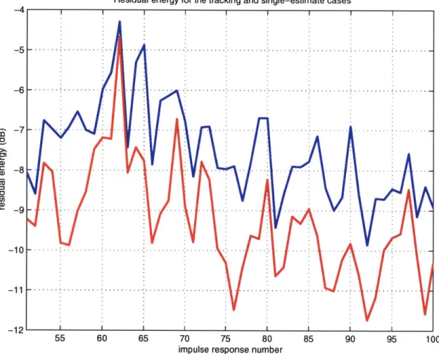
In correcting the data from tape 1352210, when the tap values were estimated from the first 49 impulse response estimates, and applied in the crosstalk correction of all later impulse response estimates, the two-tap correction was still better, but not as markedly so as in the single-tap case. With a single tap, the mean energy residual using a single initial coefficient estimate was -8.8 dB, and -9.3 dB for two-tap correction. Furthermore, these initial coefficient estimates were applied to data which was separated by at most two hours. If the tap values drift over timescales larger than an hour, the single-estimate case will end up becoming significantly worse than the tracking case, where a new estimate of the tap coefficients is made for every impulse response estimate. For timescales of up to an hour or two, however, the case with a single initial estimate did not become increasingly worse with time, when compared with the tracking case; rather, it remained at a level several dB worse than the tracking case. Figure 2-4 shows a typical sequence for the energy residuals for both the single-estimate and tracking cases.

Even though no significant long-term drift in the tap coefficients was observed, the linear least-squares estimates of their values do fluctuate significantly over short timescales, such as seconds or minutes. Because the coefficients in the second tap case are much less stable over time than the single-tap crosstalk coefficients, a single-tap, frequency-independent crosstalk correction method would be more reliable for correcting most of the data.

-4 -5 -6 -7 -8 -9 -10 -11 -12

Residual energy for the tracking and single-estimate cases

55 60 65 70 75 80 85 90 95

impulse response number

100

Figure 2-4: Plotted in blue is the residual energy after crosstalk correction using an initial estimate of the crosstalk coefficients (from the first 49 impulse responses), applied to all later data. Plotted in red is the residual energy after correction when the crosstalk coefficients were estimated for every impulse response. Both curves show the residuals for impulse responses 50-100. The residuals for the case with an initial estimate are typically 3-4 dB worse than those for the tracking estimates, even up to two hours after the initial estimates were made.

V a) C a) U) 0) - -. - - -- - - -. ---- --- - . .... . . . ... . .. . .. . .. . ... . .. .-- --- -- -- -- - -- . ..-- -- ---- --- .- ..- ---- .- -- .--- ...- ...--.. ... -. ... ... -. ... --. . --.. - -. .... .. ..-. .. . . .-.. . . . --.- . .- .- . .. ..- .. . .. .. . . .. . . . . . . . --. . .--- - - .... . . .-. .. . ... .. ... -. . . . .. . . . .---. -. -- -. . . . . .. .. .-.-. ..

The variability in the tap estimates is primarily due to fluctuations in phase, rather than magni-tude. As shown in Table 2-1, in both the one-tap and two-tap cases, the phases of the coefficients have a large standard deviation relative to their mean values, whereas the magnitudes have a small standard deviation relative to their mean values. The standard deviations in both phase and magni-tude are significantly larger for channels 13-15 compared with 10-11. Channel 12 in most cases has a larger standard deviation than channels 10-11, but not always as large as channels 13-15, which is surprising, since it is in the same vertical array and should have similar problems due to channel 16.

Table 2-1: Tap Coefficients

Channel 10 11 1 12 13 14 15 One-tap coefficients Magnitude mean 0.0174 0.0102 0.0112 0.0055 0.0136 0.0063 Magnitude st. dev. 0.0005 0.0003 0.0012 0.0008 0.0011 0.0014 Angle mean -0.3164 -0.1164 -0.8809 -0.2180 -0.9107 0.1138 Angle st. dev. 0.0334 0.0318 0.1151 0.1476 0.0786 0.2258 Two-tap coefficients

Magnitude mean (tap 1) 0.0169 0.0097 0.0111 0.0056 0.0125 0.0072 Magnitude mean (tap 2) 0.0016 0.0010 0.0022 0.0008 0.0034 0.0036 Magnitude st. dev. (tap 1) 0.0006 0.0003 0.0012 0.0008 0.0010 0.0014 Magnitude st. dev. (tap 2) 0.0006 0.0002 0.0006 0.0004 0.0016 0.0009 Angle mean (tap 1) -0.2794 -0.1007 -0.9595 -0.1375 -0.9468 0.1522 Angle mean (tap 2) -1.1586 -0.3605 -0.4354 0.2283 -0.3394 -0.5333

2.4

Results

Transmissions from outer source

For the data which was transmitted from deep-water source 4, the most important hydrophone channels are the hydrophones relatively close to shore, namely channels 1-10. These are the hy-drophones which are surrounded at times by bubble clouds, and determining their availability for communication data links was a major goal of the experiment. These are also the channels, how-ever, where crosstalk was most significant when transmitting from the outer sources, because the acoustically-received energy was in general less than the energy received from crosstalk.

In this transmission geometry, the vertical hydrophone array, channels 12-16, is very close to the source, and crosstalk is negligible, so the recorded signal on these channels can be taken to be the acoustically-received signal. Further inshore, channels 10 and 11 have crosstalk contributions from channels 12-16, but very little crosstalk contribution from the inner hydrophones, channels 1-9. The crosstalk on these innermost phones is significant, often stronger than the acoustically-received sig-nal, and is dominated by contributions from channels 12-16, 11, and 10, with only a small amount of channel-to-channel crosstalk amongst the innermost hydrophones.

With this crosstalk structure, an iterative crosstalk correction procedure can be developed. Chan-nels 12-15 are left uncorrected. (Channel 16 was not recorded, but its hydrophone remained powered during the experiment. This problem will be discussed further below.) For a given in-shore channel, the crosstalk coefficients coupling that channel to channels 12-15 are calculated in a small range-gated region of the impulse response estimate. The entire impulse response estimates for 12-15, weighted by the coefficient estimates, are then subtracted from the impulse response estimate for the inshore channel.

Next, the impulse response estimate for channel 11 is corrected for channels 12-15 in the same manner: the crosstalk coefficients between 11 and 12-15 are estimated in a range-gated region, and the entire impulse response estimates for 12-15, each weighted by a constant, are subtracted from channel 11. A crosstalk coefficient is estimated between channel 11 and the inshore channel, and the inshore channel is corrected for crosstalk from 11. This is repeated for channel 10, this time correcting channel 10 for channel 11, as well as 12-15, before correcting the inshore channel for crosstalk from 10.

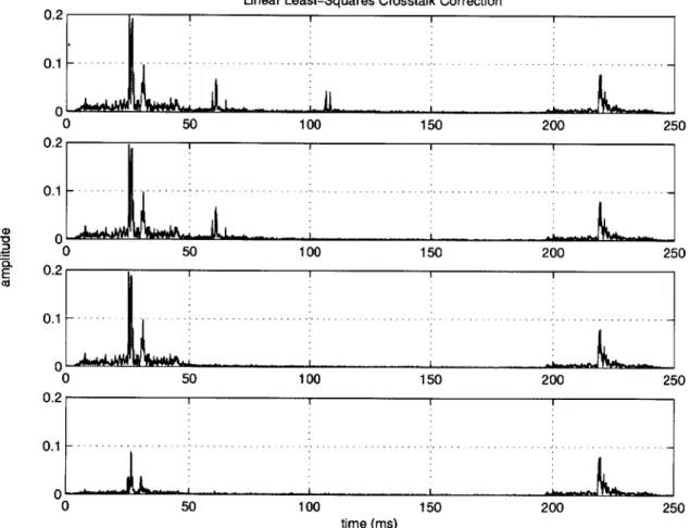
At this point, the inshore hydrophone channel has been corrected for crosstalk from all the outer hydrophones which were recorded. This removes the vast majority of the crosstalk energy con-tributed to the inshore channel, due to the high acoustically-received signal levels on the outer channels. This process is shown in Figure 2-5.

Residual energy

As shown for a single set of impulse responses in Figure 2-5, crosstalk correction using single-parameter linear least squares fitting works fairly well. The energy due to crosstalk from channels 10 and 11 can be largely removed from inshore hydrophone channels, and most of the energy due

Linear Least-Squares Crosstalk Correction 0.2 O.1 ---- - -4 -w A L- - --o

i

Figure 2-5: Frequency-independent crosstalk correction of inshore channel 1. The uppermost plot shows the uncorrected, channel 1 signal as it was recorded. Moving down, the next plots correct for crosstalk from channel 10, then channel It, then channels 12-15. The large residual remaining in the lowest plot is due to the contributions of channel 16, which was not recorded.

to crosstalk from the outer vertical array (hydrophones 12-16) can be removed as well. There is a relatively large energy residual from channel 16, however, which was not recorded, and therefore cannot be properly removed.

Figure 2-6 shows the residual energy level as a function of time after crosstalk correction on chan-nel 1. The acoustically-received energy on chanchan-nel 1 is also plotted as a baseline for comparison. The residual energy from channel 10 crosstalk is small, almost always below the acoustically-received energy for channel 1, even when there is heavy acoustic attenuation. The residual energy from channel 11 crosstalk is quite similar to that from channel 10, although it is not as consistently below the acoustically-received energy levels for channel 1. Residuals from the outer vertical array, channels 12-16, are significantly larger, almost always larger than the acoustically-received energy on channel 1. This is again because channel 16 was not recorded, and so there is always a compo-nent of the crosstalk from the outer vertical array which cannot be cancelled with this technique.

Time variability of crosstalk coefficients

The energy residuals from the previous section were obtained by estimating the crosstalk coefficient for every impulse response estimate. In order to correct sections of data where transmission was continuous, and range-gating is not possible, the crosstalk coefficients must be stable enough to allow correction without continually tracking the coefficient estimates.

In Figure 2-7, the energy residuals are plotted as a function of time, both when estimating the coefficients separately at every impulse response estimate, and when applying an initial estimate to all later times. Crosstalk coefficient variability was examined on short timescales only, up to timescales of hours, but not days.

For channels 10 and 11, there is no significant difference in correction performance between track-ing the coefficients, and ustrack-ing an initial estimate for subsequent data.

For channels 12-15, the energy residual is significantly larger when the crosstalk coefficients are not being continuously tracked. This is again due to channel 16 not being recorded, yet contributing heavily to the crosstalk.

Energy in Residuals after Crosstalk correction 0 -10 - - - ---.-.-.-.-.-.-.-.-.- -.-. 2000 2500 S - 15 -. --. - . .- - -. . . .-. -. -.. .. ... Cs E -20 -30 -35 -. -.. -... -40 0 500 1000 1500 2000 2500 0 -10 - 0-10 ₁ -15 -30 -35 -. . . .--..--.---40 0 500 1000 150 2000 2500 -5 0 - _-- -- --10 -.. --- --.-.- ---. -15 - - - ---2 0 ---. -- -. - - --.-..- . . .. .. - ...--30 -. -.-..-- -.--35 -- -. . . .. . ..-.. - --40 0 500 1000 1500 2000 2500

impulse response number

Figure 2-6: In each plot, the red curve, repeated identically in all three plots, shows the acoustically-received energy in channel 1, for comparison. The green curves shows the crosstalk energy in channel 1 from channels 10, 11, and 12, for the top, middle and bottom plots, respectively. The blue curves show the residual crosstalk energy in channel 1, after crosstalk correction, due to crosstalk from channels 10, 11, and 12, for the top, middle, and bottom plots, respectively.

time variation of crosstalk coefficients 9 -36 - I - - - -- - - -- - -- - - --- --- - --- low- -- - -k L A " - --38 -40 -44' 0 500 1000 1500 2000 25 0 500 1000 1500

impulse response number

00

2500 2000

Figure 2-7: The upper and lower plots show the time variability of the magnitude and phase, respectively, of the single-tap coefficients for channels 10, 11, and 12. Channel 10 is plotted in blue, channel 11 in red, and channel 12 in green. Channel 12 has a significantly larger variance in both magnitude and phase, due to the contribution from the uncorrected channel 16.

CA) a) a) a) as 1.5 1 0.5 0 -0.5

-

, , .i--

-

- - -

--

-- - - -

-2.5

Alternative approaches

The fundamental problem with the crosstalk correction is that channel 16 was not recorded, and hence it is very difficult to correct for its effects. In theory, it might be possible to estimate chan-nel 16 from chanchan-nels 12-15, since the hydrophones for those chanchan-nels were in a five-element vertical array.

Using array processing to beamform the signals on channels 12-15, and then estimate the signal on channel 16, is not likely to work well, however. The acoustic wavelength in a band around 11.5 kHz is about 13 cm, but the vertical array spacing was 1 m. The unambiguous range in angle before aliasing is therefore about ±60, but it is quite possible for high-angle reflections from the surface or bottom to arrive at the array.

Additional attempts to estimate channel 16 included an ad-hoc method to estimate the delay and phase of channel 16 with respect to channel 15. Using a delayed and phase-shifted version of channel 15 to approximate channel 16 was not very successful, however, again most likely due to the relatively large separation of the sensors, reducing their correlation.

Further reading was done in noise cancellation and system identification techniques, without many promising leads[23, 7]. The signal on channel 16 is qualitatively similar to those on channels 12-15, but the spatial separation is relatively large, and not precisely known, reducing the likelihood of making a good estimate of channel 16 based upon the received signals on channels 12-15. Without a good estimate of channel 16, crosstalk correction cannot be performed effectively on signals which are not range-gated.

2.6

Conclusions

The coupling between the channels can be well modeled as a high-pass filter, leading to crosstalk. This effective high-pass filter, however, has a roll-off frequency which is much larger than the sam-pling frequency of the system. Because of this, estimates of the tap coefficients of any discrete-time frequency-dependent filter which approximates the high-pass filter will not be robust in even small amounts of noise. Practical crosstalk models for this system are therefore limited to single-tap, or frequency-independent, models.

signals, has several advantages, most significantly that the variance of the estimates is lower. With single-parameter linear least-squares estimates applied to impulse response estimates, the crosstalk energy can be greatly reduced for some channels, in particular the mid-water hydrophones 10 and 11, when transmitting from deep-water source 4. For the deep-water vertical array, however, comprised of hydrophones 12-16, the residual crosstalk energy is significantly higher, since hy-drophone 16 was powered but was not recorded, and cannot be corrected for using this technique. Furthermore, the energy residuals for channels 12-16 are significantly increased when the coeffi-cients are not continuously tracked. This means that for signals which cannot be range-gated, for instance repeated maximal-length pseudo-random sequences, the crosstalk from the outer vertical array cannot be easily removed. In addition, channel 16 cannot be well-estimated from chan-nels 12-15, either through array processing or other techniques, and so the large and time-varying energy residuals due to channel 16 cannot be eliminated.

The large residuals from channel 16 are only a problem when transmitting from the deep-water sources, however: for sources which were more distant from hydrophone 16, the crosstalk is not dominated by contributions from the deep-water vertical array. There is little high-quality data from the in-shore source, however, and signals from the mid-water source are difficult to range-gate for coefficient estimation. Another possibility is to use signals from the IOS sonar, which was near the in-shore source and transmitted throughout the experiment. The majority of the codes used by the IOS sonar cannot produce impulse response estimates, however, and even for the few true pseudo-random codes which were transmitted, the processing gain is relatively low, even compared with a length-88 Turyn code.

Table 2-2: Measured Channel-to-Channel Shield Capacitance, nF (Datasonics) Channel 1 2 3 4 5 6 7 8 9 10 11 12 13]J 14 15 16 0.182 0.165 0.197 60.90 69.60 91.90 61.20 85.60 59.60 56.00 35.60 0.197 0.195 0.197 67.60 69.20 51.20 91.20 48.10 67.00 42.90 34.60 0.198 0.198 0.192 0.185 59.70 57.80 66.90 50.80 82.00 51.50 32.20 0.168 0.166 0.184 0.197 59.70 58.30 91.40 58.00 61.20 45.00 45.40 38.00 0.183 0.171 52.00 57.80 58.30 54.50 83.40 55.00 64.80 32.80 33.00 0.185 0.192 0.17 66.90 91.40 54.50 51.30 76.00 44.80 37.30 0.19 0.181 0.174 49.00 50.80 58.00 83.40 51.30 49.00 48.00 33.20 52.00 0.195 0.193 0.186 82.00 61.20 55.00 76.00 49.00 47.60 32.30 44.20 49.10 0.20 44.30 51.50 45.00 64.80 44.90 48.00 47.60 28.10 46.00 43.20 37.00 36.00 32.20 35.40 32.80 37.30 33.20 32.20 28.10 1 2 3 4 5 6 7 8 9 10 11 12 13 14 15 16 0.168 0.169 0.193 57.50 99.50 68.20 67.70 72.00 57.20 48.10 41.80 36.30 55.30 56.00 36.00 0.160 0.187 0.196 52.30 81.20 58.90 60.60 63.30 51.60 43.50 45.70 34.90 55.00 36.10 34.80 36.66 42.30 30.30 44.60 42.30 30.20 43.20 42.10 29.30 38.80 38.30 36.40 51.50 37.10 29.00 36.00 45.00 30.40 33.40 44.90 30.40 29.50 24.70 36.50 35.50 37.30 35.00 47.00 34.50 41.90 31.60 44.80 30.90 35.10 25.80 28.80 26.40 25.00 37.40 54.00 55.00 49.00 36.00 36.60 44.60 43.10 39.00 51.60 36.00 33.40 29.60 36.10 56.00 47.00 37.00 42.30 42.30 42.10 38.30 37.10 45.00 44.90 24.70 34.80 36.00 32.00 35.20 30.30 30.20 29.30 36.40 29.00 30.40 30.40 36.50 26.40 25.00 37.40 28.30 24.80 28.30 -24.80 -I I £ _____ I _____ I I I _____ J _____ I I _____ £ J. 33.50 1 45.90 1 34.50 1 42.00 1 31.60 1 44.90 1 30.90 1 35.10 1 25.80 1 25.80 48.80 47.00 32.00 36.40 37.00 35.20

Chapter 3

Acoustic Propagation Modeling in

Bubble Clouds

3.1

Introduction and Motivation

In the surf zone, breaking waves inject large amounts of air into the water. Turbulent flow mixes the resulting bubble clouds downwards into the water column, until they gradually rise to the surface or dissolve. The presence of the bubbles significantly affects acoustic propagation in the water, primarily by changing the water-air mixture's effective compressibility. By increasing the medium's compressibility, the bubbles lead to dramatically increased acoustic attenuation, and significantly reduced sound speeds, compared with non-bubbly water.

In heavy surf conditions, the breaking waves are often separated by less than the time required for the bubbles to rise to the surface or to dissolve. In this situation, continued injections of bubbles from new breaking waves lead to the continuous presence of bubble clouds. Due to the heavy acoustic attenuation caused by bubbles, this can lead to extended periods where effectively no sound can travel in the region of the bubble clouds. This is a challenge for underwater acoustic communication in the surf zone.

Being able to model acoustic propagation in the presence of bubble clouds is therefore impor-tant in predicting the performance of underwater acoustic communication systems for the surf zone. The Scripps Pier experiment in May 1999 provided a good opportunity to compare modeled propagation with measurements of the acoustic communication channel. The conditions during

the Scripps Pier experiment provided a difficult communication channel: bubble-induced attenua-tion was as high as 26 dB/m, causing total channel outages, which could last for several minutes[6].

With potentially limited opportunities for communication, an acoustic communication system for the surf zone should transmit as soon as possible after the channel clears. In the Scripps Pier experiment, several instances of channel clearing were both observed, then modeled. The received signal energy from an acoustic probe was measured over time, and required close to 50 s to recover to half its original energy from a 50 dB fade, caused by a bubble injection from a breaking wave. Modeling this same event, using a geometric ray model of acoustic propagation, predicted that the signal energy would have recovered after only 20 seconds[6].

One possible explanation for this discrepancy is that another breaking event, smaller and hence unnoticed in the observations, injected additional bubbles into the water, delaying the signal re-covery. Another possible explanation is that turbulent flow increases the buoyant rising time of bubbles. A third possible explanation, investigated in this chapter, is that a simple geometric ray model is not sufficient for modeling the signal recovery after a channel outage. It may be neces-sary to consider the attenuation characteristics of the entire water column when modeling channel outages, rather than simply considering the attenuation along each ray path.

The hypothesis tested in this chapter is that attenuation in excess of that predicted by a geometric ray model can occur during times when a bubble cloud partially obscures the acoustic channel. This chapter will present both the modeling approach and results. A full wave propagation model is used in order to minimize bias caused by a priori modeling assumptions. The simulations attempt to reproduce the main features of the Scripps Pier environment, namely the up-wedge propagation and the bubble clouds near the inshore hydrophones. The results are investigated in terms of channel impulse responses and their angles of arrival, to determine if the full wave propagation needs to be taken into account to model surf zone propagation in the presence of bubble clouds.

3.2

Modeling Approach

Oases

The acoustic propagation package Oases was used to model propagation in the environment both with and without bubble clouds, to test whether a bubble cloud near the surface will prevent