HAL Id: hal-00920782
https://hal.archives-ouvertes.fr/hal-00920782
Submitted on 19 Dec 2013HAL is a multi-disciplinary open access archive for the deposit and dissemination of sci-entific research documents, whether they are pub-lished or not. The documents may come from teaching and research institutions in France or abroad, or from public or private research centers.
L’archive ouverte pluridisciplinaire HAL, est destinée au dépôt et à la diffusion de documents scientifiques de niveau recherche, publiés ou non, émanant des établissements d’enseignement et de recherche français ou étrangers, des laboratoires publics ou privés.
Spatial pattern of trees influences species productivity
in a mature oak-pine mixed forest
M.A. Ngo Bieng, T. Pérot, F. de Coligny, F. Goreaud
To cite this version:
M.A. Ngo Bieng, T. Pérot, F. de Coligny, F. Goreaud. Spatial pattern of trees influences species productivity in a mature oak-pine mixed forest. European Journal of Forest Research, Springer Verlag, 2013, 132 (5-6), p. 841 - p. 850. �10.1007/s10342-013-0716-z�. �hal-00920782�
- Accepted Author’s Version -
1
Reference: 2
Ngo Bieng, M. A., T. Perot, F. de Coligny and F. Goreaud (2013). "Spatial pattern of 3
trees influences species productivity in a mature oak-pine mixed forest." European 4
Journal of Forest Research 132(5-6): 841-850. DOI 10.1007/s10342-013-0716-z 5
Title: 6
"Spatial pattern of trees influences species productivity in a mature oak-pine mixed forest" 7
List of authors: 8
Marie Ange Ngo Bieng*, Thomas Perot*, François de Coligny, François Goreaud 9
* Marie Ange Ngo Bieng and Thomas Perot contributed equally to this work. 10
11
M. A. Ngo Bieng 12
CIRAD, UMR SYSTEM, 2 Place Viala Bâtiment 27, 34060 Montpellier Cedex 1, France 13 e-mail: marie-ange.ngo_bieng@cirad.fr 14 15 T. Perot 16
Irstea, Forest Ecosystems Research Unit, Domaine des Barres, 45290 Nogent-sur-Vernisson, 17 France 18 e-mail: thomas.perot@irstea.fr 19 20 F. de Coligny 21
INRA, UMR931 AMAP, Botany and Computational Plant Architecture, TA A-51/PS2, 22
Boulevard de la Lironde, 34398 Montpellier Cedex 5, France 23 e-mail: coligny@cirad.fr 24 25 F. Goreaud 26
Irstea, UR LISC Laboratoire d'Ingénierie des Systèmes Complexes, 24 avenue des Landais, 27 63172 Aubière, France 28 e-mail: francois.goreaud@gmail.com 29 30 Corresponding author: 31 T. Perot 32 e-mail: thomas.perot@irstea.fr 33 Tél : +33 (0) 2 38 95 09 65 34 Fax : +33 (0) 2 38 95 03 46 35 36
Abstract: 1
Spatial pattern has a key role in the interactions between species in plant communities. These 2
interactions influence ecological processes involved in the species dynamics: growth, 3
regeneration and mortality. In this study, we investigated the effect of spatial pattern on 4
productivity in mature mixed forests of sessile oak and Scots pine. We simulated tree 5
locations with point process models and tree growth with spatially explicit individual growth 6
models. The point process models and growth models were fitted with field data from the 7
same stands. We compared species productivity obtained in two types of mixture: a patchy 8
mixture and an intimate mixture. Our results show that the productivity of both species is 9
higher in an intimate mixture than in a patchy mixture. Productivity difference between the 10
two types of mixture was 11.3% for pine and 14.7% for oak. Both species were favored in the 11
intimate mixture because, for both, intraspecific competition was more severe than 12
interspecific competition. Our results clearly support favoring intimate mixtures in mature 13
oak-pine stands to optimize tree species productivity; oak is the species that benefits the most 14
from this type of management. Our work also shows that models and simulations can provide 15
interesting results for complex forests with mixtures, results that would be difficult to obtain 16
through experimentation. 17
18 19
Keywords: Point process model; Spatially explicit growth model; Intimate mixture; Patchy 20
mixture; Quercus petraea; Pinus sylvestris 21
1.
Introduction
1Since the beginning of the 1990s when the worldwide fight against biodiversity loss gained 2
recognition (Earth summit, Rio de Janeiro, 1992), interest in mixed forests has been growing. 3
Species composition has become a key criterion of sustainable forest management, as defined 4
at the 2003 Vienna conference on forest protection in Europe (MCPFE et al. 2011). 5
Moreover, several scientific studies have shown the advantage of setting up mixed stands 6
compared to pure stands. For example, a mixture of tree species can reduce damage by 7
phytophagous insects (Jactel and Brockerhoff 2007). Mixing species can also lead to an 8
increase in stand productivity (Pretzsch and Schutze 2009; Vallet and Perot 2011) thanks to 9
better resource exploitation and facilitation mechanisms between species (Kelty 2006). More 10
recently, the question of how ecosystems will adapt to climate change has strengthened the 11
interest in mixed forests (Lenoir et al. 2008). According to the insurance principle 12
(McNaughton 1977), mixing tree species could mitigate the consequences of future climatic 13
changes on forest ecosystem functioning by distributing the risks over the different species. In 14
Europe, mixed-stand management is also a very important economic issue because the surface 15
area these stands cover is considerable (MCPFE et al. 2011). 16
How to optimize the productivity of mixed forests, while at the same time preserving them, is 17
therefore an important question for forest research. To reach this goal, managers need better 18
knowledge and a more precise description of the factors that influence trees and species 19
growth in mixtures. Spatial pattern is known to have a significant impact on species 20
interactions which in turn impact ecological processes in plant communities (Mokany et al. 21
2008; Begon et al. 2006; Dieckmann et al. 2000). Spatial pattern refers to the organization of 22
individuals in space and therefore reflects the local environment around each individual. This 23
local environment modifies the expression of dynamic natural processes such as growth, 24
mortality and regeneration (Barot et al. 1999; Courbaud et al. 2001). Thus, spatial pattern can 25
modify species productivity. For herbaceous species, Lamosova et al. (2010) showed that the 26
type of spatial organization affected species productivity in mixtures, and depended on 27
complicated interplay between interspecific and intraspecific competition: generally, in a 28
random pattern the dominant species (superior competitors) increased their productivity, 29
while the aggregated pattern was more favorable for the subordinate species (inferior 30
competitors). However, few studies have dealt with the relationship between spatial pattern 31
and productivity in forest stands, much less in mixed forest stands, partly because 32
experimental approaches which take tree spatial patterns into account is difficult to set up for 33
mixed forests (Vanclay 2006). Some authors used model simulations to overcome this 34
difficulty. For example, Pukkala (1989) studied the effect of spatial pattern type on 35
productivity in monospecific forest stands. To differentiate the effects of intra- and 36
interspecific competitions in mixed stands, spatially explicit models have been developed 37
(e.g. Vettenranta 1999). These growth models use competition indices that require to know 38
the spatial position of trees in the stand. Spatial point processes, which are stochastic models 39
that governs the location of points in space (Cressie 1993), were used to model the spatial 40
structure of mixed forests (e.g. Pretzsch 1997). An approach using simulations with these 41
kinds of realistic models is therefore an interesting way to investigate the impacts of spatial 42
structure on mixed forests productivity (Pretzsch 1997). 43
In our work, we focused on the case of a mixed forest of sessile oak (Quercus petraea L.) and 44
Scots pine (Pinus Sylvestris L.) in central France. In a previous study, the spatial pattern of 45
these stands had already been accurately described (Ngo Bieng et al. 2006). The authors 46
identified different spatial patterns of canopy trees: the two species showed an intraspecific 47
spatial pattern characterized by a gradient from random to strong aggregation while the 48
interpecific spatial pattern was characterized by a gradient from independence to interspecific 49
repulsion. Moreover, Ngo Bieng et al. (2011) built point process models in order to simulate 50
the different spatial patterns identified in these stands. In another previous work in the same 51
forest, Perot et al. (2010) developed individual growth models based on local competition 52
indices and showed that within these stands, intraspecific competition had a more negative 53
effect on growth than interspecific competition for both species. According to these results, 54
species productivity may be enhanced in a mixture where intraspecific competition is 55
minimized. 56
The aim of the present study was to clarify and quantify the impact of tree spatial pattern on 57
species productivity in a mature mixed forest. To do this, we used point process models to 58
simulate two contrasting types of existing spatial pattern that had been identified by Ngo 59
Bieng et al. (2006). We then simulated tree growth with a spatially explicit individual based 60
model using the point process realizations as the initial state, then we compared the 61
productivity obtained in each type of spatial pattern. Finally, we assessed the contribution of 62
spatial pattern to productivity variability of each species. 63
2.
Methods
642.1Study site and types of spatial pattern for the simulated oak-pine mixed stands
65
Our work focused on oak-pine mixed stands in the Orléans forest located in central France 66
(47°51'N, 2°25'E). With 35,000 hectares, the Orléans forest is France’s largest public 67
woodland. The forest is dominated by oaks (mainly Quercus petraea L.) and Scots pine 68
(Pinus sylvestris L.). Between 2004 and 2007, 30 plots in the Orléans forest of between 0.5 69
and 1.25 ha were fully inventoried and mapped so as to run an in-depth study on the 70
horizontal spatial pattern in these stands (Ngo Bieng et al. 2006). These plots were 71
characterized by a mixed canopy composed of oak and pine, and by an understory dominated 72
by oak. Between 2006 and 2007, nine of the 30 plots were selected to study growth in mixed 73
oak-pine stands (Perot et al. 2010). In these plots (Table 1), the mean oak age as determined 74
by cores taken at breast height ranged from 52 to 78 years, and that of pines from 50 to 112 75
years. In any given plot, all the trees of the same species were approximately the same age, 76
thus indicating a single cohort for pines and a single cohort for oaks. Pines were restricted to 77
the canopy of the stands while oaks occupied both the canopy and the understory. 78
In order to quantify the effect of tree spatial pattern on species productivity, in this study we 79
focused on two contrasted types of canopy spatial pattern identified by Ngo Bieng et al. 80
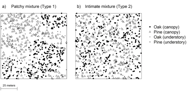
(2006). The first type of mixture is characterized by monospecific clusters (clusters of oaks 81
and clusters of pines) with interspecific spatial repulsion (Fig. 1a). For this first type, 82
repulsion occurs between clusters of individuals. This "patchy mixture" is henceforth called 83
Type 1. In the second type of mixture, individual oaks and pines are randomly scattered (or 84
only slight aggregated) (Fig. 1b). Here, the interspecific structure is characterized by 85
repulsion between individuals at short distances and results in an intimate mixture at the plot 86
scale. This “intimate mixture” is referred to as Type 2 in the following sections. 87
We also took the understory trees into account since they participate in stand productivity and 88
are involved in local competition. In the studied stands, the understory is mainly composed of 89
oak. Several types of spatial pattern have been identified for the understory in these stands 90
(Ngo Bieng 2007). However, in eight of the nine plots where we measured tree growth, the 91
spatial pattern of the understory was the same. Consequently, we chose only one type of 92
spatial pattern for the understory and applied it to both types of mixture (Type 1 and Type 2). 93
2.2 Point process models of oak-pine mixed stands.
94
2.2.1Point process models
95
The point process model we used in our study was a combination of classic point processes. 96
In forestry applications, as in this study, the spatial pattern of the trees in a stand is assumed to 97
result from a given point process. We therefore used known point processes to reproduce the 98
spatial features observed in the studied stands. In order to generate clustered or aggregated 99
spatial point patterns, we used the Neyman-Scott (NS) point process (Tomppo 1986; Ngo 100
Bieng et al. 2011). In order to generate the repulsion between individuals or groups of 101
individuals, we used the “soft core” (SC) point process, which is a pairwise interaction 102
process where pairs of points should not be closer than a threshold distance or “soft core” 103
distance (Illian et al. 2008; Ngo Bieng et al. 2011). With the combination of these two point 104
processes, Ngo Bieng et al. (2011) developed point process models fitted on field data to 105
reproduce the spatial patterns of oak-pine mixed stands. These models took into account the 106
spatial pattern of the two species when reproducing the observed spatial features, thus 107
describing the spatial interactions between qualitative marks associated to the simulated 108
spatial point process. For our work, we used the point process models developed by Ngo 109
Bieng et al. (2011) to simulate oak-pine mixed stands. These models are described in the 110
following subsections. 111
2.2.2Point process model for spatial pattern of Type 1: patchy mixture 112
This point process model is a combination of Neyman-Scott processes (NS) and soft core 113
processes (SC). Oak locations were simulated by an NS process. Pines locations were 114
simulated by a NS process with an additional regularity constraint obtained through a SC 115
process. The regularity constraint takes into account regularity at short distances, which is 116
typical of the spatial pattern of pines (Ngo Bieng 2006). The regularity constraint is a 117
threshold distance of regularity (dreg) which corresponds to the minimum distance allowed 118
between two pines. To generate a more realistic regularity, if the distance between two pines 119
is below the threshold distance, tree locations can be retained with a probability depending on 120
the distance between the two trees (principle of the SC process). This probability varies 121
linearly from 0 at a null distance to 1 at the threshold distance dreg. Interspecific repulsion 122
was also simulated with a SC process and a repulsion distance drep. The Type 1 model has 123
six parameters (Table 2): the number of oak aggregates (ncloak), the radius of the oak
124
aggregates (rcloak), the number of pine aggregates (nclpine), the radius of pine aggregates
125
(rclpine), the minimal intraspecific distance between pines or regularity distance (dreg), the
126
minimal repulsion distance between oaks and pines or repulsion distance (drep). 127
2.2.3Point process model for spatial pattern of Type 2: intimate mixture 128
This model is a combination of a NS process and a SC process. Pine locations were simulated 129
with a NS process with a regularity constraint obtained with a SC process as explained for the 130
previous model. Oak individuals were then randomly simulated with a repulsion distance also 131
ensured with a SC process. Contrary to the previous model, the probability of accepting an 132
oak closer to a pine than the threshold repulsion distance is constant and does not vary with 133
the distance. This model has five parameters (Table 2): the number of pine aggregates 134
(nclpine), the radius of pine aggregates (rclpine), the intraspecific minimal distance between
135
pines or distance of regularity (dreg), the minimal repulsion distance between oaks and pines 136
(drep) and p the constant probability to accept an oak tree at a distance lower than drep from a 137
pine. 138
2.2.4 Point process model for oak understory 139
As mentioned previously, the understory was mainly composed of oak, and its spatial pattern 140
did not vary much among the studied plots. We therefore chose to simulated only one type of 141
spatial pattern for understory oaks: the most frequent type in the plots where growth was 142
measured. For Type 1 and Type 2 mixtures, the simulated spatial pattern of understory oaks 143
was therefore identical. As we did for the canopy trees, we used a point process model fitted 144
on field data to simulate the locations of understory oaks (Ngo Bieng et al. 2011). This point 145
process model simulates an attraction with the oaks in the canopy and a repulsion with the 146
pines in the canopy. The point process model for the understory oaks was a combination of 147
NS and SC processes. First, understory oaks were simulated with a NS process. During this 148
simulation, repulsion with the pines in the canopy was ensured with a SC process containing 149
an additional constraint of attraction with canopy oaks. This attraction constraint between 150
understory and canopy oaks was simulated by checking that each understory oak was at a 151
distance below or equal to a given attraction distance. This model had four parameters (Table 152
2): the number of oak aggregates in the understory (nclund), the radius of oak aggregates in the
153
understory (rclund), the distance of intraspecific attraction between understory oaks and
154
canopy oaks (dattr), the distance of interspecific repulsion between understory oaks and 155
canopy pines (drep). 156
Fig. 1 presents simulated stands for the patchy (Type1) and the intimate (Type2) mixtures. 157
2.3Spatially explicit individual growth models
158
As mentioned above, we developed our growth model from data collected from nine plots in 159
the Orleans forest. The nine plots cover the two types of mixture simulated in this work 160
(Table 1). In each plot, we selected 30 oaks and 30 pines based on a stratified sampling 161
method. The stratification variables were tree size and local environment (see Perot et al. 162
2010 for details). Sampled trees were cored to the pith at a height of 1.3 m. The cores were 163
scanned and analyzed using the WinDENDRO software, version 2005a (Regent 2005), and 164
ring width was measured to the nearest 0.01 mm. The COFECHA software (Grissino-Mayer 165
2002) was used to cross-date the individual ring-width series. The ring width analyses were 166
performed on a final total of 230 oaks and 269 pines. Detailed information on past 167
disturbances was not available for our plots (location and size of suppressed trees) so we 168
chose the 6 years period from 2000 to 2005 to study tree growth because there had been no 169
thinnings or storms during that time. 170
The growth model we developed is a spatially explicit individual based model based on local 171
competition indices (Uriarte et al. 2004b). This model is similar to that presented by Perot et 172
al. (2010) but for the present study we added a plot random effect to account for factors 173
influencing tree growth at the plot level (soil quality, stand age, stand density). The final 174
model for each species was a linear mixed effect model. For both species, the competition 175
indices were the basal areas of the oaks and pines belonging to the neighborhood of the target 176
tree (CIoak et CIpine). In a previous work on the same plots (Perot et al. 2010), several radii (5,
177
10 and 15m) were tested for the neighborhood so as to cover the range of radii reported in 178
other studies (Canham et al., 2004; Stadt et al., 2007; Uriarte et al., 2004a) and to minimize 179
the influence of edge effects when computing the competition indices. Based on model 180
comparisons, the authors concluded that indices computed with a 10 m radius gave the best 181
results. Based on this work, we defined the neighborhood as a 10 m radius circle around the 182
target tree. These competition indices account for both intra- and interspecific competitions. 183
For each species the final model was written as follows: 184
(
) (
)
, 0 0 , oak ,oak pine , pine ,
i k k k i k i i i k
r α α β β girth λ CI λ CI ε
∆ = + + + + + + (1)
185
where ∆ri,k is the radial increment of tree i for plot k over a growth period of 6 years, girthi,k is
186
the girth of tree i at 1.3 m, CIi,oak and CIi,pine are the competition indices for oak competitors
187
and pine competitors respectively, {α0, β0, λoak, λpine} are the parameters estimated for the
188
fixed effects of the model, {αk, βk} are the parameters corresponding to the random part of the
189
model (plot effect) and εi,k is the residual part of the model.
190
Preliminary results showed that the variance of the residuals increased with the adjusted 191
values. To correct for this heteroscedasticity, we modeled the variance of the residuals with 192
the fitted values and a power function (Eq. 2), as suggested by Pinheiro and Bates (Pinheiro 193
and Bates 2000): 194
Var(εi,k) = σ2|(fitted valuei,k)|2δ (2)
Where δ is the parameter of the variance model. The model was fitted using the R software 196
version 2.14.0 (R Development Core Team 2011) with the lme function of the nlme package 197
(Pinheiro et al. 2011). 198
2.4Simulation experiment design
199
Initial stands for the two types of mixture were simulated with the point process models 200
presented in section 2.2. Since stand density and tree size influence individual growth (see Eq. 201
1), in order to have exactly the same number of trees of each species and exactly the same 202
dendrometric characteristics for the two types of mixture, we used the same tree list to 203
simulate the initial stands for both mixture types. With this method, we ensured that the only 204
parameter that changed between Type 1 and Type 2 mixtures was the spatial pattern of the 205
trees. We carried out our simulations on a 1-ha plot (Table 4). 206
Both the spatial pattern within a mixture and growth show some variability. This variability 207
was estimated from field data and was included in the point process models as well as in the 208
individual growth model. To account for the different sources of variability, it was necessary 209
to carry out several simulations with each model. We proceeded as follows: a) to account for 210
variability in the spatial pattern within a mixture type, each type was simulated 200 times, b) 211
to account for growth variability at the plot level, for each initial stand the parameters αk et βk
212
(Equation 1) were simulated 50 times, c) to account for variability in individual growth 213
(residual variability), for each initial stand and each pair of values {αk, βk}, individual tree
214
growth was simulated 10 times following Equation 1. In all, we performed 200,000 215
simulations (2 * 200 * 50 * 10). For each simulation, we calculated the basal area productivity 216
for oak and for pine. All the simulations were performed in the Capsis platform with the 217
oakpine1 module (Dufour-Kowalski et al. 2012). 218
2.5Decomposition of the basal area productivity variability
219
Thanks to our simulation design, we were able to estimate the effects of several factors on the 220
productivity of both species: 1) an effect related to the type of mixture, 2) an effect related to 221
the variability in the spatial pattern within the type of mixture, 3) an effect related to the 222
growth variability between plots (plots are nested in the type of mixture) and 4) an effect 223
related to tree growth variability within the plot: 224
ijkl i ij ijk ijkl
y = +µ type +pp + plot +ε (3)
225
Where yijkl is the basal area productivity of one species, µ is the general mean, typei is the type
226
of mixture effect, ppij is the spatial pattern random effect in the type, plotijk is the plot random
227
effect of the growth model in each point process realization, εijkl is the residual and
228
corresponds to tree level variability in the growth model. The structure of our simulation 229
design (balanced nested design) made it possible to decompose the variability of species 230
productivity into different components and to estimate the contribution of each component to 231
variability as follows (for simplicity, the variance σ2 and the estimate of the variance are 232 denoted identically): 233
(
)
(
) (
)
(
) (
)
2 2 2 2 2 2 2 2 2 2 2 2 2 2 2 with res resplot plot res res
total type pp plot res
pp pp res res plot res plot
type type res res plot res plot pp res plot pp
MSD MSD n MSD n n n MSD n n n n n n
σ
σ
σ
σ
σ
σ
σ
σ
σ
σ
σ
σ
σ
σ
σ
= = − = + + + = − − = − − − 234Where MSD is the mean square deviation for the different sources of variability, ntype = 2, npp
235
= 200, nplot = 50, and nres = 10. We then assessed the importance of spatial pattern variability
236
in the productivity variability of each species. The sum of
σ
type2 and2
pp
σ
was considered to be 237the overall contribution of spatial pattern to productivity variability. 238
3.
Results
239The results of the growth model show that, for oak, the effect of oak competition on growth is 240
about twice higher than the effect of pine competition (see λoak and λpine in Table 3). The
241
magnitude of the effect of pine competition on pine growth is close to the effect of pine 242
competition on oak growth (-0.085 mm.m-2 and -0.094 mm.m-2 respectively). But contrary to 243
oak, the competition index computed on oaks has no significant effect on pine growth. 244
The results of the simulations show that productivity in Type 2 (intimate mixture) is higher 245
than in Type 1 (patchy mixture) for both species (Fig. 2). The difference in productivity 246
between Type 2 and Type 1 is more pronounced for oak than for pine: +14.7% for oak and 247
+11.3% for pine. 248
The productivity values obtained for oak and pine show some variability. If we combine the 249
results from the two types of mixture, oak productivity varies from 0.23 to 0.36 m².ha-1.year-1 250
(first and ninth deciles) with a coefficient of variation of 0.175 (ratio of the standard deviation 251
to the mean). Pine productivity varies from 0.19 to 0.35 m².ha-1.year-1 (first and ninth deciles) 252
with a coefficient of variation of 0.228. Variability in pine productivity is thus slightly higher 253
than that of oak. 254
The results also show that most of the productivity variability is explained by plot effect, 255
which represents 86% of the total variability for pine and 67% for oak (Fig. 3). The spatial 256
pattern (type of spatial pattern + random effect in the type) explains 12% of the variability for 257
pine and 31% for oak. The overall effect of spatial pattern on oak productivity is important. 258
Even if the individual growth variability within a plot is high, it has little impact on the 259
overall productivity variability (between 1 and 2% of the total variability). Variability in 260
spatial pattern within a mixture type also has a relatively little impact, though the effect on 261
oak productivity (5%) is slightly higher than on pine productivity (2%). 262
4.
Discussion
2634.1 Spatial pattern and species productivity
264
Spatial pattern plays a key role in the interactions between species in plant communities 265
(Dieckmann et al. 2000). These interactions influence ecological processes involved in the 266
species dynamics: growth, regeneration and mortality (Begon et al. 2006). Our results show 267
that the productivity of sessile oak and Scots pine is higher in an intimate mixture (Type 2) 268
than in a patchy mixture (Type 1). Our work has made it possible to estimate the difference in 269
species basal area productivity between the two types of mixture. This difference was 11.3% 270
for pine and 14.7% for oak (Fig. 2). These figures are comparable to those of Pukkala (1989) 271
who simulated Scots pine productivity in pure stands for different spatial patterns. He found 272
that volume productivity was 10% lower in aggregated spatial patterns compared to regular 273
spatial patterns. Our results also show that the plot effect explains a large part of the 274
productivity variability (Fig. 3). The plot effect, estimated with the growth model, includes 275
several factors that affect tree growth: (i) a site effect - soil conditions vary from one plot to 276
another and affect species productivity, (ii) an age effect - young stands have higher 277
productivity and finally, (iii) a density effect - denser stands generally have higher 278
productivity (Vallet and Perot 2011). The variability obtained for pine productivity is similar 279
to that of oak productivity but is much more influenced by plot effects (Fig. 3). 280
4.2 Influence of spatial and growth interactions
281
Intra- and interspecific competition are crucial to understand the effect of mixture on forest 282
productivity and forest dynamic (Kelty 2006; Forrester et al. 2006). As in the study of Perot et 283
al. (2010), our results showed that, for both species, intraspecific competition had a more 284
negative effect on growth than interspecific competition (see parameters λoak and λpine in Table
285
3). Oak had little impact on pine growth probably because pines had a greater girth than oaks 286
on average (Table 1). The light interception by the pine foliage is lower than the light 287
interception by the oak foliage (Balandier et al. 2006; Sonohat et al. 2004). This may help to 288
explain that in our oak model, the interspecific competition was lower than the intraspecific 289
competition. The two species involved have different light requirements but also different 290
root distribution patterns (Brown 1992). The complementarity in nutrient and water use could 291
also contribute to explain why intraspecific competition was more severe than interspecific 292
competition. The local competition and the spatial features of each mixture type help to 293
explain the results of this work. Two spatial features vary simultaneously between Types 1 294
and 2: the intraspecific pattern and the interspecific pattern. Ripley's function and inter-type 295
function (Ripley 1977; Lotwick and Silverman 1982; Perot and Picard 2012) can be used to 296
characterized and compare these two dimensions. On average in the patchy mixture (Type1), 297
there are more oaks around an oak tree than in the intimate mixture (Type 2) (see L functions 298
at 10 m for oak in Fig. 4). Consequently, the competition index ICoak is higher, on average, in
299
Type 1 than in Type 2. In contrast, in Type 1 mixture, there are fewer pines on average around 300
an oak tree than in Type 2 (see inter-type functions at 10 m in Fig. 4). Consequently, the 301
competition index ICpine is lower, on average, in Type 1 than in Type 2. In addition, the
302
parameters of the growth model must be examined. Parameters λoak and λpine (Table 3) show
303
that oak competitors (ICoak) have a more negative effect on oak growth than do pine
304
competitors (ICpine) (λoak is more negative than λpine). In the intimate mixture (Type 2) there
305
are more pines around oaks than in the patchy mixture (Type 1) and pines are less competitive 306
than oaks. This explains why oak productivity is higher, on average, in the intimate mixture 307
than in the patchy mixture. For one particular simulation, the final result is complex because 308
productivity depends on both intra- and interspecific competition (estimated through 309
parameters λoak and λpine) and also on intra- and interspecific spatial patterns. Variability in the
310
spatial pattern of a mixture type thus explains why oak productivity in Type 2 is not always 311
higher than in Type 1 (Fig. 2). The reasoning is similar for pine but the result is easier to 312
analyze because there is no interspecific competition parameter in the individual growth 313
model. For pine, productivity depends only on the intraspecific spatial pattern. 314
4.3 Influence of species assemblage and stand age
315
The effect of spatial pattern on species productivity in mixed stands should depend on species 316
assemblage. In our study, both oak and pine were favored in the intimate mixture because, for 317
both species, intraspecific competition was more severe than interspecific competition. Other 318
authors have also shown that interspecific competition was lower than intraspecific 319
competition (e.g. Forrester and Smith 2012), while some studies have shown the opposite in 320
some conditions (e.g. Pretzsch et al . 2010). Intensity of interactions may also change with 321
species assemblages. Further works involving other species are therefore necessary to 322
generalize our results. Moreover, for tree species, the competition relationship between 323
species may depend on stand developmental stage (Filipescu and Comeau 2007; Cavard et al. 324
2011). Pine is a fast growing species compared to oak (Duplat and Tran-Ha 1997; Perot et al. 325
2007). In young stage, pine is probably more competitive than oak. Consequently, oak 326
productivity could be favored by a patchy mixture at an earlier stage. In addition, Getzin et al. 327
(2006) showed that interspecific competition is less intense at older stages than at younger 328
stages, probably due to the spatial sharing of resources. In our study, this would explain why 329
the mixture type had less impact on pine productivity than on oak productivity, and why pine 330
is more influenced by plot effects (site, age, density) than oak. 331
Conclusion
332
Our study is innovative in that we worked on a mature mixed forest. For such complex 333
forests, models and simulations can provide interesting quantitative results that would be 334
difficult to obtain through experimentation. The two mixture types that we tested are realistic 335
oak-pine mixtures found in central France (Ngo Bieng et al. 2006). Our results show that their 336
spatial differences are contrasted enough to have an impact on the productivity of both species 337
in the mixture. From a practical point of view, our work shows the interest of favoring 338
intimate mixtures in mature oak-pine stands to optimize tree species productivity. Oak is the 339
species that benefits most from this type of management. In order to achieve more general 340
results, further work is needed to determine the change in competition between oak and pine 341
over time. 342
5.
Acknowledgments
343This work forms part of the PhD traineeships of M. A. Ngo Bieng and T. Perot and was 344
funded in part by the research department of the French National Forest Office. We are 345
grateful to the Loiret agency of the National Forest Office for allowing us to install the 346
experimental sites in the Orléans state forest. Many thanks to the Irstea staff at Nogent-sur-347
Vernisson who helped collect the data: Fanck Milano, Sandrine Perret, Yann Dumas, 348
Sébastien Marie, Romain Vespierre, Grégory Décelière. Many thanks to Victoria Moore for 349
her assistance in preparing the English version of the manuscript. 350
351
6.
References
352Balandier P, Sonohat G, Sinoquet H, Varlet-Grancher C, Dumas Y (2006) Characterisation, 353
prediction and relationships between different wavebands of solar radiation 354
transmitted in the understorey of even-aged oak (Quercus petraea, Q-robur) stands. 355
Trees-Struct Funct 20 (3):363-370 356
Barot S, Gignoux J, Menaut JC (1999) Demography of a savanna palm tree: Predictions from 357
comprehensive spatial pattern analyses. Ecology 80 (6):1987-2005 358
Begon M, Townsend CR, Harper JL (2006) Ecology: from indivuals to ecosystems. 4th ed. 359
Blackwell Publishing, Oxford 360
Canham CD, LePage PT, Coates KD (2004) A neighborhood analysis of canopy tree 361
competition: effects of shading versus crowding. Can J For Res 34 (4):778-787 362
Cavard X, Bergeron Y, Chen HYH, Paré D, Laganière J, Brassard B (2011) Competition and 363
facilitation between tree species change with stand development. Oikos 120 364
(11):1683-1695 365
Courbaud B, Goreaud F, Dreyfus P, Bonnet FR (2001) Evaluating thinning strategies using a 366
tree distance dependent growth model: some examples based on the CAPSIS 367
software "uneven-aged spruce forests" module. For Ecol Manag 145 (1-2):15-28 368
Cressie NAC (1993) Statistics for spatial data. John Wiley and sons, New York 369
Dieckmann U, Law R, Metz JAJ (2000) The Geometry of Ecological Interactions: 370
Simplifying Spatial Complexity. Cambridge University Press, Cambridge 371
Dufour-Kowalski S, Courbaud B, Dreyfus P, Meredieu C, de Coligny F (2012) Capsis: an 372
open software framework and community for forest growth modelling. Ann For Sci 373
69 (2):221-233 374
Duplat P, Tran-Ha M (1997) Modélisation de la croissance en hauteur dominante du chêne 375
sessile (Quercus petraea Liebl) en France Variabilité inter-régionale et effet de la 376
période récente (1959-1993). Ann For Sci 54 (7):611-634 377
Filipescu CN, Comeau PG (2007) Competitive interactions between aspen and white spruce 378
vary with stand age in boreal mixedwoods. For Ecol Manag 247 (1-3):175-184 379
Forrester DI, Bauhus J, Cowie AL, Vanclay JK (2006) Mixed-species plantations of 380
Eucalyptus with nitrogen-fixing trees: A review. For Ecol Manag 233 (2-3):211-230 381
Forrester DI, Smith RGB (2012) Faster growth of Eucalyptus grandis and Eucalyptus pilularis 382
in mixed-species stands than monocultures. For Ecol Manag 286:81-86 383
Getzin S, Dean C, He FL, Trofymow JA, Wiegand K, Wiegand T (2006) Spatial patterns and 384
competition of tree species in a Douglas-fir chronosequence on Vancouver Island. 385
Ecography 29 (5):671-682 386
Grissino-Mayer HD (2002) Research report evaluating crossdating accuracy: a manual and 387
tutorial for the computer program COFECHA. Tree-Ring Research 57 (2):205-221 388
Illian J, Penttinen A, Stoyan H, Stoyan D (2008) Statistical Analysis and Modelling of Spatial 389
Point Patterns. Wiley, Chichester 390
Jactel H, Brockerhoff EG (2007) Tree diversity reduces herbivory by forest insects. Ecol Lett 391
10 (9):835-848 392
Kelty MJ (2006) The role of species mixtures in plantation forestry. For Ecol Manag 233 (2-393
3):195-204 394
Lamosova T, Dolezal J, Lanta V, Leps J (2010) Spatial pattern affects diversity-productivity 395
relationships in experimental meadow communities. Acta Oecol-Int J Ecol 36 396
(3):325-332 397
Lenoir J, Gégout JC, Marquet PA, de Ruffray P, Brisse H (2008) A significant upward shift in 398
plant species optimum elevation during the 20th century. Science 320 (5884):1768-399
1771 400
Lotwick HW, Silverman BW (1982) Methods for analysing spatial processes of several types 401
of points. Journal of the Royal Statistical Society B 44 (3):406-413 402
McNaughton SJ (1977) Diversity and stability of ecological communities - comment on role 403
of empiricism in ecology. Am Nat 111 (979):515-525 404
MCPFE, UNECE, FAO (2011) State of Europe's forests 2011. MCPFE, Warsaw 405
Mokany K, Ash J, Roxburgh S (2008) Effects of spatial aggregation on competition, 406
complementarity and resource use. Austral Ecol 33 (3):261-270 407
Ngo Bieng MA (2007) Construction de modèles de structure spatiale permettant de simuler 408
des peuplements virtuels réalistes. Application aux peuplements mélangés Chêne 409
sessile - Pin sylvestre de la région Centre. Doctorat thesis in Forestry Science, 410
ENGREF-Cemagref, Nogent-sur-Vernisson 411
Ngo Bieng MA, Ginisty C, Goreaud F (2011) Point process models for mixed sessile forest 412
stands. Ann For Sci 68 (2):267-274 413
Ngo Bieng MA, Ginisty C, Goreaud F, Perot T (2006) A first typology of Oak and Scots pine 414
mixed stands in the Orleans forest (France), based on the canopy spatial structure. N 415
Z J For Sci 36 (2):325-346 416
Perot T, Goreaud F, Ginisty C, Dhôte JF (2010) A model bridging distance-dependent and 417
distance-independent tree models to simulate the growth of mixed forests. Ann For 418
Sci 67 (5):502p501-502p511 419
Perot T, Perret S, Meredieu C, Ginisty C (2007) Prévoir la croissance et la production du Pin 420
sylvestre : le module Sylvestris sous Capsis 4. Revue Forestiere Francaise 59 (1):57-421
84 422
Perot T, Picard N (2012) Mixture enhances productivity in a two-species forest: evidence 423
from a modelling approach. Ecol Res 27:83-94 424
Pinheiro JC, Bates DM (2000) Mixed-effects models in S and S-PLUS. Statistics and 425
Computing. Springer, New York 426
Pinheiro JC, Bates DM, DebRoy S, Sarkar D, the R Development Core Team (2011) nlme: 427
linear and nonlinear mixed effects models. R package version 3.1-101. 428
Pretzsch H (1997) Analysis and modeling of spatial stand structures. Methodological 429
considerations based on mixed beech-larch stands in Lower Saxony. For Ecol Manag 430
97 (3):237-253 431
Pretzsch H, Schutze G (2009) Transgressive overyielding in mixed compared with pure 432
stands of Norway spruce and European beech in Central Europe: evidence on stand 433
level and explanation on individual tree level. Eur J For Res 128 (2):183-204 434
Pretzsch H, Block J, Dieler J, Hoang Dong P, Kohnle U, Nagel J, Spellmann H, Zingg A 435
(2010) Comparison between the productivity of pure and mixed stands of Norway 436
spruce and European beech along an ecological gradient. Ann For Sci 67 (7):712 437
Pukkala T (1989) Methods to describe the competition process in a tree stand. Scand J Forest 438
Res 4:187-202 439
R Development Core Team (2011) R: A language and environment for statistical computing. 440
R Foundation for Statistical Computing, Vienna, Austria 441
Regent I (2005) Windendro 2005a: manual for tree-ring analysis. Université du Quebec à 442
Chicoutimi 443
Ripley BD (1977) Modelling spatial patterns. Journal of the royal statistical society B 39:172-444
212 445
Sonohat G, Balandier P, Ruchaud F (2004) Predicting solar radiation transmittance in the 446
understory of even-aged coniferous stands in temperate forests. Ann For Sci 61 447
(7):629-641 448
Stadt KJ, Huston C, Coates KD, Feng Z, Dale MRT, Lieffers VJ (2007) Evaluation of 449
competition and light estimation indices for predicting diameter growth in mature 450
boreal mixed forests. Ann For Sci 64:477-490 451
Tomppo E (1986) Models and methods for analysing spatial patterns of trees. 452
Communicationes Instituti Forestalis Fenniae (No. 138) 453
Uriarte M, Canham CD, Thompson J, Zimmerman JK (2004a) A neighborhood analysis of 455
tree growth and survival in a hurricane-driven tropical forest. Ecol Monogr 74 456
(4):591-614 457
Uriarte M, Condit R, Canham CD, Hubbell SP (2004b) A spatially explicit model of sapling 458
growth in a tropical forest: does the identity of neighbours matter? J Ecol 92 (2):348-459
360 460
Vallet P, Perot T (2011) Silver fir stand productivity is enhanced when mixed with Norway 461
spruce: evidence based on large-scale inventory data and a generic modelling 462
approach. J Veg Sci 22 (5):932-942 463
Vanclay JK (2006) Experiment designs to evaluate inter- and intraspecific interactions in 464
mixed plantings of forest trees. For Ecol Manag 233 (2-3):366-374 465
Vettenranta J (1999) Distance-dependent models for predicting the development of mixed 466
coniferous forests in Finland. Silva Fenn 33 (1):51-72 467
468 469 470
23
7.
Tables
Table 1: Dendrometric characteristics of the nine plots used for growth models (Orléans Forest, France). BA = basal area; Other = other broadleaf tree species; D = mean diameter at a height of 130 cm; Age = mean age of the cored trees at a height of 130 cm; Ho = dominant height. Only the height of the sample trees was measured. The dominant height was estimated with a measure of the dominant diameter and a height-diameter relationship fitted for each species and each plot using the sample trees; PP = type of spatial pattern, 1 = patchy mixture, 2 = intimate mixture, 3 = intermediate type with cluster of pines and oaks randomly scattered; For diameters and ages, values represent the mean with the standard deviation in parentheses.
Plot Area (ha) BAoak (m².ha-1) BApine (m².ha-1) BAother (m².ha-1) BAtotal (m².ha-1) Doak (cm) Dpine (cm)
Ageoak Agepine Hooak
(m) Hopine (m) PP P108 0.80 9.6 19.8 1.4 30.8 17.7 (6.74) 36.2 (5.31) 68 (4.3) 66 (2.5) 22.3 23.0 2 P178 1.00 16.5 10.0 1.5 28.0 21.5 (10.49) 36.5 (7.56) 78 (4.6) 77 (1.8) 21.1 22.1 1 P184 0.75 10.9 12.0 2.1 25.1 17.5 (8.88) 36.3 (7.76) 71 (8.6) 68 (4.2) 21.9 20.8 3 P216 0.50 11.2 12.1 0.9 24.1 17.0 (6.39) 27.8 (7.6) 52 (2.8) 50 (2.2) 18.8 19.0 2 P255 1.00 12.6 10.5 1.1 24.2 17.8 (7.54) 31.7 (6.25) 69 (5.9) 62 (4.6) 20.1 19.7 2 P534 0.50 12.2 19.6 1.0 32.7 16.6 (6.54) 37.4 (6.5) 59 (2.3) 83 (3.2) 22.1 22.5 2 P563 0.50 13.6 11.9 0.2 25.7 25.1 (10.12) 35.6 (4.58) 70 (3.1) 69 (2.3) 24.5 23.0 2 P57 1.00 11.2 11.4 0.4 23.0 16.7 (6.36) 34.3 (6.41) 67 (7.1) 62 (3.1) 20.4 21.2 1 P78 0.70 14.7 16.5 1.0 32.2 20.1 (7.48) 42.2 (8.79) 62 (5.2) 112 (17.5) 21.8 25.6 2
24
Table 2 Parameters in the point process models. nclsp = number of aggregates for species sp; rclsp = radius of aggregates for species sp; dreg = distance of regularity which corresponds to the minimum distance allowed between pines; drep = repulsion distance between oaks
and pines; und = oak understory; dattr = distance of intraspecific attraction between understory oaks and canopy oaks.
Parameters in the point process model Species Tree position Type of spatial pattern nclpine
(ha-1) rclpine (m) dreg (m) ncloak (ha-1) rcloak (m) drep (m)
Oak and pine Canopy Type 1 (Patchy mixture) 13 18 5 7 17 18
nclpine (ha-1) rclpine (m) dreg (m) drep (m) p
Oak and pine Canopy Type 2 (Intimate mixture) 38 8 10 4 0.15
nclund (ha-1) rclund (m) dattr (m) drep (m)
25
Table 3 Parameter estimates of the spatially explicit individual growth model (see Eq. 1).
Parameter estimates Model statistics
Intercept α (mm) girth β (mm.cm-1) CIoak λoak (mm.m-2) CIpine λpine (mm.m-2) δa RSE df AIC Oak Estimates 3.335 0.126 -0.196 -0.094 0.526 1.013 218 1196 Std. error 1.202 0.018 0.042 0.024 P-value 0.006 <0.001 <0.001 <0.001 σplot 2.036 0.048 Pine Estimates 2.711 0.0654 -0.0855 0.621 0.838 258 1413 Std. error 1.054 0.0094 0.0241 P-value 0.011 <0.001 <0.001 σplot 0.0145 a
26
Table 4 Dendrometric features of the initial stand used in simulations (stand area = 1 ha). For girth, the value in parentheses corresponds to the standard deviation.
Number of trees Girth (cm)
Species Canopy Understory mean min. max.
Oak 284 208 53.2 (23.2) 23 129
27
8.
Figure captions
Fig. 1 a) Patchy mixture (Type 1) simulated with the point process models; b) Intimate mixture (Type 2) simulated with the point process models.
28 Fig. 2 Productivity comparison between the two mixture types for oak and pine.
29 Fig. 3 Decomposition of the productivity variability for oak and pine following Equation (3). The different sources of variability are: type of mixture (Type), spatial point pattern within the type (PP), plot random effect (Plot), and tree random effect (Tree).
30 Fig. 4 L function and intertype L function calculated with 1000 simulations of Type 1 and Type 2 mixtures. For the intraspecific L function, L(r) less than 0 indicates spatial regularity, L(r) greater than 0 indicates spatial aggregation. For the intertype L
function, L(r) less than 0 indicates spatial repulsion between the two species, L(r) greater than 0 indicates spatial attraction between the two species.