Analysis of hunting in Synchronous Hysteresis Motor

Analysis of Hunting in Synchronous Hysteresis Motor by

Cang Kim Truong

Submitted to the Department of Electrical Engineering and Computer Science in Partial Fulfillment of the Requirements for the Degrees of

Master of Engineering in Electrical Engineering and Computer Science at the

Massachusetts Institute of Technology February 2004

Copyright 02004 Cang Kim Truong. All rights reserved. The author hereby grants to M.I.T. permission to reproduce and

distribute publicly paper and electronic copies of this thesis and to grant others the right to do so.

MASSACHUSETTS INSTI E OF TECHNOLOGY

JUL 2 0 2004

LIBRARIES

Departm r of Electrical Engineering d"Computer Science

January 30, 2004

Certified by

Jonathan Cole Principle Member of the Technical Staff, The Charles Stark Draper Laboratory

Certified by

James Kirtley

Professor o4 Fectrical Engineering

Accepted by

Ahur C. Smith

Analysis of Hunting in Synchronous Hysteresis Motor by

Cang Kim Truong Submitted to the

Department of Electrical Engineering and Computer Science February 2004

In Partial Fulfillment of the Requirements for the Degree of Master of Engineering in Electrical Engineering and Computer Science

ABSTRACT

The Synchronous Hysteresis Motor has an inherent instability when it is used to drive a gyroscope wheel. The motor ideally should spin at a constant angular velocity, but it instead sporadically oscillates about synchronous speed. This phenomenon is known as 'hunting'. This problem produces current ripples at the motor's electrical terminals and induces noise on the sensors that monitor gyro activity. This thesis examines the cause of hunting by deriving the motor's torque characteristics from first principles. It also derives a scheme for suppressing hunting by monitoring the motor's current as an indicator of drag angle and using it to modulate the motor's drive frequency. Explanation of the circuit that successfully implements this scheme is included and lab results are shown to verify the working theory.

Thesis Supervisor: Penn Clower

Title: Principle Member of the Technical Staff, The Charles Stark Draper Laboratory Thesis Advisor: Professor James Kirtley

ACKNOWLEDGMENTS January 30, 2004

This thesis was prepared at The Charles Stark Draper Laboratory, Inc., under contract N00030-02-C-0006, account 50-17199.

Publication of this thesis does not constitute approval by Draper or the sponsoring agency of the findings or conclusions contained herein. It is published for the exchange and stimulation of ideas.

I am forever grateful to Penn Clower for being my mentor at Draper and giving me the idea for this thesis. His demeanor, philosophy, and leadership have helped me mature tremendously as an engineer. After I spent a couple of summers with Penn, his lessons facilitated my understanding of the course material at MIT. He is a treasure trove of stories and fascinating facts, always teaching those around him the various phenomena of this world. He organizes informal chats at the lab and he makes a tradition of rallying us up to climb Mt. Monadnock every year. Penn, you are a huge benefit to my life and your spirit lives in me. I find that I also rally up folks around me to go on outings. Many

come to me for technical advice, and some of the answers I attribute to you.

I want to also thank my faculty advisor Professor Kirtley for giving Penn and me ideas when we were at a dead end. His hysterical sense of humor and mischievous smile made the struggle an enjoyable undertaking. His teaching provided insight about the thesis and it helped with the analysis.

I want to especially thank my favorite personality at MIT, Ron Roscoe. His analog death lab gave me the hands-on skill to debug circuits. Anyone who takes his class comes out an able engineer, capable of building any kind of gadget using analog components. He contributed the most value to my MIT experience.

I want to mention my parents, Vinh Truong and Hay Nguyen, who are the main reasons I live. When I was a child, they carried me atop their backs through the rain, sun, moon, stars, and even gunfire across Vietnam's swamps on our adventure to America. Because of their struggle, I am undeniably happy every day of my existence. As an adult, I look toward the opportunity to carry them on my back.

My sisters, Vi, Uyen, and Lana, have urged me on throughout my life. Their unconditional loyalty is the quality I incessantly seek in others.

I am honored to have shared happy times with MIT's super geniuses: Hoeteck Wee, Hiro Iwashima, Zhenye Mei, Yao Li, Mamat Rachmat Kaimuddin, Sendokan Thevendran, Radhika Baliga, Rahul Agrawal, Esosa Amayo, Satapom Pornpromlikit, Bua, Aina, Lily Huang, Louise Giam, and Hanwei Li. Their friendship taught me that relationships are bound by the heart and its irrationality, not reason. Good times!!!

Lastly, thank you Alan Wu, Jon Cole, Keith Baldwin, and Joan Orvosh for your support during my fellowship at Draper.

CONTENTS

Introduction to the Problem ... 7

R elated W orks ... 8

Thesis Goals and Approach ... 10

T hesis O utline ... 11

Motor Topology and Basic Operation ... 12

Energy, the Link from Flux to Torque ... 16

M otor A ssum ptions ... 20

Flux Linkage Derivation ... 21

Flux Linkage Approximation ... 27

Motor Torque Expression ... 28

Motor Dynamic Behavior ... 32

Second Order Effects on Drag Angle 0 ... 35

Comparing Analytical Expression with Lab Results ... 40

Chapter 4: Bridging Analysis with Empirical Measurements ... 42

Chapter 5: 5.1 5.2 5.3 5.4 5.5 Scheme for Damping the Hunting ... 45

FM Modulation Chosen Over AM ... 46

Hunting Suppression Implementation ... 47

The Control Circuit ... 51

Circuit Schematic Elaboration ... 53

L ab R esults ... 56

Chapter 6: Conclusion ... 59

6.1 Further Investigation Possibilities ... 59

Appendix A: Modeling the Hysteresis Motor in Simulink ... 61

Figures

Figure 1: Top view of a four-pole, two-phase motor ... 13

Figure 2: 3D model demonstrating rotor winding ... 14

Figure 3: Mutual fux relation with respect to drag angle 0 ... 26

Figure 4: Graph of torque with respect to 0 ... 34

Figure 5a: Plot of 0'(t) transient response to a step disturbance ... 41

Figure 5b: Plot of transient current response to step disturbance ... 41

Figure 6: Matlab step response to transfer function H(s)...44

Figure 7: Block diagram of damping scheme ... 48

Figure 8: Plots of motor dynamic responses ... 50

Figure 9: Block diagram of motor control circuit ... 51

Figure 10: Schematic of motor control circuit ... 52

Figure 11: Schematic of motor control circuit with waveforms ... 54

Figure 12: Photo of circuit board ... 55

Figure 13a: Motor noise running open loop ... 58

Figure 13b: Motor noise transient from open to closed loop ... 58

Figure 13c: Motor noise transient from closed to open loop ... 58

CHAPTER 1

Introduction to the Problem

The synchronous hysteresis motor is used in applications where constant motor speed is required. It can be found in precision applications such as an inertial navigation system where it is used to spin gyro wheels at constant speed. This application demands a constant wheel angular momentum for sensors to determine their frame of reference. If the wheel speed deviates from the design specifications, gyro accuracy may suffer such that the navigation system might either compensate for the variation by implementing complex electronics, or suffer an inaccurate reference.

In practice, the speed of the motor fluctuates slightly above and below the desired synchronous frequency while it operates. This fluctuation occurs sinusoidally at a speed that is orders of magnitudes slower than the synchronous speed. This frequency variation about the desired synchronous speed is known as "hunting."

A hunting motor may cause errors which could hinder system performance. The purpose of this thesis is to analytically examine, model, and understand the source of hunting. The goal is to provide a conceptual basis for preventing hunting by implementing a drive circuit that actively monitors motor activity and compensates for the hunting.

1.1

Related Works

Literature on the hysteresis synchronous motor is sparse. Many books on motors would dedicate only one or two pages describing its basic operating principles, often with no discussion of hunting. The motor is usually described as resembling an induction motor except its rotor is surrounded by a ring of magnitizable material referred to as the hysteresis ring. It is also described to have a dual personality, behaving like an induction motor at startup while becoming a permanent magnet motor at synchronous speed. Unlike the induction motor which accelerates by eddy currents induced in its rotor, the acceleration torque of the hysteresis motor is due to losses in the hysteresis ring as slip speed between it and the rotating stator excitation field forces the rotor to turn. Once the rotor attains the same speed as the stator field, the hysteresis ring retains a magnetic

imprint that in essence behaves like a permanent magnet.

Books, such as Paul H. Savet's Gyroscopes: Theory and DesignI [5], might talk about the material makeup of the hysteresis ring and suggest the optimum metal, but hunting is not mentioned. One book that addresses the hunting phenomenon, although not directly regarding the hysteresis motor, is Woodson and Melcher's

Electromechanical Dynamics Part 1: Discrete Systems [8]. Their book is the basis for

this thesis's analytical equations as well as the modeling methodology. Woodson and Melcher elaborated on motor construction and operating principles from fundamentals, so their ideas can be applied to just about any type of motor.

A Yale University PHD dissertation by Benjamin Teare titled Theory of

Hysteresis Motor Torque [6] published in 1937 provides a thorough analytical account of

configuration and rotor material, affect its performance. Teare derived analytical expressions for hysteresis starting torque that the motor exhibits under acceleration. He provided data of how well various hysteresis ring material performs, but he did not discuss hunting.

Experimental literature on motor performance was published by the Instrumentation Laboratory at MIT (now the Draper Laboratory) during the late 1950's. One such report by William Denhard and David Whipple titled Nondimensional

Performance Characteristics of a Family of Gyro-Wheel-Drive Hysteresis Motors [1],

details the effects of friction and rotor wind resistance on the efficiency of the motor. It also discusses how the efficiency of the motor is affected by changing the drive voltage under starting or synchronous operation. Denhard and Whipple published other lab notes on motor performance which are available in MIT's archives, but none of the archived material relates to hunting.

A patent by Michael Luniewicz, Dale Woodbury, and Paul Tuck titled Hunting

Suppressor for Polyphase Electric Motors [3] suggests modeling the hunting motor as a

mass-spring system. The patent examines hunting as a complex behavior that requires high order control loops to suppress. Schemes that sense motor current amplitude and use a controller to adjust motor current require custom tuning of the specific motor. But according to the patent, such schemes provide only "partial suppression of hunting". A phase lock loop technique is suggested as a superior approach. The phase of the current going into the motor is compared to the phase of a reference clock to extract a phase error signal that is used to modulate the motor drive. The patent says that this scheme provides ''a significant degree of hunting suppression" for "all types of electric motors.'" The

patent advertises that phase lock loop control of hunting is inexpensive and simple, but it does not analytically prove how this scheme actually affects the dynamics of the motor. The patent explains the practical components of the phase lock loop, but does not provide a mathematical description of hunting.

1.2

Thesis Goals and Approach

This thesis examines the hunting behavior of a synchronous hysteresis motor that is used to drive the gyro wheel in a precision two degree of freedom inertial gyro. The goal is to examine in detail the origins of motor hunting and develop a method of suppressing it.

Prior work on the motor includes characterizing its back emf constant, torque constant, friction coefficients, and using them to develop a motor model in Simulink. This work is included as Appendix A. Lab measurements and simulation results have shown good correspondence. The hunting transient of the motor reveals that the motor has an inherently positive damping coefficient that naturally suppresses hunting, but this damping is very light and the

Q

Q.

A "quick and dirty" attempt was made to suppress the hunting. A lead compensation scheme was developed according to the simple pole-zero model and a control loop was implemented. It sensed hunting by looking at motor current and used it to modulate motor voltage amplitude to counteract hunting. This approach proved unsuccessful. The control loop only reduced the evidence of hunting in the observed

wheel current because the motor drive was acting as a current source. It did not prevent hunting itself.

This failed attempt suggests that while the simple complex pole pair model may be correct, accurate observation of hunting through the motor terminals may be difficult.

An analytic model was needed to explain how and why hunting occurs and how it can be observed at the electrical interface. A mathematical description of hunting would reveal the precise location of the poles and zeros that make up the rotor's hunting behavior so that a more accommodating compensation loop can be developed.

This thesis was able to derive the analytical model that lead to the development of a successful damping scheme. Current amplitude is observed as the hunting, but instead of changing drive voltage, this scheme modulates drive frequency.

1.3

Thesis Outline

This thesis starts with a description of the motor operation. It then delves into the motor's physical topology and derives the motor's flux linkage expressions to arrive at an analytical torque expression. Empirical results from prior work are then applied to these derived expressions to arrive at a transfer function used to develop the hunting suppression scheme. The suppression circuit is then discussed and successful lab results are presented.

CHAPTER 2

Motor Topology and Basic Operation

The motor under study has a four-pole two-phase stator, and a rotor that behaves as a four-pole permanent magnet during synchronous operation, as shown in Figure 1. For analysis purposes, the permanent magnet rotor can be modeled as a single phase electromagnet winding conFigured in Figure 2. The stator is wound the same way except it has an additional winding that is positioned 45 degrees from the single phase in Figure 2. Each winding is made of a single wire wound into the four slots around the motor in the direction indicated by arrows in Figure 2 and by dots and crosses in Figure 1. Each of the four slots is considered to have N number of turns through them.

One can look at the currents running down the length of the slots as the source of magnetic field the way currents running along a power transmission line produce a

I hEll III - - -

-Winding NI

i1

l. Xr X2

Winding N, Winding N2

Figure 1: Top view of a four-pole, two-phase motor. The permanent magnet rotor can be modeled as an electromagnet made from a single wire wound as shown in Figure 2. The winding and current direction is indicated by dots and crosses rather than arrows as seen in Figure 2. The resulting H field produced has directions north (N) and south (S) as indicated.

The stator windings are also wound from a single wire with currents indicated by dots and crosses. Stator winding Ni's dots and crosses are shaded grey to distinguish them from N2's white dots

Figure 2. 3D model demonstrating rotor winding. A single wire is wound in the direction indicated by arrows. This configuration allows each slot to have the same number of windings and carry the same current. The extra half turns about each loop is negligible in a practical motor as the number of turns is large.

The stator winding is configured the same way with the addition of another set of windings occupying the empty slots in the figure.

magnetic field around itself. The motor model in Figure 2 is cleverly wound so that all the slots have exactly three wires carrying identical current. It is assumed that the actual motor under study has many more slots for additional windings to be distributed sinusoidally around the motor, but Figure 1 provides a simplified model that it is easier to conceptualize.

The motor spins because the rotor magnetic poles try to align themselves with the are driven by quadrature

sinusoidal currents at electrical frequency co. They produce a four-pole magnetic field that resembles the flux pattern on the rotor, as indicated in Figure 1 by north (N) and south (S) poles. The stator field physically rotates at half the electrical drive frequency because of the four-pole configuration. The stator field pulls the rotor around at this rotating rate and in the absence of friction or drag of any kind, the rotor and stator fields would align exactly. This situation produces no torque, which can be seen by visualizing the static (non-rotation) case. To produce the torque necessary to drive the friction and drag load, the rotor must lag behind the stator field by a drag angle 0. This concept is paramount when considering the best method of controlling the motor and it will be

reemphasized later.

To illustrate, let's take a snapshot in time of the motor running synchronously. Suppose that in Figure 1, the current through N (sine) is zero while N2 (cosine) is positive, so that the net stator magnetic field is produced solely by N2. The rotor and N2's poles will try to align themselves. Their willingness to align depends on their pole intensity. This interaction will torque the rotor clockwise until 0 decreases to zero. At the equilibrium point where 0 = 0, torque is no longer produced and the rotor stops accelerating. In the real world, this equilibrium cannot be achieved because bearing friction and wind resistance pull back on the rotor. There must be a finite drag angle, 0, such that the motor produces a constant torque to keep the rotor spinning. Consequently, 0 is inversely proportional to the magnetic pole intensity, which is directly proportional to flux linkage, a product of the current through the windings. Thus, the torque:

that the motor produces depends directly on the magnetic flux linkages X as well as the drag angle 0.

Intuitively, an increase in current would result in an increase in flux linkage, which intensifies the magnetic field to produce more torque. Flux linkage:

A = Li (2)

is proportional to current by the winding inductance, which depends on motor dimensions and winding configuration. As a result, the amount of torque the motor produces also depends on the amplitude of the drive currents. Since the winding inductance and resistance converts the motor's terminal voltages into current, it is possible to control motor torque by applying a controllable voltage source.

2.1

Energy, the Link from Flux to Torque

While the motor is operating, the rotor supports a mechanical load torque that tries to slow it down. However, the flux linkage interaction between the stator and rotor provides energy to coerce the rotor to continue running at the stator excitation rate. The load torque is removing mechanical energy from the motor while the stator coils are injecting an equal amount of electrical energy to compensate.

The motor has two sources of energy storage: electrical and mechanical. The electrical energy driving the motor is either stored in the magnetic field or dissipated as heat through the coil resistance. The mechanical energy is either stored in the spinning momentum of its rotating components, which include any rotating mass that is attached to the motor shaft, or is dissipated through viscous drag. For analysis purposes, we will ignore energy dissipation and consider only the stored electrical and mechanical energies.

While operating, energy can be added to the motor either by supplying additional electrical drive, or by disturbing the rotor with additional mechanical torque. Normally, input electrical energy is expended to create the torque needed to overcome the load so that mechanical energy leaves the motor as Torque *Rate.

The time rate of change in energy, A W/zAt, is power. Mechanical power is defined as force times velocity, so the motor's mechanical power will be torque times the angle rate:

dO

Pm = T (3)

dt

Electric power equals current times voltage, and since voltage is the time rate of change of flux, electric power is:

Pe = i - (4)

dt

The total power stored in the motor is the difference between electric and mechanical power:

dW(A,0) .dAT dO

dt --- T-- (5)

dt dt dt

Since dW/dt is the stored power in the motor, it is easy to imagine that with added current or voltage, power would increase. On the other hand, if the rotor is allowed to torque, T, in the direction coerced by the magnetic field, then the stored energy is expended as kinetic energy so that dW/dt would decrease. That's why the mechanical power is negatively defined: it is the output of the motor. Multiplying (5) by dt gives the

expression for conservation of energy:

Since (6) assumes the motor is a conservative system, A and 0 are considered independent variables. Thus, energy W can be expressed as:

8W(2,9) _W__,__

dW(A,0)= aA+ a0 (7)

A2 ao

Subtracting (6) from (7),

0= i- aW(1' )dA- (T+ W(2' _{) JdO (8)}

which suggests that dA and dO can have arbitrary values, but their coefficients in parenthesis must be zero to satisfy (8). So current and torque are expressed as:

. &W(A,0) Energy change as flux

N =linkage is varied (9)

T - -W (A, 0) Energy change as drag (10)

g g angle is varied

Expressions (9) and (10) show that if the total energy in the motor is known, then torque can be found by differentiating energy with respect to 0

Since the preceding equations assume that the motor is a conservative system, the total energy can be found by taking the difference between the final and initial value of

W, which is dependent on the variables A and 9. To simplify the analysis, energy can be

put into the motor in two successive steps, either by first increasing A and then letting 9 change, or vise versa. Refer to Woodson and Melcher's Electromechanical Dynamics for a comprehensive examination.

In practice, it is not feasible to measure flux linkage A while the motor operates, but it is possible to measure current. Woodson and Melcher demonstrated that by applying a Legendre transformation to (6), it is possible to make current and drag angle

the independent variables. Since it is desirable to transform the electrical term of (6) from idA to Ai, applying the differential product rule to Ai offers a substitution for idA:

d(Ai) = idA + Adi

idA = d(Ai) - Adi (11)

Plugging (11) into (6) and rearranging terms gives:

dW = d(Ai) - Adi - TdO

d(Ai - W) = Adi + Td9 (12)

Defining a new energy variable called coenergy:

W'= Ai - W (13)

and plugging it back into (12) creates an energy equation analogous to (6), except that coenergy is now a function of current and lag angle:

dW'(i,0) = Adi + Td9 (14)

Again, if the motor is considered a conservative system with the independent variables 0 and i, coenergy can have a finite value and be expressed as:

dW' ,0 (i, 0) w i + aw ( 0 (15)

ai

ao

Subtracting (15) from (14) gives:

0 = (A - ' )di+ T - ' d (16)

ai

ao

which can be satisfied by:

A =

aw(i,0)

ai

T = awl(i,0) ₍₁₈₎

Expressions (17) and (18) are the equations used to calculate torque according to the following steps:

" Calculate flux linkage, 2, for the motor as a function of current i and drag angle 0. " Integrate flux linkage with respect to current to get the expression for coenergy. " Differentiate coenergy with respect to drag angle to get torque.

Woodson and Melcher provided the following generalized formulas for calculating the coenergy and then torque for a system with N electrical terminal pairs and M mechanical degrees of freedom:

N M

dW'= L Adij +L Td (19)

j=1 j=1

N

W '

(i,

a W(i,..., G; 01 O"sM)

-T = 0 ) =1,...,M (21)

With these formulas, the main task in calculating motor torque is deriving the flux linkage expressions for the motor. The motor is modeled as having three electrical terminals: two stator and one rotor. It has one degree of mechanical freedom, rotor angle. The following section illustrates how flux linkage is found for the motor under study.

2.2

Motor Assumptions

Before deriving the expression for flux linkages, the following assumptions are made to simplify calculations. Refer to Figure 1 throughout this analysis.

" The permeability of the rotor and stator is infinite so that non-zero magnetic

field H resides only in the air gap.

" The air gap g between the rotor and stator is small enough compared to the radius and length of the rotor R that fringing fields at the motor ends are negligible.

" Positive H field is defined to point radially away from the motor center.

* The rotor and stator windings are considered infinitely thin so that the slots they fit into are nonexistent. This assumes that the surface of the rotor and stator are ideally smooth.

2.3

Flux Linkage Derivation

The rotor's four magnetic poles can be modeled as an electromagnet carrying a DC current with directions indicated by the dots and crosses in Figure 1. The current ir produces rotor flux lines that point in the respective north N and south S directions as labeled.

Since the permeability p of the rotor and stator material is infinite, the H field must be zero inside them. This means that all of the magnetic potential from H resides in the air gap with permeability p. Analyzing only the right half of the motor, the H field path depicted in Figure 1 traverses through the air gap twice, covering a distance of 2g. In general, the H field produced by winding Nk with current ik traverses a path that cuts across two air gaps:

2gH = Nkik

H = Nk ik (23)

2g

Fundamentally, magnetic flux (D is related to H by the cross sectional area A of the coil and the permeability of the medium that the H field travels through:

D = ApH (24)

The flux 1r produced by the rotor's two right half coils traverses the H path labeled in

Figure 1. Dr cuts through the rotor winding Nr to produce a "self flux." It also cuts through two sets of stator windings, N, and N2, to induce a "mutual flux" onto each of

them.

In operation, N, and N2 on the right half of the motor are producing their own self flux, labeled DI, and 02 respectively. These fluxes each traverse a similar path as Dr, except they cut through different cross sectional area. Di (D2) produces a self flux from winding Ni (N2) and since its path cuts through parts of the rotor, it induces a mutual flux

onto Nr. The total flux exhibited by Nr, referred to as flux linkage A,, is an algebraic sum of the fluxes (Dr, DI, and 0 2 cutting through Nr.

For example, the net flux linkage A, exhibited by N, is the net sum of its own self flux (i, plus the amount of rotor flux Or that traverses through its winding. If the rotor flux Or points in the same direction as (Di, then , = Di + 'Dr. But if 'Dr points in the opposite direction, A =Di - Dr.

Mutual flux has a geometric dependence on 0. The magnetic flux Dk produced by Nk results from its magnetic field Bk integrated over Nk's winding of cross sectional area

and stator windings are the same. In cylindrical coordinates, the incremental sidewall area can be defined as LRd#, where L is the rotor length, R the rotor radius, and do an incremental angle along the air gap. The integral defining (D is then

(Dk= JB da = JpHLRd# pRLNki k fd.(

2g ₍₂₅₎

The flux linkage A2 through stator winding N2, is composed of magnetic flux produced by its own current i2, as well as the rotor magnetic flux Or stimulating its coils.

There are no flux contributions by the other the stator winding NJ, because it is placed 'effectively' orthogonal to N2. Half of its flux DI is positively directed into the area

covered by N2, while the other half of its flux is negatively directed through the same

area for a net contribution of zero. As shown in Figure 1, the coil slots of N1 are in the

middle of N2's slots, so their fluxes behave orthogonally to each other. Therefore, the net

flux linkage through N2 is:

= 2N2 N₂i₂p₀LR fdo+2N2 NirpoLR d# - f d2]

2g 2 2g i₉ '(26)

N2's self flux Mutual Flux from N,

The 2N2 factor takes into account the other N2 coil loops on the opposite side of the

motor, as well as the two right half coils for which the H path was drawn in Figure 1. Looking at (26), the term N2i2jioLR/g is the flux (D2 per angle produced by N2.

Correspondingly, NrirpoLR/g is the flux (D, per angle produced by the rotor. The integrals simply indicate the range of angle that either I2 or Or covers. Looking at only the first quadrant of the motor in Figure 1, the angle that D2 covers ranges from zero to r/2. Since

ranging from 0 to z/2. The negative rotor flux, which is directed into the rotor, ranges from 0 to 0. After integrating (26):

= N2p

L

g 2 (2

=N2 R N22 + Ni, I for 0 < 0

<-2g I z) 2 (27)

Similarly, Ni's flux linkage A1 is calculated from r/4 to 37C/4 because this is the

angle range that N1 covers:

Ni1pLRfd+2N N,.i,poLR +2d# -=2N, ~ doR + N,., +- do6- do A21 1 2g 4 2g 2+

p~~

'Nrj

<+o_1'M.+IT

j

Deriving Nr's flux linkage Ar from the rotor requires looking at the angles ranging from 0 to r/2 + 0:

A, = 2Nr p LR r ,.. d#+ N2 2 (d#- do) +N i (f2+d#- fd]

Ir = Nr N,.i.r + N2 2i 1 _ 0 + N i,

--2g I ;T _

(29) Equations (27), (28), and (29) suggests that flux linkages are linearly proportional to the lag angle 0 between the stator and rotor. Looking at Figure 1, equation (27) says that when = 0, A2 is at its maximum value because the mutual flux contributed by the

rotor magnetic field Nrir points in the same direction as winding N2's flux line. Although

reinforces A2 all around the motor when 0 = 0. Notice that only the mutual flux term varies with drag angle while the self flux term stays constant with drag angle 0.

The total flux linkage through each winding is a summation of flux contributions from both the rotor and the stator. Because the windings in Figure 1 occupy single slots, or 'point positions' around the gap, its total flux varies linearly with drag angle 0. Flux linkage through N2 is maximum when all of the flux area from the rotor and the stator go through N2 and are pointing in the same direction -- this occurs when 0 = 0. Similarly,

looking at Figurel, NI's flux linkage is maximized when 0 = 7r/4. Conversely, flux

linkage is minimum when rotor and stator flux align in opposite directions. In both cases, notice again that only the mutual flux term for A2 and A, are affected while the self flux

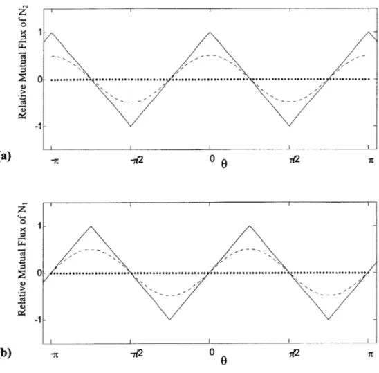
term stays constant. This point will be reemphasized after torque is derived. A normalized plot of mutual flux of A2 and A, with respect to drag angle are plotted in

0 0 A Cc 1 -1 I 0 -1 I I I -It 712 0 -0 i2 IC -n -n2 0

e

Figure 3: (a) The solid line plots the linear mutual flux relation of X2 with respect to drag angle 0. A well designed motor with additional slots and windings about winding N2 can achieve a cosinusoidal

mutual flux linkage indicated by the dotted wave. (b) Mutual flux of X1.

(a)

2.4

Flux Linkage Approximation

The triangular variation of mutual flux linkage with respect to 0 is a result of modeling the stator and rotor windings as a single winding discretely distributed as shown in Figure 1. A practical motor would have additional slots for windings to be distributed sinusoidally so that flux linkages would also be distributed in the same manner. This configuration avoids discontinuities at multiples of R/2 where mutual flux can transition abruptly from positive to negative slopes. The motor under study is evidently conFigured with sinusoidal windings because laboratory observation shows that its back emf is approximately sinusoidal. (One can be very keen and be able to observe harmonics in the back emf waveform that indicate saliency, but that is outside the scope of this derivation.) Figure 3a shows this ideal cosine mutual flux function for 2. It will be presently shown that a motor with sinusoidally varying flux linkages will produce constant torque when synchronously driven with sinusoidally varying current. The hysteresis motor under study is assumed to have this characteristic to ensure smooth operation.

Similarly, the mutual flux from N, can also be plotted, Figure 3b. Its ideal distribution looks sinusoidal because according to (28), N1 exhibits zero mutual flux

when drag angle 0 = 0 and increases with increasing 0 until zr/4. Figure 1 demonstrates that when 0 = 0, half of the rotor flux flowing through NI's cross section augments, while the other half of the rotor flux attenuates its flux. Once 0 = 7r/4, the rotor flux area aligns itself with Ni's windings all around the motor such that A, is maximized.

Examining 2's mutual flux expression in (27) and comparing it to Figure 3a, the

0 dependent term in (27) is equivalent to a cosine function. Similarly, the 0 dependent term in (28) resembles a sine function:

I - 4 cos 20 (30)

H

Applying these approximations to (27), (28), and (29) the flux linkage expressions become:

'2 = N2 "LR;T (N2 2 + Ni, cos 20) (32)

2g

N=

N " (Ni, + N.i, sin 20) (33)

2g

;,.r=N,. 2g~c(N., + N2J2 cos 29 + Ni sin 2 (34)

2.5

Motor Torque Expression

Having found flux linkages for all the windings in the motor, its coenergy can be found using Woodson and Melcher's formula (20). For simplification, let:

L -= (35)

2g

'2 il i, W'= fZ2di + fAdi + fA,di'

0 0 0

W'= N2LoijN2i2 + Nr,, cos 20) + NLOiIKN l( + Nrir sin 20

+ NrLoir r j + N2i2 cos 20 + Nii, sin 20) (36)

Differentiating (36) with respect to 0 according to (21) gives torque:

T = 4NirNiLO cos20-4NrirN2i2Lo sin 20 T = 2Ni, " (Ni1 cos 20 -N i22 sin 20)

g (37)

Notice that torque depends entirely on mutual flux. The self flux terms drop out when W' is differentiated, because they do not depend on 0. A practical motor would have the same number of turns for each of its windings so that N1 = N2 = N. Therefore, (37) can

be expressed as:

T = 2NrNs " LOR;T i, (I cos 20-i 2 sin 20)

T = 2Mi, (i1 cos 20- i2 sin 20) (38)

where M is considered the mutual inductance of the motor:

M = NrNs ,LRir

g (39)

Throughout this derivation, a snapshot in time of the rotor and stator relationship is made to arrive at the flux linkages in terms of 0. The torque expression (38) shows only an instance in time when currents ir, il, i2, and drag angle 0 have definite values. It

assumes a static frame of reference whereby the observer is rotating along at the same mechanical rate as the rotor, so that 0 seems constant.

To understand the dynamics of the motor, the frame of reference needs to be changed. The observer will now look at the motor from a static vantage point, the stator. In other words, the observer is looking at the rotor spinning with time. Since the observer does not move with the rotor, the rotor is going to exhibit an increase in angle. The term ''rotor angle" is now introduced as:

r = Qt -0 (40)

where Q is the mechanical speed of the motor with respect to time. It not only expresses the speed of the rotor, but can also describe the speed of the stator magnetic field at synchronous speed. That said, 0 is, as stated before, the drag angle between the rotor and stator's magnetic field. The negative sign in front of 0 is attributed by the fact that rotor phase lags behind the stator magnetic phase. In other words, 0= 12t + y.

Imposing a time dependence on the stator currents results in the following expressions:

i1 = i, sin cot (41)

i2 = is cos ait (42)

where o, is the electrical motor rate. Since the rotor acts like a permanent magnet, it does not have time dependence, so its current is expressed as a constant:

ir = Ir (43)

These currents produce a torque of

T = 2MIIs(sin cot cos2; - cos wt sin2y) (44)

Using the trigonometric identity:

(44) becomes:

T = 2MIIrs sin(cot - 2y)

T = 2MI,1, sin(cost - 2Qt + 20). ₍₄₆₎

In a four-pole motor, the mechanical motor speed Q is half the rate of the electrical speed:

2

(47)

so that torque becomes independent of time and depends on current amplitudes and drag angle:

T = 2MIrs sin(20).

The next section reaffirms this point through a different approach.

CHAPTER 3

Motor Dynamic Behavior

Having found a time dependent motor torque expression (46), it is possible to analyze the dynamic behavior of the motor by now incorporating wheel inertia and friction into the analysis. The following section relates these factors to the drag angle 9.

The dynamic behavior of the motor can be expressed as a second order ordinary differential equation:

d2_{9 dO}

J 2+ B- + 2MIrs sin(co t - 27)=T) (49)

dt2 _dt

where J is the wheel's moment of inertia, which includes the rotor and flywheel assembly. B is the drag coefficient of bearing friction and wind drag on all moving surfaces. TL(t), the load torque, is considered to be the driving factor because it may be an external disturbance to the motor that causes transients in rotor angle, y. The left side of (49) represents an oscillatory second order system with damping provided by B. A change in TL(t) excites the system and causes y to oscillate.

To find the operating drag angle 9 under the ideal synchronous operation, where no external disturbances are applied, TL(t) is set to zero and by substituting (40) for 7:

0 = J d - 0)+ B d (Ot - 0)+ 2 MIjI sin (cot - 2(Qt - 0))

dt dt

0 = Bi + 2M~rIs sin ((CoS - 2Q)t + 20)

BQ = -2 MI. JS sin ((Cos - 2Q)t + 20) ₍₅₀₎

This expression makes intuitive sense because once the motor is at synchronous speed, the wheel's inertia J does not affect the time rate of change in rotor angle. Since B and Q are constants, the right hand side of this equation is constant and in order for (50) to be true, the time varying term inside the sine expression must be zero so that:

Q = (51)

2

which reaffirms that the motor's mechanical speed runs at half the electrical speed. Substituting this value back into (50) reveals that the torque produced by the motor in the absence of external disturbances is constant:

T = 2M.rIs sin 20 (52)

Rearranging (50), drag angle 0 can now be expressed as:

0= 1sin _, - B Q (

b ( d

I

2M ,J,

a

Figure 4: Graph of T = 2Mr,s sin 29 where points a, b, c, and d are possible values of 9, the operatin drag angle.

This makes intuitive sense because as friction, B, and drag are increased, the drag angle would also increase. If the amplitude of the drive currents is increased, thereby increasing the magnetic intensities of the rotor and stator, then the drag angle decreases. The only concern in (53) is the half factor. It can be generalized that the half factors represents the motor's number of pole pairs.

As pointed out earlier, the motor's mechanical speed Q is half that of the electrical excitation speed, o),. In general, the mechanical speed of the motor is:

a) =

P (54)

where p is the number of pole pairs. The motor under study has four poles, therefore two pole pairs. Thus, the drag angle can be generalized as:

=-s I sin(55)

P PMI,.it

Equation (53) implies that:

A

b c d

1 (56) 2M1,.I

and that there are four possible solutions to 0 for one mechanical cycle around the motor as depicted in Figure 4. These possible angles will be examined for stability in the next section when external disturbances are added to the motor to induce hunting.

3.1

Second Order Effects on Drag Angle 0

While the motor spins with a nominal drag angle of 0, there exist sudden disturbances from inconsistent bearing friction and vibrations from outside the motor that can offset this angle by small amounts 0'(t). The sudden increase in friction can cause 0 to widen momentarily and the motor will react by outputting more torque than nominal. This in turn causes the rotor to overshoot its operating equilibrium point 0 and hunt about until damping from hysteresis braking or viscous drag settles it back to a steady 0.

During a hunting transient, the rotor angle can be represented as:

Y = ft - 0 - '0t0 (57)

Substituting this back into the dynamic motor equation (49):

d2d (58)

J' (t -0 - 0'(t ))+ B -(Qt - 0 - '(t))+ 2MIr s sin[w>,t - 2(Qt - 0 -

o'(t))]

dt dt

The first and second terms are easily evaluated by differentiating the rotor angle expression, but the nonlinear sine term needs to be approximated using Taylor expansion:

1 (9

f(x) = f(a)+(x - a)f'(a)+-(x - a)2 _{f"(a)+... (59)}

In this expression, a is the center point about which the approximation is taken. For the motor, a is equal to 20. The variable x can be considered the angle inside the sine

function such that:

x= O)St - 2(Qt - 0 - 01'(t

))

x =20 + 20(t)

which shows the equilibrium drag angle, 20, and its first order variation 20'(t). The sine expression approximates to:

2MIIs sin 2(0 + 0'(t ))= 2M1,1,[sin(20) + (20 + 20'(t) - 20)cos 20]

2M,Js sin 2(0 + 0'(t))= 2MI, (sin 20 + 20'(t) cos 20) (61)

Recalling that BO = -2MrIssin20, (58) simplifies to a second order differential equation:

J d 0'(t) + B -0'(t) + BQ + 2MIJ, sin 20+20'(t)(2MrI, cos 20) = TL (t)

d7 dt

d2 B d 2(2MIIs cos20)

7 1',(t) +--0'(t) + ' 0' W' = TL (62

dt 2 ' Jdt J (62)

For convenience, let

K = 2(2MIIs cos 20) (63)

The technique for solving (62) by calculating the homogenous and then guessing the particular solution can be applied. Notice that K is analogous to the spring constant in a mass/spring/dashpot system. In this analogy, 0 is the resting length of the spring, while

O'(t) is a displacement from this length that causes the spring to pull back. The spring

constant looks nonlinear with respect toQ, but bear in mind that it is assumed to be very small. Thus, K can be treated as a constant.

The homogenous solution is found by solving the characteristic equation. Using the quadratic formula, two natural frequencies are found, s1 and s2:

2B K s2 + s + 0 (64) J J B (B 2 _K S + -- (65) 2J 2J J B B K (66) s2 - D6 2J 2J J

The homogenous solution is of the form:

0'h ( =Ceslt + C2e S2 (67)

By defining the disturbance torque to be a small step function:

TL( 0) = 0 (68)

TL(t > 0) = T (69)

initial conditions can be established so that C, and C2 can be calculated. Keeping in mind

that the general solution becomes the particular solution some time after the step function is applied, it is reasonable to guess that:

TJ (70)

K

by checking with equation (62). The general solution is now:

0(t)= -+Cet +C2eS21

K (71)

Using the following initial conditions:

0'(t = 0)= 0 (72)

d (73)

-'(t = 0) = 0 dt

TJ (74) 0 =-Tj+C1 +C2 (4 K 0 = CIs1 + C2s2 (75) After manipulation: TJ s2 C, = 276) K s -s 2 TJ s C2 =- (77) K s2 -s1

so that the total solution for the hunting rotor angle is:

9'(t) = -jl+ S₂ es" + s' e 2t' (78)

K s1 - s2 s2 -s1

As defined previously, s, and s2 as well as K are all dependent on the operating drag angle . Figure 4 demonstrates that there are four possibilities for , so it is necessary to test each one to assure that the solution converges. Since s, and s2

determines how fast the exponentials grow or decay, they are the first factors to be examined.

B

Looking at sj from (65), it is reasonable to consider that when K is zero, the

-2J

term outside the radical is equivalent to the - term inside the radical, so that sj is

2J

zero. If K were negative, then the term inside the radical would be positive, causing s, to be purely real and positive. This means that the second term of (78) would diverge and

the system would be unstable. However, when K is positive and that:

- > -- (79)

the terms inside the radical would be negative and s1 and s2 would be complex. The

sinusoidal hunting behavior of the hysteresis motor, as measured in the lab, suggests that

s, and S2 are indeed complex.

Since K is proportional to cos20, (63), it will be negative when:

z 37r (80)

4 4

and positive when:

(81) 10 <

-4

Therefore, in Figure 4, the operating angle at point b and d are invalid. The angle at points a and c assure stable operation.

For convenience, let's assign s and S2's real part as a and their imaginary part as

(Oh: B a - (82) 2J B2 K Ch = 1 - (83)

Substituting into (78) resuls in:

TJ

(

(a

9'(t) = - ee (84)

K 2icoh 2_icoh

After careful manipulation of Eulor's formula,

TJ~ (

>1(85)

V'()= - e- ' Cos OV t + -sin coht( 5

K _coh

3.2

Comparing Analytical Expression with Lab Results

This analytical expression is verified by comparing it to measured lab results. Measurements were taken by running the motor up to speed at 8Vrms and then applying a 10% step in drive magnitude to disturb it. The motor's measured hunting transient resembles a decaying sinusoid with a damping coefficient of a = -1/4.6 and a natural frequency of Oh = 4.3Hz. Plugging these values into (85) and plotting with Matlab results

in the solid line chart in Figure 5a. For comparison, the dotted chart in Figure 5a is the Simulink simulation output of the hunting rotor angle rate. Figure 5b shows the actual lab measurement of the hunting current transient. The following section will apply lab measurements to the analytically developed expressions to arrive at a transfer function for the motor dynamics.

~

tI

with Simulink Output for 7.SVrms Run

*j~~ ~ T -Fj~~

I N

0 2 4 6 8 10

time (sec)

12 14 16 18 20

Figure 5a: Plot of 0 '(t) transient response to an arbitrary step disturbance (solid line). The Simulink model transient response (dotted line) affms that the analytical derivation agrees with the empirical development.

Lab Measurement of Hunting Transient Step Response

0 2 4 6 8 10

time (sec)

12 14 16 18 20

Figure 5b: Plot of the transient current response to a step in drive voltage from 7.5 Vrms to 8.OVrms. Since the current indicates directly the drag angle, comparison of Figure 5a to 5b is valid as long as only the AC component of the sinusoid is considered.

cn 1512 1511 1510 1509 1508 1507 1506 1505 1504 0.03 0.02 0.01 UK E C Q. 0 -0.01 -0.02 -0.03

'V

VV

VV

V) II

CHAPTER 4

Bridging Analysis with Empirical Measurements

When the motor is driven with a 7.5Vrms voltage, its measured hunting transient resembles a decaying sinusoid with a damping coefficient of -1/4.6 and a natural frequency of 4.3Hz. The above analytical examination of the motor defined the friction coefficient B and motor spring constant K based on physical motor parameters and drive currents. It is now possible to relate these expressions to measured data to accurately predict how the motor behaves under disturbances.

The expression for the damping coefficient c is given by (82) and measured to be:

1 B

- a=- (86)

4.6 2J

Given that the wheel's moment of inertia J is 112 dyne*cm*sec^2 / rad, the drag coefficient is:

1

B=2J =51.7dyne*cm*sec (87)

4.6

This result is very close to the empirical value of 54 for the Simulink model.

The spring constant K resides inside the expression for the hunting frequency (Oh (83). Since hunting resembles a sinusoid, wh is imaginary:

B2K

(t-h = (88)

(2J J

so that K is solved as:

2 2K - oh a _ J K = J{Ojh 2 +a2) K =112 (2; * 4.3)2 +(41 K = 93.57 x IO3 _{dyne * cm *rad} (89)

Plugging these values back into the hunting angle differential equation (62) and applying

the Laplace transform gives a transfer function for the hunting angle with respect to a

disturbance torque:

2 51.7 93.57 x 103 TL(S)

112 112 O'(s)

H(s) = ='(s) _ 1

TL(s) + .462s + 836 (90)

Note that this transfer function can change with starting voltage and drive current.

Lab measurements indicate that an increase in operating voltage results in a higher spring

constant that speeds up the hunting frequency, Oh. For example, when the motor runs at

8Vrms and it is measured that (O = 4.6Hz and a = 1/4.7, then the transfer function would

be:

H

TL(s) S2 _+.425s+835

(91)

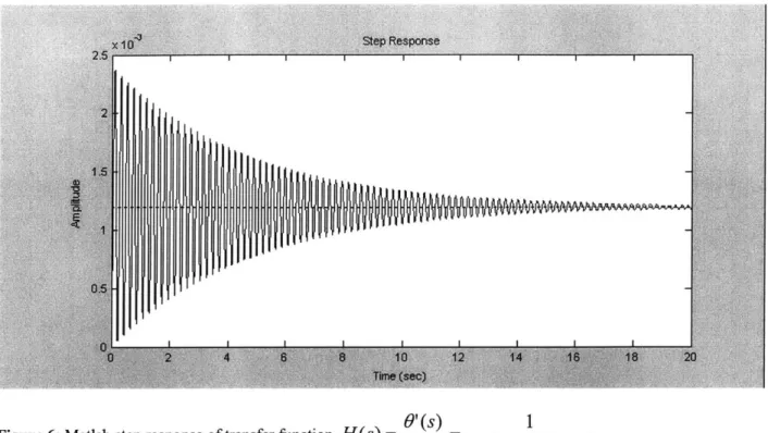
For verification purpose, this transfer is charted in Figure 6 using Matlab's Step

command. The result compares favorably with the lab measurement of Figure 5b and the

9'(s) 1 Figure 6: Matlab step response of transfer function H(s)= =

CHAPTER

5

Scheme for Damping the Hunting

The fundamental problem with the synchronous motor under study is that it is used to drive an inertial load rather than a viscous load. With an inertial load, such as the flywheel in the gyroscope, the motor does not exhibit much torque once it stops accelerating when it reaches synchronous speed. This means that it is susceptible to bearing noise and external vibrations, because the relative output torque to noise ratio is low. If the motor were driving a heavy viscous load where it must maintain a high output torque even at terminal velocity, any small variation in load torque from bearing noise is relatively small and unobservable.

One can make an analogy between this bearing noise with crossover distortion in a class-AB amplifier. If a deadzone exists in the amplifier, one can definitely hear the distortion at low volume levels, because the deadzone takes up a relatively significant amount of time per cycle compared to the signal. However, when the amplifier is delivering high voltage levels, the deadzone takes up a relatively small amount of time compared to the signal. Therefore, the signal masks the distortion.

Looking back at the torque vs drag angle chart in Figure 4, it is clear that since the motor drives a flywheel, it operates with a torque and drag angle very close to the origin.

considered hunting. There are two degrees of freedom that can be exploited to control this hunting. The magnitude of the torque curve can be stretched up and down (AM modulation), or the phase of the torque curve can be shifted right and left to maintain a

steady drag angle (FM modulation).

5.1

FM Modulation Chosen Over AM

Because the motor is driving a gyro wheel, it is desirable that it maintains a constant rotor velocity. Fluctuation in wheel velocity, hunting, is indicative of drag angle

0 deviations. Therefore, suppressing hunting involves controlling drag angle 0.

The mutual flux linkage between the rotor and the stator give direct indication of drag angle changes in the form of back emf, If driven by a constant voltage source, the motor current changes with back emf. One would immediately think that hunting is suppressible by modulating the motor current -[. By reexamining the torque expression repeated here:

T = 2M,1, sin 20 (92)

it is evident that since drag angle, 0, is so small, changes in torque T is negligibly small when modulating I. Looking at the torque angle curve of Figure 4, this implementation is considered Amplitude Modulation because it varies the magnitude of the torque curve. Because the drag angle is so small, changing the magnitude does not move the drag angle by much, rendering AM modulation ineffective.

A more effective way of controlling drag angle 0 is by modulating the stator phase itself co. Recalling the elaborated torque expression:

T = 2MIIs sin(cot - 2y)

T = 2MI1, sin(wct - 2Qt + 20). ₍₉₃₎

it is clear that cs superimposes directly on the drag angle within the sine expression. Direct control of 0 looks promising and it is the chosen scheme that is used to control.

Conceptually, when the rotor swings ahead of its operating drag angle, the back emf increases as though the motor is about to generate power. This causes current amplitude going into to motor terminals to decrease. Conversely, when the rotor lags behind the nominal drag angle, the motor will demand more current.

5.2

Hunting Suppression Implementation

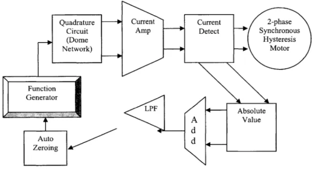
The compensation scheme monitors the current amplitude changes as an indication of drag angle. It increases the drive frequency, ws, when current decreases and vice versa when detected current increases. The transfer function of drag angle to input torque:

H(s)

TL S 2

+.425s + 835 (94)

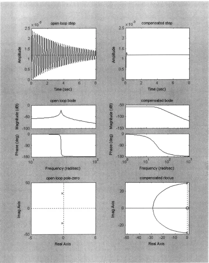
is directly proportional to input current is. Its characteristic poles look like a complex conjugate pair that resides very close to the

jo

Compensating this complex pole pair is difficult. Ideally, one would want to put a zero at the origin to cancel out one of the poles in closed loop. By virtue of FM modulation, this scheme is achievable. An Agilent function generator, model 33220A, is used in the compensation loop to drive the motor at os = 480Hz and modulate os by the