Averting Catastrophes: The Strange Economics of Scylla and Charybdis

Economics of Scylla and Charybdis

The MIT Faculty has made this article openly available.

Please share

how this access benefits you. Your story matters.

Citation

Martin, Ian W. R. and Pindyck, Robert S. “Averting Catastrophes: The

Strange Economics of Scylla and Charybdis.” American Economic

Review 105, no. 10 (October 2015): 2947–2985. © 2015 American

Economic Association

As Published

http://dx.doi.org/10.1257/aer.20140806

Publisher

American Economic Association

Version

Final published version

Citable link

http://hdl.handle.net/1721.1/109147

Terms of Use

Article is made available in accordance with the publisher's

policy and may be subject to US copyright law. Please refer to the

publisher's site for terms of use.

2947

Averting Catastrophes:

The Strange Economics of Scylla and Charybdis

By Ian W. R. Martin and Robert S. Pindyck*

Faced with numerous potential catastrophes—nuclear and bioter-rorism, mega-viruses, climate change, and others—which should

society attempt to avert? A policy to avert one catastrophe con-sidered in isolation might be evaluated in cost-benefit terms. But because society faces multiple catastrophes, simple cost-benefit

analysis fails: even if the benefit of averting each one exceeds the cost, we should not necessarily avert them all. We explore the policy

interdependence of catastrophic events, and develop a rule for

deter-mining which catastrophes should be averted and which should not.

(JEL D61, Q51, Q54)

“‘Is there no way,’ said I, ‘of escaping Charybdis, and at the same time

keeping Scylla off when she is trying to harm my men?’

“‘You dare-devil,’ replied the goddess, ‘you are always wanting to fight

somebody or something; you will not let yourself be beaten even by the immortals.’”

—Homer, Odyssey1

Like any good sailor, Odysseus sought to avoid every potential catastrophe that might harm him and his crew. But, as the goddess Circe made clear, although he could avoid the six-headed sea monster Scylla or the “sucking whirlpool” of Charybdis, he could not avoid both. Circe explained that the greatest expected loss would come from an encounter with Charybdis, which should therefore be avoided, even at the cost of an encounter with Scylla.

We modern mortals likewise face myriad potential catastrophes, some more daunting than those faced by Odysseus. Nuclear or bioterrorism, an uncontrolled viral epidemic on the scale of the 1918 Spanish flu, or a climate change catastrophe

1 _{Odyssey, Book XII, translated by Samuel Butler (1900).}

* Martin: London School of Economics, Houghton Street, London WC2A 2AE, UK (e-mail: i.w.martin@ lse.ac.uk); Pindyck: Sloan School of Management, Massachusetts Institute of Technology, 100 Main Street, Cambridge, MA 02139 (e-mail: rpindyck@mit.edu). Our thanks to Thomas Albert, Robert Barro, Simon Dietz, Christian Gollier, Derek Lemoine, Bob Litterman, Deborah Lucas, Antony Millner, Gita Rao, Edward Schlee, V. Kerry Smith, Nicholas Stern, Martin Weitzman, three anonymous referees, and seminar participants at LSE, Oxford, the University of Amsterdam, Tel-Aviv University, Universidad de Chile, Harvard, MIT, the University of Arizona, Arizona State University, and the Toulouse School of Economics for helpful comments and suggestions. Ian Martin is supported by ERC Starting Grant 639744. Both authors declare that they have no relevant or material financial interests that relate to the research described in this paper.

† _{Go to http://dx.doi.org/10.1257/aer.20140806 to visit the article page for additional materials and author} disclosure statement(s).

are examples. Naturally, we would like to avoid all such catastrophes. But even if it were feasible, is that goal advisable? Should we instead avoid some catastrophes and accept the inevitability of others? If so, which ones should we avoid? Unlike Odysseus, we cannot turn to the gods for advice. We must turn instead to economics, the truly dismal science.

Those readers hoping that economics will provide simple advice, such as “avert a catastrophe if the benefits of doing so exceed the cost,” will be disappointed. We will see that deciding which catastrophes to avert is a much more difficult problem than it might first appear, and a simple cost-benefit rule doesn’t work. Suppose, for example, that society faces five major potential catastrophes. If the benefit of avert-ing each one exceeds the cost, straightforward cost-benefit analysis would say we should avert all five.2 _{We show, however, that it may be optimal to avert only (say)} three of the five, and not necessarily the three with the highest benefit_{/cost ratios.} This result might at first seem “strange” (hence the title of the paper), but we will see that it follows from basic economic principles.

Our results highlight a fundamental flaw in the way economists usually approach potential catastrophes. Consider the possibility of a climate change catastrophe—a climate outcome so severe in terms of higher temperatures and rising sea levels that it would sharply reduce economic output and consumption _{(broadly understood). A} number of studies have tried to evaluate greenhouse gas (GHG) abatement policies by combining GHG abatement cost estimates with estimates of the expected bene-fits to society (in terms of reduced future damages) from avoiding or reducing the likelihood of a bad outcome.3 _{To our knowledge, however, all such studies look at} climate change in isolation. We show that this is misleading.

A climate catastrophe is only one of a number of catastrophes that might occur and cause major damage on a global scale. Other catastrophic events may be as likely or more likely to occur, could occur much sooner, and could have an even worse impact on economic output and even mortality. One might estimate the ben-efits to society from averting each of these other catastrophes, again taking each in isolation, and then, given estimates of the cost of averting the event, come up with a policy recommendation. But applying cost-benefit analysis to each event in isolation can lead to a policy that is far from optimal.

Conventional cost-benefit analysis can be applied directly to “marginal” proj-ects, i.e., projects whose costs and benefits have no significant impact on the overall economy. But policies or projects to avert major catastrophes are not marginal; their costs and benefits can alter society’s aggregate consumption, and that is why they cannot be studied in isolation.

Like many other studies, we measure benefits in terms of willingness to pay (WTP), i.e., the maximum fraction of consumption society would be willing to 2 _{Although we will often talk of “averting” or “eliminating” catastrophes, our framework allows for the} possi-bility of only partially alleviating one or more catastrophes, as we show in Section IVA.

3 _{Most of these studies develop integrated assessment models (IAMs) and use them for policy evaluation. The} literature is vast, but Nordhaus (2008) and Stern (2007) are widely cited examples; other examples include the many studies that attempt to estimate the social cost of carbon (SCC). For a survey of SCC estimates based on three widely used IAMs, see Greenstone, Kopits, and Wolverton (2013) and Interagency Working Group on Social Cost of Carbon (2010). These studies, however, generally focus on “most likely” climate outcomes, not low-probability catastrophic outcomes. See Pindyck (2013a,b) for a critique and discussion. One of the earliest treatments of envi-ronmental catastrophes is Cropper (1976).

sacrifice, now and forever, to achieve an objective. We can then address the fol-lowing two questions: first, how will the WTP for averting Catastrophe A change once we take into account that other potential catastrophes B, C, D, etc., lurk in the background? We show that the WTP to eliminate A will go up.4 _{The reason is} that the other potential catastrophes reduce expected future consumption, thereby increasing expected future marginal utility and therefore also the benefit of averting catastrophe A. Likewise, each individual WTP _{(e.g., to avert just B) will be higher} the greater is the “background risk” from the other catastrophes. What about the WTP to avert all of the potential catastrophes? It will be less than the sum of the individual WTPs. The WTPs are not additive; society would probably be unwilling to spend 60 or 80 percent of gross domestic product _{(GDP) (and could not spend} 110 percent of GDP) to avert all of these catastrophes.

WTP relates to the demand side of policy: it is society’s reservation price—the

most it would sacrifice—to achieve some goal. In our case, it measures the benefit of averting a catastrophe. It does not tell us whether averting the catastrophe makes economic sense. For that we also need to know the cost. There are various ways to characterize such a cost: a fixed dollar amount, a time-varying stream of expen-ditures, etc. In order to make comparisons with the WTP measure of benefits, we express cost as a permanent tax on consumption at rate _{τ , the revenues from which} would just suffice to pay for whatever is required to avert the catastrophe.

Now suppose we know, for each major type of catastrophe, the correspond-ing costs and benefits. More precisely, imagine we are given a list ( τ 1 , w 1 ) , ( τ 2 , w 2 ) , … , ( τ N , w N ) of costs ( τ i ) and WTPs ( w i ) associated with projects to

eliminate N different potential catastrophes. That brings us to our second question: which of the N projects should we implement? If _{w i > τ i for all i , should we} elim-inate all N potential catastrophes? Not necessarily. We show how to decide which projects to choose to maximize social welfare.

When the projects are very small relative to the economy, and if there are not too many of them, the conventional cost-benefit intuition prevails: if the projects are not mutually exclusive, we should implement any project whose benefit w _i exceeds its cost _{τ i . This intuition might apply, for example, for the construction of a dam to avert} flooding in some area. Things are more interesting when projects are large relative to the economy, as might be the case for the global catastrophes mentioned above, or if they are small but large in number (so their aggregate influence is large). Large projects change total consumption and marginal utility, causing the usual intuition to break down: there is an essential interdependence among the projects that must be taken into account when formulating policy.

We are not the first to note the interdependence of large projects; early expositions of this point include Dasgupta, Sen, and Marglin _{(1972) and Little and Mirrlees} (1974). (More recently, Dietz and Hepburn 2013 illustrate this point in the context of climate change policy._{) Nor are we the first to note the effects of background risk;} see, e.g., Gollier (2001) and Gollier and Pratt (1996). But to our knowledge this paper is the first to address the question of selecting among a set of large projects.

We show how this can be done, and we use several examples to illustrate some of the counterintuitive results that can arise.

For instance, one apparently sensible response to the nonmarginal nature of large catastrophes is to decide which is the most serious catastrophe, avert that, and then decide whether to avert other catastrophes. This approach is intuitive and plausi-ble—and wrong. We illustrate this in an example with three potential catastrophes. The first has a benefit _{w 1 much greater than the cost τ 1 , and the other two have} ben-efits greater than the costs, but not that much greater. Naïve reasoning suggests we should proceed sequentially: eliminate the first catastrophe and then decide whether to eliminate the other two, but we show that such reasoning is flawed. If only one of the three were to be eliminated, we should indeed choose the first; and we would do even better by eliminating all three. But we would do best of all by eliminating the second and third and not the first: the presence of the second and third catastrophes makes it suboptimal to eliminate the first.

In the next section we use two very simple examples to illustrate the general interdependence of large projects, and show why, if faced with two potential catastrophes, it might not be optimal to avert both, even if the benefit of averting each exceeds the cost. In Section II we introduce our framework of analysis by first focusing on the WTP to avert a single type of catastrophe _{(e.g., nuclear} ter-rorism) considered in isolation. We use a constant relative risk aversion (CRRA) utility function to measure the welfare accruing from a consumption stream, and we assume that the catastrophe arrives as a Poisson event with known mean arrival rate; thus catastrophes occur repeatedly and are homogeneous in time. Each time a catastrophe occurs, consumption is reduced by a random fraction.5 _These simpli-fying assumptions make our model tractable, because they imply that the WTP to avoid a given type of catastrophe is constant over time.

This tractability is critical when, in Section III, we allow for multiple types of catastrophes. Each type has its own mean arrival rate and impact distribution. We find the WTP to eliminate a single type of catastrophe and show how it depends on the existence of other types, and we also find the WTP to eliminate several types at once. We show that the presence of multiple catastrophes may make it less desirable to try to mitigate some catastrophes for which action would appear desirable, considered in isolation. Next, given information on the cost of eliminating (or reducing the likelihood of) each type of catastrophe, we show how to find the welfare-maximizing combination of projects that should be undertaken.

Section IV presents some extensions. First, we show that our framework allows for the partial alleviation of catastrophes, i.e., for policies that reduce the likelihood of catastrophes occurring rather than eliminating them completely. The paper’s central intuitions apply even if we can choose the amount by which we reduce the arrival rate of each catastrophe optimally. Second, our framework easily handles catastrophes that are directly related to one another: for example, averting nuclear terrorism might also help avert bioterrorism. Third, our results also apply to bonanzas, that is, to projects 5 _{Similar assumptions are made in the literature on generic consumption disasters. Examples include Backus,} Chernov, and Martin (2011); Barro and Jin (2011); and Pindyck and Wang (2013). Martin (2008) estimates the welfare cost of consumption uncertainty to be about 14 percent, most of which is attributable to higher cumulants (disaster risk) in the consumption process. Barro (2013) examines the WTP to avoid a climate change catastrophe with (unavoidable) generic catastrophes in the background.

such as blue-sky research that increase the probability of events that raise consump-tion (as opposed to decreasing the probability of events that lower consumption).

The contribution of this paper is largely theoretical: we provide a framework for analyzing different types of catastrophes and deciding which ones should be included as a target of government policy. Determining the actual likelihood of nuclear terrorism or a mega-virus, as well as the cost of reducing the likelihood, is no easy matter. Nonetheless, we want to show how our framework might be applied to real-world government policy formulation. To that end, we survey the (very lim-ited_{) literature for seven potential catastrophes, discuss how one could come up} with the relevant numbers, and then use our framework to determine which of these catastrophes should or should not be averted.

I. Two Simple Examples

Why is it that “large,” i.e., nonmarginal projects are inherently interdependent and cannot be evaluated in isolation? The following simple examples should help convey some of the basic intuition, and also clarify the connection between our work and the prior literature. The first example addresses a (static) decision to undertake a set of projects, and shows how the decision rule changes if the projects are large. The second example asks whether resources should be sacrificed today to avert one or two catastrophes that will otherwise occur in the future. It illustrates the effect of background risk, the interdependence of WTPs, and the connection to cost-benefit analysis.

Static Example: Suppose we are deciding whether to undertake two independent projects.6 _{To make the basic point in the simplest possible case, we assume that these} are yes_{/no projects, so that the resources expended on project i , e i , equals either 0} or x _i . We can approximate net welfare, W , using a second-order Taylor expansion: (1) W( e 1 , e 2 ) ≈ W(0, 0) +

∑

|

∑

∑

|

If both projects are “marginal,” i.e., the x _i are very small, then we can ignore the second-order term in _{(1), and the optimal decision is to set e i = x i} if ∂ W/∂  e _i  

|

e 1 = e 2 =0 > 0 and e i = 0 otherwise. In other words, the standard cost-benefit rule applies: undertake a project if doing so yields an increase in net welfare. But if the projects are not marginal, then we cannot ignore the second-order term in _{(1). Now the standard cost-benefit rule fails. Why? Because of the second} derivative terms, the value of project 1 depends on whether project 2 is also being carried out, and vice versa. Thus large projects cannot be evaluated independently of each other.7

6 _{A version of this example was suggested by an anonymous referee, whom we thank.}

7 _{This is essentially the idea behind Dasgupta, Sen, and Marglin (1972) and Little and Mirrlees (1974). Also,} note that this interdependence does not depend on the binary (i.e., e i = 0 or x i ) nature of the projects. As we show in

Two-Period Example: As a second example, suppose there are two potential catastrophes that, if not averted, will surely occur at a future time T . Each catastrophe will reduce consumption at time T by a fraction _{ϕ . Consumption today is C 0 = 1 ,} so consumption at T is C _T = 1 if both catastrophes are averted, C _T = 1 − ϕ if one is averted, and _{C T = (1 − ϕ)} 2 _{if neither is averted. Each catastrophe can be averted} by sacrificing a fraction τ of consumption today and at time T . We assume CRRA utility and ignore discounting, so welfare is

V _{= 1} _____

1 − η [ C 01 −η + C T1 −η] ,

and for simplicity let η = 2 . If neither catastrophe is averted, welfare is V 0 = −[1 + (1 − ϕ) −2 ] .

If we avert one of the two catastrophes by sacrificing a fraction of consumption

w_{1 , welfare is V 1 = − (1 − w 1 )} −1 _[1 _{+ (1 − ϕ)} −1_{] . The WTP is the fraction w 1} that equates V 0 to V 1 : (2) w 1 = 1 −

_[

]

The WTP to avert both catastrophes, _{w 1, 2 , equates V 0 to V 1, 2 = −2 (1 − w 1, 2 )} −1 _{, so} (3) w 1, 2 = 1 − __________{1 + (1 − ϕ)} 2 ₋₂ .

Finally, if there were only one catastrophe, the WTP to avert it would be (4) w1′ = 1 −

[ _________1 _{+ (1 − ϕ)} 2 −1 _] .

We can use equations _{(2), (3), and (4) to illustrate several points:}

(i) Background risk increases the WTP to avert a catastrophe. It is easy to see that w 1 > w 1′ , i.e., the WTP to avert Catastrophe 1 is increased by the pres-ence of Catastrophe 2. For example, if _{ϕ = 0.5 , w 1 = 0.40 , and w 1′ = 0.33 .} Catastrophe 2 reduces C _T , raising marginal utility at time T , and thereby rais-ing the value of avertrais-ing Catastrophe 1.8

(ii) WTPs don’t add. Specifically, w 1, 2 < w 1 + w 2 . For example, if ϕ = 0.5 ,

w1, ₂ = 0.60 < w 1 + w 2 = 0.80 . Sacrificing 40 percent of consumption 8 _{This result is related to the notion of “risk vulnerability” introduced by Gollier and Pratt (1996). They derive} conditions under which adding a zero-mean background risk to wealth will increase an agent’s risk aversion with respect to an additional risky prospect. The conditions are that the utility function exhibits absolute risk aversion that is both declining and convex in wealth, a natural assumption that holds for all hyperbolic absolute risk aversion (HARA) utility functions. Risk vulnerability includes the concept of “standard risk aversion” (Kimball 1993) as a special case. In our model, background risk is not zero-mean: background events reduce consumption in our base-line framework and increase consumption in the extension in Section IVC.

sharply increases the marginal utility loss from any further sacrifice of consumption.

(iii) Naïve cost-benefit analysis can be misleading. More specifically, we might not avert a catastrophe even if the benefit of averting it—considered in iso-lation—exceeds the cost. For example, suppose ϕ = 0.5 as before, so that

w_{1 = w 2 = 0.4 . If τ 1 = τ 2 = 0.35 , the benefit of averting each}

catastro-phe exceeds the cost. But we should not avert both. For if we avert nei-ther catastrophe, net welfare is _{V 0 = −5 ; if we avert one, net welfare is}

W 1 = −4.62 ; and if we avert both, net welfare is W 1,₂ = −4.73 . Averting both is better than averting neither, but we do best by averting exactly one. To understand this, note that if we avert one catastrophe, what matters is whether the additional benefit from averting the second exceeds the cost, i.e., whether ( w 1,₂ − w 1 )/(1 − w 1 ) > τ 2 . We should not avert #2 because ( w 1, 2 − w 1 )/(1 − w 1 ) = 0.33 < τ 2 = 0.35 .

These examples help connect our work to the earlier literature and illustrate why large projects are interdependent. We turn next to a fully dynamic model that includes uncertainty over the arrival and impact of multiple potential catastrophes, and that lets us derive a key result regarding the set of catastrophes that should be averted.

II. The Model with One Type of Catastrophe

We first consider a single type of catastrophe. It might be a climate change catastrophe, a mega-virus, or something else. What matters is that we assume for now that this particular type of catastrophe is the only thing society is concerned about. We want to determine society’s WTP to avoid this type of catastrophe, i.e., the maximum fraction of consumption, now and throughout the future, that society would sacrifice. Of course it might be the case that the revenue stream correspond-ing to this WTP is insufficient to eliminate the risk of the catastrophe occurrcorrespond-ing, in which case eliminating the risk is economically infeasible. Or, the cost of elim-inating the risk might be lower than the corresponding revenue stream, in which case the project would have a positive net social surplus. The WTP applies only to the demand side of government policy. Later, when we examine multiple types of catastrophes, we will also consider the supply _{(i.e., cost) side.}

To calculate a WTP, we must consider whether the type of catastrophe at issue can occur once and only once _{(if it occurs at all), or can occur repeatedly. For a climate} catastrophe, it might be reasonable to assume that it would occur only once—the global mean temperature, for example, might rise much more than expected, causing economic damage far greater than anticipated, and perhaps becoming worse over time as the temperature keeps rising.9 _{But for most potential catastrophes, such as a} mega-virus, nuclear terrorism, or nuclear war, it is more reasonable to assume that the catastrophe could occur multiple times. Throughout the paper we will assume 9 _{That is why some argue that the best way to avert a climate catastrophe is to invest now in geoengineering} technologies that could be used to reverse the temperature increases. See, e.g., Barrett (2008, 2009) and Kousky et al. (2009).

that multiple occurrences are indeed possible. However, in an online Appendix we examine the WTP to eliminate a catastrophe that can occur only once.

We will assume that without any catastrophe, real per-capital consumption will grow at a constant rate g , and we normalize so that at time t = 0 , C 0 = 1 . Let

c_{t denote log consumption. We define a catastrophe as an event that permanently}

reduces log consumption by a random amount ϕ (so that ϕ is roughly the fraction by which the level of consumption falls_{). Thus if the catastrophic event first occurs} at time t 1 , C t = e gt for t < t 1 and then falls to C t = e −ϕ+gt at t = t 1 . For now we impose no restrictions on the probability distribution for _{ϕ . We use a simple CRRA} utility function to measure welfare, and denote the index of relative risk aversion by η and rate of time preference by δ . Unless noted otherwise, in the rest of this paper we will assume that η > 1 , so utility is negative. This is consistent with both the finance and macroeconomics literatures, which put _{η in the range of 2–5 (or even} higher). Later we treat the special case of η = 1 , i.e., log utility.

We assume throughout this paper that the catastrophic event of interest occurs as a Poisson arrival with mean arrival rate λ , and that the impact of the n th arrival, ϕ _n , is independent and identically distributed across realizations n . Thus the process for consumption is

(5) c t = log  C t = gt −

∑

ϕ n ,

where Q_{(t) is a Poisson counting process with known mean arrival rate λ , so when the}

n th catastrophic event occurs, consumption is multiplied by the random variable e − ϕ n . We follow Martin _{(2013) by introducing the cumulant-generating function (CGF), κ t (θ) ≡ log E e} c t θ _{≡ log E  C}

tθ  .

As we will see, the CGF summarizes the effects of various types of risk in a conve-nient way. Since the process for consumption given in (5) is a Lévy process, we can simplify _{κ t (θ) = κ(θ)t , where κ(θ) means κ 1 (θ) . In other words, the t -period CGF} scales the 1-period CGF linearly in t . We show in the Appendix that the CGF is then10 (6) κ(θ) = gθ + λ

(

)

Given this consumption process, welfare is (7) E

∫

1 _{− η} e −δt  C t1 −η dt = 1 ______{1 − η}

∫

∞

e −δt_e κ(1−η)t _dt = 1 _____ _{1 − η} ________1 _{δ − κ(1 − η) ,}

10 _{We could allow for c}

t = g t − ∑ nN=1(t) ϕ n , where g t is any Lévy process, subject to the condition that ensures

finiteness of expected utility. (For the special case in (5), g t = gt for a constant g .) This only requires that the term gθ in the CGFs is replaced by g(θ) , where g(θ) is the CGF of g 1 , so if there are Brownian shocks with volatility σ , and jumps with arrival rate ω and stochastic impact J , then g(θ) = μθ + _{_}1

2 σ 2   θ 2 + ω ( E e θJ − 1) . This lets us handle Brownian shocks and unavoidable catastrophes without modifying the framework. Since the generalization has no effect on any of our qualitative results, we stick to the simpler formulation.

where _{κ(1 − η) is the CGF of equation (6) with θ = 1 − η . Note that equation (7) is} quite general and applies to any distribution for the impact ϕ . But note also that wel-fare is finite only if the integrals converge, and for this we need _{δ − κ(1 − η) > 0} (Martin 2013).

Eliminating the catastrophe is equivalent to setting _{λ = 0 in equation (6). We} denote the CGF in this case by κ (1) (θ) . (This notation will prove convenient later when we allow for several types of catastrophes._{) So if we sacrifice a fraction w of} consumption to avoid the catastrophe, welfare is

(8) (________ 1 − w) 1−η

1 − η ____________ _{δ − κ} (1)1 _{(1 − η)}   .

The WTP to eliminate the event (i.e., set λ = 0 ) is the value of w that equates (7) and _(8): 1 ____ 1 _{− η} ________1 δ − κ(1 − η) = (1 − w) 1−η ________ 1 _{− η} ___________{δ − κ} (1)1 _{(1 − η)} .

Should society avoid this catastrophe? This is easy to answer because with only one type of catastrophe to worry about, we can apply standard cost-benefit analysis. The benefit is w , and the cost is the permanent tax on consumption, _{τ , needed to} generate the revenue to eliminate the risk. We should avoid the catastrophe as long as w _{> τ . As we will see shortly, when there are multiple potential catastrophes} the benefits from eliminating each are interdependent, causing this simple logic to break down.11

III. Optimal Policy with Multiple Catastrophes

We now allow for multiple types of catastrophes, show how to find the WTP to avert each type, and examine the interrelationship among the WTPs. We can then address the issue of choosing which catastrophes to avert. We aim to answer the following question: given a list of costs and benefits of eliminating different types of catastrophes, which ones should we eliminate? The punch line will be given by Result 2 below: there is a fundamental sense in which benefits add but costs

multi-ply. This will imply that there may be a substantial penalty associated with imple-menting several projects. As a result, it may be optimal not to avert catastrophes whose elimination seems justified in naïve cost-benefit terms.

11 _{A referee suggested that we could have alternatively expressed benefits in terms of the growth rate of} con-sumption, rather than as a percentage of its level. Then WTP would be the maximum reduction in the growth rate society would be willing to sacrifice to avert a catastrophe. Expressing benefits this way is certainly reasonable. If the costs of averting catastrophes are likewise modeled as required reductions in the growth rate (which we think is much less reasonable), our dynamic model could be written in a static form. Modeling benefits and costs in terms of levels is the conventional approach, which we have chosen to maintain.

As before, we assume that a catastrophic event causes a drop in consumption. We also assume that these events occur independently of each other. So log consump-tion is (9) c t = log  C t = gt −

∑

∑

∑

where Q _i (t) is a Poisson counting process with mean arrival rate λ _i , and the CGF is (10) κ(θ) = gθ + λ 1

(

)

+ λ 2

(

)

(

)

Here we write ϕ _i for a representative of any of the ϕ _i,_n (since catastrophic impacts are all independent and identically distributed within a catastrophe type_{). If no} catastrophes are eliminated, welfare is again given by equation (7). In the absence of catastrophe type i , welfare is

1 ____

1 − η ___________{δ − κ} (i)1 _{(1 − η)} ,

where the i superscript indicates that λ _i has been set to zero. Thus willingness to pay to eliminate catastrophe i satisfies

(1 − w i ) 1−η _________ 1 − η ___________{δ − κ} (i)1 _{(1 − η)} = 1 _____1 − η ________1 δ − κ(1 − η) , and hence w i = 1 − ₍ δ − κ( 1 − η) __________ δ − κ (i) _{(1 − η) )} 1 ____ η−1 .

Similarly, the WTP to eliminate some arbitrary subset S of the catastrophes, which we will write as w _S , is given by

(11) (1 − w S ) 1−η = δ − κ

(S)

(1 − η) __________ _{δ − κ(1 − η) .}

(The superscript S on the CGF indicates that λ i is set to zero for all i ∈ S .) The next

result shows how w _S , the WTP for eliminating the subset of catastrophes, can be connected to the WTPs for each of the individual catastrophes in the subset.

RESULT 1: The WTP to avert a subset, S , of the catastrophes is linked to the WTPs

to avert each individual catastrophe in the subset by the expression

(12) (1 − w S ) 1−η − 1 =

∑

i∈S   [ (1 − w i )

PROOF:

The result follows from a relationship between κ (S) (θ) and the individual κ (i) _{(θ) . Note that κ} (i) _{(θ) = κ(θ) − λ}

i  0

(

)

∑ i  ∈S   λ i

(

)

(

κ (S) _.

₎

∑

_∑

(

)

where | S | denotes the number of catastrophes in the subset S , and hence

∑

i∈S δ − κ (i)

(1 − η)

__________ _{δ − κ(1 − η) =} (| S | − 1)(δ − κ(1 − η)) + (δ − κ ___________________________(S) (1 − η)) _{. δ − κ(1 − η)} Using _{(11), we have the result. ∎}

If, say, there are N _{= 2 types of catastrophes, then Result 1 implies that} (13) 1 _{+ (1 − w 1, 2 )} 1−η _{= (1 − w}

1 ) 1−η + (1 − w 2 ) 1−η  .

Thus we can express the WTP to eliminate both types of catastrophes, _{w 1, 2 , in terms} of w 1 and w 2 . But note that these WTPs do not add: since the function (1 − x) 1−η is convex, equation _{(13) implies that w 1, 2 < w 1 + w 2 , by Jensen’s inequality.}

By the same reasoning, it can be shown that w 1,_{2, … , N} < ∑ iN=1 w i . Likewise, if we

divide the N catastrophes into two groups, 1 through M and M _{+ 1 through N , then}

w1, _{2, … , N} < w 1,_{2, … , M} + w M+1, … , N . The WTP to eliminate all N catastrophes is less than the sum of the WTPs for each of the individual catastrophes, and less than the sum of the WTPs to eliminate any two groups of catastrophes.

A. Which Catastrophes to Avert?

The WTP, w _i , measures the benefit of averting Catastrophe i as the maximum fraction of consumption society would sacrifice to achieve this result. We measure the corresponding cost as the actual fraction of consumption that would have to be sacrificed, via a permanent consumption tax _{τ i , to generate the revenue needed to} avert the catastrophe. Thus we could avert all the catastrophes in some set S at the cost of multiplying consumption by _{∏ i  ∈S    (1 − τ i ) forever.}12, 13

12 _{This multiplicative cost assumption implies that it is cheaper in absolute terms to avert a given catastrophe if} the economy is small than if it is large. We think this is the natural formulation, because we also model the impact of catastrophes as multiplicative (and thus additive in logs, as in (9)), but we could alternatively have assumed that consumption was multiplied by 1 − ∑ i  ∈S   τ i . When costs are small relative to the aggregate economy we have

∏ i  ∈S    (1 − τ i ) ≈ 1 − ∑ i  ∈S   τ i , so the two assumptions are essentially identical. When costs are not small, our

multiplicative cost assumption is conservative, because it implies a smaller cost of averting groups of catastrophes than the alternative additive assumption would. But even with our multiplicative formulation, it will often not be optimal to avert catastrophes that, considered in isolation, appear to pass a cost-benefit hurdle.

13 _{As a referee pointed out, if the model is reformulated so that both benefits and costs affect the growth rate} rather than level of consumption, then the problem becomes separable and the standard cost-benefit rule applies. With respect to costs, we would then have consumption multiplied by a factor exp  ₍− ∑i  ∈S   τ i  t) . We have chosen

Thus, if we eliminate some subset S of the catastrophes, welfare _{(net of taxes) is} (14) _{__________________}∏ i  _∈S     (1 − τ i ) 1−η (1 − η)(δ − κ (S) _{(1 − η))} = ∏ i∈S   _{(1 − τ i )} 1_−η _________________________ (1 − η)(δ − κ(1 − η))(1 − w S ) 1−η ,

where the equality follows from _{(11). Our goal is to pick the set of catastrophes to} be eliminated to maximize this expression. To do so, it will be convenient to define (15) K i = (1 − τ i ) 1−η − 1 and Bi = (1 − w i ) 1−η − 1 .

Here K _i is the percentage loss of utility that results when consumption is reduced by τ i percent, and likewise for B i .

These utility-based definitions of costs and benefits are positive and increasing in _{τ i and w i , respectively, and K i > B i if and only if τ i > w i . For small τ i , we} have the linearization K _i ≈ (η − 1) τ _i ; and for small w _i , we have B _i ≈ (η − 1) w _i . The utility-based measures have the nice property that the _{B i s across catastrophes} are additive (by Result 1) and the K _i s are multiplicative. That is, the benefit from eliminating, say, three catastrophes is _{B 1, 2, 3 = B 1 + B 2 + B 3 , and the cost is}

K1, _2, 3 = (1 + K 1 )(1 + K 2 )(1 + K 3 ) − 1 . This allows us to state our main result in a simple form.

RESULT 2 _{(Benefits Add, Costs Multiply): It is optimal to choose the subset, S , of}

catastrophes to be eliminated to solve the problem

(16) max S⊆{1, … , N }   _{V =} 1 +

∑

(

)

where if no catastrophes are eliminated (i.e., if S is the empty set) then the objective function in _{(16) is taken to equal 1.}

PROOF:

If we choose some subset S then, using Result 1 to rewrite the denominator of expression _{(14) in terms of the individual WTPs, w i , expected utility equals}

______________________________________∏ i  ∈S   (1 − τ i ) 1−η (1 − η)

(

)

₍

)

to model costs as taking the form ∏ i  ∈S    (1 − τ i ) because this is the conventional assumption made in the literature,

or, rewriting in terms of _{B i and K i ,}

∏ i  ∈S   (1 + K i )

___________________________ (1 − η)

(

)

(

)

Since (1 − η)(δ − κ(1 − η)) < 0 , the optimal set S that maximizes the above expression is the same as the set S that solves the problem _{(16). ∎}

It is problem _{(16) that generates the strange economics of the title. To understand} how the problem differs from what one might naïvely expect, notice that the set S solves max S   _log (1 +

∑

∑

(

)

One might think that if costs and benefits _{K i and B i are all small, then—since} log (1 + x) ≈ x for small x —this problem could be closely approximated by the simpler problem (17) max S  

_∑

(

)

This linearized problem is separable, which vastly simplifies its solution: a catastro-phe should be averted if and only if the benefit of doing so, B _i , exceeds the cost, K _i . But the linearized problem is only a tolerable approximation to the true problem if the total number of catastrophes is limited, and in particular, if ∑ _{i  ∈S}   B _i is small. It is not enough for the _{B i s to be individually small. The reason is that averting a large} number of small catastrophes has the same aggregate impact on consumption (and marginal utility_{) as does averting a few large catastrophes. We illustrate this with the} following example.

Example 1 _{(Many Small Catastrophes):} Suppose we have a large number of iden-tical _{(but independent) small potential catastrophes, each with B i = B and K i = K .} The naïve intuition is to eliminate all if B > K , and none if B ≤ K . As Result 3 below shows, the naïve intuition is correct in the latter case; but if B _{> K we should} not eliminate all of the catastrophes. Instead, the number to eliminate, m , must solve the problem (18) max m   _{1 + mB _______}

(

)

In reality, m must be an integer, but we will ignore this constraint for simplicity. The optimal choice, m ∗ , is then determined by the first-order condition associated with _(18), B ________

(

)

(

)

If w _{= 0.020, τ = 0.015 , and η = 2 , B ≈ 0.020, K ≈ 0.015 , and m} ∗ _{= 17 .} But if η = 3 , m ∗ = 9 . And if η = 4 , B ≈ 0.062, K ≈ 0.031 , and m ∗ = 6 . A larger value of _{η implies a smaller number m} ∗ _{, because the percentage drop in} consumption, 1 − (1 − τ) m _{, results in a larger increase in marginal utility, and thus}

a greater loss of utility from averting one more catastrophe.

Does it matter how large is the “large number” of catastrophes in this example (assuming it is larger than the number we will avert)? No, because we fixed the values of w and τ (and hence B and K ) for each catastrophe. But if we go back a step and consider what determines w , it could indeed matter. The catastrophes we do not avert represent “background risk,” and more background risk makes w larger. Thus w _{(and hence B ) will be larger if we face 200 small catastrophes than if we} face only 50.

B. Scylla and Charybdis

Suppose there are N = 2 types of catastrophes, and B 1 is sufficiently greater than

K _{1 that we will definitely avert Catastrophe 1. Should we also avert Catastrophe 2?}

Result 2 provides the answer: only if the benefit-cost ratio B 2 / K 2 exceeds the fol-lowing hurdle rate:

(19) _{__} B 2

K 2 > 1 + B 1 .

Thus the fact that society is going to avert Catastrophe 1 increases the hurdle rate for Catastrophe 2. Furthermore, the greater is the benefit _{B 1 , the greater is the increase} in the hurdle rate for Catastrophe 2. Notice that this logic also applies if B 1 = B 2 and _{K 1 = K 2 ; it might be the case that only one of two identical catastrophes should} be averted.

As we saw in the two-period example of Section I, what matters is the

addi-tional benefit from averting Catastrophe 2, i.e., ( w 1,₂ − w 1 )/(1 − w 1 ) . Substituting in the definitions of _{K i and B i , we can see that equation (19) is equivalent to} ( w 1,₂ − w 1 )/(1 − w 1 ) > τ 2 . It can easily be the case that w 2 > τ 2 but ( w 1, 2 − w 1 )/(1 − w 1 ) < τ 2 . The reason is that these are not marginal projects, so w 1,₂ < w 1 + w 2 . This is what raises the hurdle rate in equation (19). To avert Catastrophe 1, society is willing to sacrifice up to a fraction _{w 1 of consumption, so} the remaining consumption is lower and marginal utility is higher, increasing the utility loss from the second tax _{τ 2 .}

Example 2 _{(Two Catastrophes):} To illustrate this result, suppose _{τ 1 = 20%} and τ 2 = 10% . Figure 1 shows which catastrophes should be averted for dif-ferent values of _{w 1 and w 2 . When w i < τ i for both catastrophes (the bottom-left} rectangle), neither should be averted. We should avert both only for combinations ( w 1 , w 2 ) in the middle lozenge-shaped region. That region shrinks considerably when we increase η . In the context of equation (19), the larger is η the larger is B 1 , and thus the larger is the hurdle rate for averting the second catastrophe.

Consider the point ( w 1 , w 2 ) = (60%, 20%) in panel B of Figure 1. As shown, we should avert only the first catastrophe even though _{w 2 > τ 2 . Here B 1 = 5.25,}

B 2 = 0.56 , and K 2 = 0.23 , so B 2 / K 2 = 2.39 < 1 + B 1 = 6.25 . Equivalently,

w_{1,  2 = 61.7% , so ( w 1, 2 − w 1 )/(1 − w 1 ) = 4.3% < τ 2 = 10% . The additional}

benefit from averting Catastrophe 2 is less than the cost.

How is the WTP to avert Catastrophe 1 affected by the existence of Catastrophe 2? Catastrophe 2 is a kind of “background risk” that (i) reduces expected future con-sumption; and _{(ii) thereby raises future expected marginal utility. Because each} cat-astrophic event reduces consumption by some percentage ϕ , the first effect reduces the WTP; there is less _{(future) consumption available, so the event causes a smaller} absolute drop in consumption. The second effect raises the WTP because the loss of utility is greater when total consumption has been reduced. If _{η > 1 so that} expected marginal utility rises sufficiently when consumption falls, the second effect dominates, and the existence of Catastrophe 2 will on net increase the benefit of averting Catastrophe 1, and raise its WTP.

C. Multiple Catastrophes of Arbitrary Size

With multiple catastrophes of arbitrary size, the solution of problem (16) is much more complicated. How does one find the set S in practice? In general, one can search over every possible subset of the catastrophes to find the subset that max-imizes the objective function in _{(16). With N catastrophes there are 2} N _possible

subsets to evaluate. There is a stark contrast here with conventional cost-benefit analysis, in which an individual project can be evaluated in isolation.

The next result shows that we can eliminate certain projects from consideration, before checking all subsets of the remaining projects.

RESULT 3 _{(Do No Harm): A project with w i ≤ τ i should never be implemented.} Figure 1

Notes: There are two potential catastrophes, with τ 1 = 20% and τ 2 = 10% . The figures show, for all possible values of w 1 and w 2 , which catastrophes should be averted (in curly brackets). We should avert both catastrophes only for combinations ( w 1 , w 2 ) in the middle shaded region. That region shrinks considerably when risk aversion, η , increases. 0 20 40 60 80 100 0 20 40 60 80 100 w1 (%) w2 ( % ) { } {1} {1, 2} {2} { } {1} {1, 2} {2} 0 20 40 60 80 100 0 20 40 60 80 100 w1(%) w2 ( % ) Panel A. η = 2 Panel B. η = 3

PROOF:

Let i be a project with w _i ≤ τ _i ; then by definition, B _i ≤ K _i . Let S be any set of projects that does not include i . Since

_________________1 + B i + ∑ s  ∈S   B s (1 + K

i ) ∏ s  _∈S   (1 + K s )



obj. fn. in (16) if we avert S and i

  ≤ (1 + B i )

(

)

and since S was arbitrary, it is never optimal to avert catastrophe i . ∎

In the other direction—deciding which projects should be implemented—things are much less straightforward. However, we have the following result, whose proof is in the Appendix.

RESULT 4:

(i) If there is a catastrophe i whose w i exceeds its τ i then we will want to elimi-nate some catastrophe, though not necessarily i itself.

(ii) If it is optimal to avert catastrophe i , and catastrophe j has higher benefits

and lower costs, w _j > w _i and τ _j < τ _i , then it is also optimal to avert j . (iii) If there is a project with w i > τ i that has both highest benefit w i and lowest

cost _{τ i , then it should be averted.}

(iv) Fix {( τ i , w i )} i=1, … , N and assume that w i > τ i for at least one catastro-phe. For sufficiently high risk aversion, it is optimal to avert exactly one

catastrophe: the one that maximizes _{(1 − τ i )/(1 − w i ) , or equivalently} (1 + B i )/(1 + K i ) . If more than one disaster maximizes this quantity, then any one of the maximizers should be chosen.

Beyond Result 4, it is surprisingly difficult to formulate general rules for choos-ing which projects should be undertaken to maximize (16). In the log utility case, though, our assumption that impacts and costs are both multiplicative makes things simpler, as the next result (whose proof is in the Appendix) shows.

RESULT 5 (The Naïve Rule Works with log Utility): With log utility, the problem

is separable: a catastrophe i should be averted if and only if the benefit of doing so exceeds the cost, w _i > τ _i .

To get a feeling for the possibilities when η > 1 , and how counterintuitive they can be, we present several simple examples. For instance, one apparently plausible approach to the problem of project selection is to act sequentially: pick the project that would be implemented if only one catastrophe were to be averted, and then continue, selecting the next most desirable project; and so on. It turns out that this approach is not optimal.

Example 3 _{(Sequential Choice Is Not Optimal):} Suppose that there are three catastrophes with ( K 1 , B 1 ) = (0.5, 1) and ( K 2 , B 2 ) = ( K 3 , B 3 ) = (0.25, 0.6) ; these numbers apply if, say, _{η = 2 and ( τ 1 , w 1 ) = (} 1__{3 ,} _1_{2 ) and ( τ 2 , w 2 ) = ( τ 3 , w 3 )} = _{( _}1

5 , 3_8 ) . If only one were to be eliminated, we should choose the first (so that in

equation _{(16), V = 1.33 ); and we would do even better by eliminating all three (so} that V = 1.37 ). But we would do best of all by eliminating the second and third catastrophes and not the first _{(so that V = 1.41 ).}

The next example shows, again with three types of catastrophes, how the choice of which to avert can vary considerably with the costs and benefits and with risk aversion.

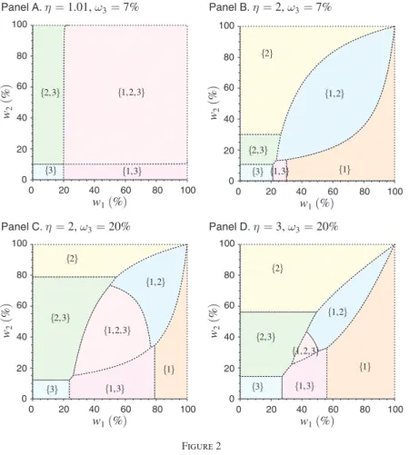
Example 4 _{(Choosing among Three Catastrophes):} We now extend Example 2 by adding a third catastrophe. Specifically, suppose that there are three potential catastrophes with τ 1 = 20% , τ 2 = 10% , and τ 3 = 5% . Figure 2 shows, for var-ious different values of _{w 3 and η , which potential catastrophes should be averted as}

w1 and w 2 vary between 0 and 1. (Figure 2 is analogous to Figure 1, except that now there is a third potential catastrophe.₎

When η is close to 1, as in panel A of Figure 2, the usual intuition applies: Catas-trophe 3 is always averted _{(since w 3 > τ 3 ), and Catastrophes 1 and 2 should be} averted if w _i > τ _i . Panel B of Figure 2 shows that this intuition fails when η = 2 ; now it is never optimal to avert all three catastrophes. In panel C of Figure 2, we increase w 3 to 20 percent , and the decision becomes complicated. Consider what happens as we move horizontally across the figure, keeping _{w 2 fixed at 50} percent. For w 1 < 30% , we avert Catastrophes 2 and 3 but not Catastrophe 1, even when _{w 1 > τ 1 = 20% . The reason is that the additional benefit from} including Catastrophe 1, ( w 1,_2, 3 − w 2,₃ )/(1 − w 2,₃ ) , is less than the cost, τ 1 . If w 1 > 30% , the additional benefit exceeds the cost, so we should avert Catastrophe 1. But when w 1 is greater than 70 percent (but less than 90 percent), we should avert Catastrophes 1 and 2, but not 3; the additional benefit of also averting Catastrophe 3, i.e., ( w 1,_2, 3 − w 1,₂ )/(1 − w 1,₂ ) , is less than the cost, τ 3 . Finally, when we increase η to 3, in panel D of Figure 2, the range of values of w 1 and w 2 for which all three catastrophes should be averted is much smaller.

We now show that the presence of many small potential catastrophes raises the hurdle rate required to prevent a large one.

Example 5 _{(Multiple Small Catastrophes Can Crowd Out a Large Catastrophe):} Suppose that there are many small, independent, catastrophes, each with cost k and benefit b , and one large catastrophe with cost K and benefit B . Then we must compare

max

m

  _{1 + mb ______}

(

)

Ignoring the integer constraint, and assuming that it is optimal to eliminate at least one small catastrophe, the optimized values of these problems are

b (1 + k) 1/b _________ e log (1 + k) and b _{(1 + k)} (1+B)/b ______________ e(1 + K) log (1 + k) ,

respectively. It follows that we should eliminate the large catastrophe if and only if (20) _________B

log (1 + K) > ________ log (1 + k) b .

Thus the hurdle rate for elimination of the large catastrophe is increased by the pres-ence of the small catastrophes.

Figure 3 shows this graphically. Here η = 4 and the small catastrophes, indi-cated on each figure by a small solid circle, have _{w i = 1% and τ i = 0.5% (on the} left) or w _i = 1% and τ _i = 0.25% (on the right). If the large catastrophe lies in the shaded region determined by _{(20), it should not be averted. In contrast, absent the} small catastrophes, the major one would be averted if it lies anywhere above the dashed 45 -degree line.

Example 6 _{(Choosing among Eight Catastrophes):} Figure 4 shows some numer-ical experiments. Each panel plots randomly chosen (from a uniform distribution on [0, 50%] ) WTPs and costs, w i and τ i , for eight catastrophes. Fixing these w i s and τ i s,

0 20 40 60 80 100 0 20 40 60 80 100 w1 (%) w2 ( % ) {3} {1, 3} {1, 2, 3} {2, 3} Panel A. η = 1.01, ω3 = 7% 0 20 40 60 80 100 0 20 40 60 80 100 w1(%) w2 ( % ) {3} {1} {1, 2} {2} {1, 3} 0 20 40 60 80 100 0 20 40 60 80 100 w1(%) w2 ( % ) {3} {1, 3} {1} {1, 2, 3} {1, 2} {2, 3} {2} 0 20 40 60 80 100 0 20 40 60 80 100 w1 (%) w2 ( % ) {3} {1, 3} {1} {1, 2, 3} {1, 2} {2, 3} {2} Panel B. η = 2, ω3 = 7% Panel C. η = 2, ω3 = 20% Panel D. η = 3, ω3 = 20% {2, 3} Figure 2

Notes: There are three catastrophe types with τ 1 = 20%, τ 2 = 10% , and τ 3 = 5%. Different panels make differ-ent assumptions about w 3 and η . Numbers in brackets indicate which catastrophes should be averted for different values of w 1 and w 2 .

we calculate _{B i and K i for a range of values of η . We then find the set of catastrophes} that should be eliminated to maximize (16). These are indicated by dots in each panel; catastrophes that should not be eliminated are indicated by crosses. The 45 º line is shown in each panel; points below it have w _i < τ _i and hence should never be averted. Points above the line have _{w i > τ i , so the benefit of averting exceeds the} cost. Even so, it is often not optimal to avert.

Panel A of Figure 4 shows that when _{η is close to 1, every catastrophe above the} 45 º line should be averted, consistent with Result 5. As η increases above 1.2, the optimal project selection depends in a complicated way on the level of risk aver-sion. When η = 5 , it is optimal to avert just one “doomsday” catastrophe. When η = 4 , it is optimal to avert two different catastrophes. When η = 3 , three should be averted—but still not the doomsday catastrophe. As η declines further, it again becomes optimal to avert the doomsday catastrophe.

IV. Extensions

Thus far, we have made various assumptions to keep things simple. We have taken an “all-or-nothing” approach in which a catastrophe is averted entirely or not at all. We have assumed that a policy to avert catastrophe A has no effect on the like-lihood of catastrophe B. And we have assumed that catastrophes are, well,

catastro-phes: that is, bad news. This section shows that all three assumptions are inessential. We can allow for partial, as opposed to total, alleviation of catastrophes; we can allow for the possibility that a policy to avert _{(say) nuclear terrorism decreases the} likelihood of bioterrorism; and we can use the framework to consider optimal poli-cies with respect to potential bonanzas—projects such as blue-sky research or infra-structure investment that increase the probability of something good happening (as opposed to decreasing the probability of something bad happening_).

10 8 6 4 0 2 w ( % )

Panel A. wi = 1% and τi = 0.5% Panel B. wi = 1% and τi = 0.25%

0 2 4 6 8 10 10 8 6 4 0 2 w ( % ) 0 2 4 6 8 10 τ (%) τ (%) Figure 3

Notes: Illustration of Example 5. The presence of many small catastrophes _{(each with cost τ} i and WTP w i , indicated

by a solid circle) expands the region of inaction for a larger catastrophe, which should not be averted if its cost τ and WTP w lie in the shaded region.

A. Partial Alleviation of Catastrophes

As a practical matter, the complete elimination of some catastrophes may be impossible or prohibitively expensive. A more feasible alternative may be to reduce the likelihood that the catastrophe will occur, i.e., to reduce the Poisson arrival rate λ . For example, Allison (2004) suggests that the annual probability of a nuclear terrorist attack is _{λ ≈ 0.07 . While reducing the probability to zero may not be} pos-sible, we might be able to reduce λ substantially at a cost that is less than the benefit. Should we do that, and how would the answer change if we are also considering reducing the arrival rates for other potential catastrophes?

Our analysis of multiple catastrophes makes this problem easy to deal with. We consider the possibility of reducing the arrival rate of some catastrophe from λ to λ(1 − p) , which we call “alleviating the catastrophe by probability p .” We write w 1 ( p) for the WTP to do just that for the first type of catastrophe. Thus w 1 , in our earlier notation, is equal to _{w 1 (1) .}

+ + + + + + + + + + + + + + + + + + + + + + + + + + + 0 30 40 wi ( % ) Panel A. η ∈ [1, 1.1] 20 10 10 20 30 40 τi(%) 0 30 40 wi ( % ) Panel B. η ∈ [1.2, 1.4] 20 10 10 20 30 40 τi(%) 0 30 40 wi ( % ) Panel C. η ∈ [1.5, 2.8] 20 10 10 20 30 40 τi(%) 0 30 40 wi ( % ) Panel D. η ∈ [2.9, 3.9] 20 10 10 20 30 40 τi(%) 0 30 40 wi ( % ) Panel E. η ∈ [4, 4.6] 20 10 10 20 30 40 τi(%) 0 30 40 wi ( % ) Panel F. η ∈ [4.7, ∞] 20 10 10 20 30 40 τi(%) Figure 4

We consider two forms of partial alleviation. First, suppose there are specific pol-icies that alleviate a given catastrophe type by some probability; an example is the rigorous inspection of shipping containers. This implies a discrete set of policies to consider, and the previous analysis goes through essentially unmodified. Second, we allow the probability by which the catastrophe is alleviated to be chosen optimally. Perhaps surprisingly, the discrete flavor of our earlier results still holds, and those results are almost unchanged.

Discrete Partial Alleviation.—To find the WTP to alleviate the first type of catastrophe by probability p , that is, w 1 (p) , we make use of a property of Poisson processes. We can split the “type-1” catastrophe into two subsidiary types: 1a (arriv-ing at rate λ 1a ≡ λ 1 p ) and 1b (arriving at rate λ 1b ≡ λ 1 (1 − p) ).14 Thus we can rewrite the CGF _{(10) in the equivalent form:}

κ(θ) = gθ + λ _{}1a  

(

)

type 1a, arriving at rate λ 1a

+ λ _{}1b  E e −θ ϕ 1 − 1

type 1b, arriving at rate λ 1b

  +

∑

(

)

all other types

 ,

so that alleviating catastrophe 1 by probability p corresponds to setting λ 1a to zero, and alleviating catastrophe 1 by probability 1 _{− p corresponds to setting λ 1b to zero.} This fits the partial alleviation problem into our framework. For example, Result 1 implies that 1 _{+ (1 − w 1 (1))} 1−η _{= (1 − w}

1 ( p)) 1−η + (1 − w 1 (1 − p)) 1−η , and the argument below equation (13) implies that w 1 ( p) + w 1 (1 − p) > w 1 (1) for all

p ∈ (0, 1) . For example, w 1 ₍ _₂1 ₎ > _1₂ w 1 (1) ; the WTP to reduce the likelihood by one-half is more than one-half of the WTP to eliminate it entirely.

More generally, we can split each type of catastrophe into two or more subtypes. Suppose Catastrophe 2 can be alleviated by 20 percent at some cost, and by 30 per-cent at a higher cost, but it cannot be fully averted. We can split this into type 2a arriving at rate 0.2 × λ 2 , which can be averted at cost τ 2a < 1 ; type 2b arriving at rate 0_{.3 × λ 2 , which can be averted at cost τ 2b < 1 ; and type 2c, arriving at rate} 0.5 × λ 2 , which cannot be averted.

To summarize, our framework can accommodate without modification policies that alleviate catastrophes by some probability, if catastrophe types are defined appropriately.

Optimal Partial Alleviation.—Now we allow the probability by which a given catastrophe is alleviated to be chosen freely. We assume that for each catastrophe i we are given the cost function _{τ i ( p) associated with alleviating by probability p . For} 14 _{The mathematical fact in the background is that if we start with a single Poisson process with arrival rate λ ,} and independently color each arrival red with probability p and blue otherwise, the red and blue processes are each Poisson processes, with arrival rates λp and λ(1 − p) , respectively.