AXCIS: Rapid Processor Architectural
Exploration using Canonical Instruction Segments
by
Rose F. Liu
S.B., Massachusetts Institute of Technology (2004)
Submitted to the Department of Electrical Engineering and Computer
Science
in partial fulfillment of the requirements for the degree of
Master of Engineering in Electrical Engineering and Computer Science
at the
MASSACHUSETTS INSTITUTE OF TECHNOLOGY
September 2005
©
Massachusetts Institute of Technology 2005. All rights reserved.
A u th o r ...
Department of Electrical Engineering and Computer Science
August 16, 2005
Certified by...
~~Krste Asanovid
Associate Professor
Thesis Supervisor
Accepted by...
... .'A 4 . .. . . . . ... C. . S... Arthur C. SmithChairman, Department Commit,tee on Graduate Students
MASSACHUSETTS INS E. OF TECHNOLOGY
AXCIS: Rapid Processor Architectural Exploration using Canonical
Instruction Segments
by
Rose F. Liu
Submitted to the Department of Electrical Engineering and Computer Science on August 16, 2005, in partial fulfillment of the
requirements for the degree of
Master of Engineering in Electrical Engineering and Computer Science
Abstract
In the early stages of processor design, computer architects rely heavily on simulation to explore a very large design space. Although detailed microarchitectural simulation is effective and widely used for evaluating different processor configurations, long simula-tion times and a limited time-to-market severely constrain the number of design points explored. This thesis presents AXCIS, a framework for fast and accurate early-stage de-sign space exploration. Using instruction segments, a new primitive for extracting and representing simulation-critical data from full dynamic traces, AXCIS compresses the full dynamic trace into a table of canonical instruction segments (CIST). CISTs are not only small, but also very representative of the dynamic trace. Therefore, given a CIST and a processor configuration, AXCIS can quickly and accurately estimate performance metrics such as instructions per cycle (IPC). This thesis applies AXCIS to in-order superscalar processors, which are becoming more popular with the emergence of chip multiproces-sors (CMP). For 24 SPEC CPU2000 benchmarks and all simulated configurations, AXCIS achieves an average IPC error of 2.6% and is over four orders of magnitude faster than conventional detailed simulation. While cycle-accurate simulators can take many hours to simulate billions of dynamic instructions, AXCIS can complete the same simulation on the corresponding CIST within seconds.
Thesis Supervisor: Krste Asanovid Title: Associate Professor
Acknowledgments
First, I would like to thank Krste Asanovi6 for being such a dedicated and supportive ad-visor. I am immensely grateful for his invaluable guidance and encouragement throughout this work.
I would like to thank Pradip Bose, at IBM Research, for introducing me to the field of processor simulation. During my summers at IBM, he has been a wonderful mentor, providing me with the skills and knowledge to pursue this work.
I also would like to thank the members of the SCALE Group for all their help and
sup-port. I would like to thank my parents, Francis and Chia, for their love and encouragement. And finally, I would like to thank Vladimir for being the best husband I could ask for.
This work was supported by an NSF Graduate Fellowship and the DARPA HPCS/IBM PERCS project number W0133890.
Contents
1 Introduction
2 Related Work
2.1 Reduced Input Sets ...
2.2 Sam pling . . . .
2.3 Synthetic Trace Simulation . . . . 2.4 Analytical Modeling . . . .
2.5 AX CIS . . . .
3 AXCIS Framework
3.1 Overview . . . .
3.2 Dynamic Trace Compression . . . .
3.2.1 Identifying Instruction Segments . . . .
3.2.2 Instruction Segment Anatomy . . . .
3.2.3 Creating the Canonical Instruction Segment 3.2.4 CIST Data Structure . . . .
3.2.5 Dynamic Trace Compression: An Example
3.3 AXCIS Performance Model . . . . 3.3.1 Data Dependency Stalls . . . .
3.3.2 Primary-Miss Dependency Stalls . . . .
3.3.3 Control Flow Event Stalls . . . . 3.3.4 Program-Order Dependency Stalls . . . . .
3.3.5 Calculating Net Stall Cycles . . . .
13 15 16 16 17 18 18 19 . . . . 19 . . . 2 2 . . . 2 2 . . . 2 5 Table . . . 29 . . . 3 2 . . . 3 3 . . . 3 4 . . . 3 5 . . . 3 6 . . . 3 7 . . . 3 8 . . . 4 0
3.3.6 Calculating IPC . . . . 3.4 Stall Calculation during Dynamic Trace Compression . . . .
4 Evaluation
4.1 Experimental Setup . . . . 4.2 R esults. . . . . 4.2.1 AXCIS Accuracy . . . .
4.2.2 AXCIS Performance Model Simulation Speed
4.2.3 CIST Size . . . . 43 43 46 . . . 46 51 52
5 Alternative Compression Schemes
5.1 Compression Scheme based on Instruction Segment Characteristics . . . . 5.2 Relaxed Compression Scheme . . . .
5.3 Optimal Compression Scheme for each Benchmark . . . .
6 Conclusion 6.1 Summary of Contributions .. .. . . . .. . . . . 6.2 Future W ork . . . .. .. . . . .. . . . . 6.3 Additional Applications. . ... . . .. . . . .. . . . . 40 41 55 56 58 61 69 69 70 70
List of Figures
3-1 Top level block diagram of AXCIS. . . . 20
3-2 Example of an instruction segment . . . 21
3-3 Example of two overlapping instruction segments. . . . 21
3-4 Class of machines supported by AXCIS . . . 22
3-5 Instruction entry format. . . . 26
3-6 Anatomy of an instruction segment. . . . 27
3-7 Sample dependencies recorded for different instruction types. . . . 28
3-8 Example of a CIST. . . . 33
3-9 CIST building example. . . . 34
3-10 Structural occupancies for each CIST entry. . . . 38
4-1 Absolute IPC errors for 19 benchmarks and 12 configurations. . . . 47
4-2 IPC errors of (a) applu, (b) f acerec, (c) galgel, and (d) mgrid for each configuration. ... ... 48
4-3 Absolute IPC error for 3 configurations with various latencies. . . . 50
4-4 Normalized APM execution time vs. normalized number of CIST entries. 52 4-5 Number of CIST entries and average APM execution times . . . 53
4-6 Number of instruction entry references in each CIST. . . . 54
5-1 Comparison of the IPC errors obtained under the characteristics-based and limit-based compression schemes. . . . 57
5-2 Comparison of the number of CIST entries obtained under the characteristics-based and limit-characteristics-based compression schemes . . . 58
5-3 Comparison of the number of instruction entry references within a CIST,
obtained under the characteristics-based and limit-based compression schemes. 59 5-4 Number of CIST entries obtained under the relaxed and limit-based
com-pression schem es. . . . 60
5-5 Number of instruction entry references in each CIST obtained under the relaxed and limit-based compression schemes. . . . 61
5-6 Absolute IPC error obtained under the relaxed compression scheme. . . . . 62 5-7 Number of CIST entries and average APM execution times obtained under
the relaxed compression scheme. . . . 63
5-8 Number of instruction entry references in each CIST obtained under the
relaxed compression scheme. . . . 64
5-9 Absolute IPC error for each benchmark obtained under its optimal
com-pression schem e. . . . 65
5-10 Number of CIST entries and average APM execution times obtained under
the corresponding optimal compression scheme. . . . 66
5-11 Number of instruction entry references in each CIST obtained under the
List of Tables
3.1 Processor configuration parameters supported by AXCIS. . . . . 23
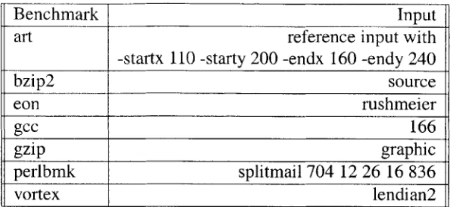
3.2 Mapping of icache and branch prediction status flags to control flow event stalls. . . . 3 9 4.1 Inputs used for benchmarks with more than one reference input. . . . 44
4.2 Minimum and Maximum processor parameters used by the DTC to gener-ate the limiting configurations. . . . 44
4.3 Twelve simulated configurations that span a large design space. . . . 45
4.4 Functional unit latency parameters. . . . 45
4.5 Cache, memory, and branch predictor configurations. . . . 46
4.6 Three simulated configurations with various functional unit and memory latencies. . . . 49
Chapter
1
Introduction
In the early stages of processor design, computer architects are faced with exploring a very large design space, which may include thousands of microarchitectural configurations. Cycle-accurate simulation is effective and widely used for evaluating different processor configurations. However, the long simulation times of these detailed simulators, along with a limited time-to-market, severely constrain the number of design points explored.
Current detailed simulators are over thousands of times slower than native hardware. For example, the popular simulator sim-outorder, of the SimpleScalar tool set [2], simulates at around 0.35 MIPS on a 1.7 GHz Pentium 4 [1]. Depending on the
bench-mark size and level of simulated detail, simulation time for one run varies from hours to weeks. Not only are the processors and memory systems modeled becoming more com-plex, additional design constraints are also being introduced for next generation processors such as power, temperature, and reliability, making simulators even more detailed. Also, benchmarks are growing in size and complexity to match those of real-world applications. For example, some benchmarks in the SPEC CPU2000 [12] suite have more than 300 bil-lion dynamic instructions. The additional complexity in both benchmarks and simulators exacerbates long simulation time, further limiting design space exploration.
Because simulation time is a function of the dynamic program size, researchers have proposed various techniques to decrease the number of simulated dynamic instructions. These techniques include reduced input sets [6], sampling [13, 10], reduced traces [4], and statistical simulation [3, 9, 8]. The reduced input set technique modifies the input data,
while sampling selectively simulates important sections of the dynamic instruction stream. Statistical and reduced-trace simulation use short synthetic traces that are generated after profiling the original dynamic trace. However, many of these techniques experience high errors, in comer cases, because these reduced programs are missing simulation-critical data. Therefore the challenge is to extract all data that affect simulation accuracy from the full dynamic trace. A simulation technique that processes only this critical subset will minimize simulation time without sacrificing accuracy.
We introduce instruction segments as a new primitive for extracting and representing simulation-critical data from full dynamic traces. Simulation-critical data contained in instruction segments include original dynamic instruction sequences as well as microarchi-tecture independent and microarchimicroarchi-tecture dependent characteristics. We also present AX-CIS (Architectural eXploration using Canonical Instruction Segments), a new framework for fast and accurate early-stage design space exploration. AXCIS abstracts each dynamic instruction and its microarchitecture independent/dependent contexts into an instruction segment. AXCIS then uses a compression scheme to compress the instruction segments of the full dynamic trace into a table containing only canonical instruction segments (CIST
-Canonical Instruction Segment Table). CISTs are not only small, but also very represen-tative of the full dynamic trace. Therefore, given a CIST and a processor configuration,
AXCIS quickly and accurately estimates performance metrics such as instructions per
cy-cle (IPC). We propose AXCIS as a complement to detailed simulation. Because CISTs can be reused to simulate many processor configurations, AXCIS can quickly identify regions of interest to be further analyzed using detailed simulation. In this work, we apply AXCIS to in-order superscalar processors. In-order processors are becoming more popular with the emergence of chip multiprocessors (CMP), which have stricter area and power constraints and emphasize thread-level throughput over single threaded performance.
This thesis is structured as follows. Chapter 2 provides an overview of related works on efficient simulation techniques. Chapter 3 describes the AXCIS framework and instruction segments in detail. Chapter 4 evaluates AXCIS for accuracy and speedup, in comparison with a cycle-accurate simulator. Chapter 5 proposes alternative compression schemes for
Chapter 2
Related Work
In large design space studies, architects may need to simulate and compare thousands of processor configurations. Since detailed simulation is too slow to complete these studies in a timely manner, much work has been done on reducing processor simulation time. Many previously proposed techniques decrease simulation time by reducing the number of dynamically simulated instructions. These techniques include reduced input sets, sampling, and synthetic trace simulation. Another approach to improving simulation time is analytical modeling, which does not involve any simulation to evaluate different configurations once the analytical equations have been specified.
All these efficient simulation techniques produce results that approximate those
ob-tained using detailed simulation. These techniques are usually evaluated based on the ab-solute and relative accuracies of their approximations. Abab-solute accuracy, which is harder to obtain than relative accuracy, refers to the technique's ability to closely follow the values measured by the detailed simulator. Relative accuracy refers to the technique's ability to produce results that reflect the relative changes across a variety of processor configurations. While absolute accuracy requires the absolute errors of the approximations to be small, rel-ative accuracy can be obtained when the error is consistently positive or negrel-ative over a broad range of configurations. Configuration dependence also plays a role in evaluating the accuracy of these techniques. Configuration independent techniques produce results with similar error regardless of the simulated configuration, while the error of configuration de-pendent techniques vary depending on the simulated microarchitecture, making it difficult
to compare configurations.
2.1
Reduced Input Sets
Reduced input sets such as MinneSPEC [6] modify the reference input set to reduce simulation time. Because the dynamic instruction sequence generated using reduced in-put sets can be very different from that generated using reference inin-put sets, the re-duced input set technique cannot provide absolute accuracy but relative accuracy may be achieved. Ideally, since the entire program is simulated, the dynamic execution characteris-tics obtained from reduced and ref erence input sets should track. Therefore simulation results from a reduced input set should correlate to those obtained from the corresponding ref erence input set. However, as shown by Yi et al., the relative accuracy of the reduced input set technique is poor [14]. Yi et al. also shows that the accuracy of reduced input sets varies widely, depending on the simulated configuration. Therefore, low accuracy as well as configuration dependence make reduced input sets less appropriate for design space ex-ploration.
2.2 Sampling
Sampling performs detailed simulations on selected sections of a benchmark's full dynamic instruction stream, while functionally simulating the instructions and warming the microar-chitectural structures before and between these selected sections. Functional simulation and warming is needed to eliminate cold-start effects, to improve the accuracy of data gath-ered during detailed simulation. Two popular sampling techniques are SimPoint [10] and SMARTS [13]. SimPoint is based on representative sampling, which attempts to extract a subset of the benchmark's dynamic instructions to match its overall behavior. SimPoint uses profiling and statistically-based clustering to select representative simulation points.
After simulation, SimPoint weighs the results from each simulation point to calculate the final results. SMARTS is based on periodic sampling, where portions of the dynamic in-struction stream are selected at fixed intervals (sampling units) for detailed simulation.
SMARTS optimizes periodic sampling by using statistical sampling theory to estimate
er-ror between sampled and ref erence simulations to give recommendations on sampling
frequency. This provides a constructive procedure for selecting sampling units at a desired confidence level. To speed up functional simulation between sampling units, SMARTS only performs detailed warming of microarchitectural structures in periods before the sam-pling units. As shown by SimPoint, SMARTS and Yi et al. [14], these samsam-pling techniques have high absolute and relative accuracy and reduce simulation time. Although sampling is an efficient way of performing detailed simulation, it is still not fast enough to quickly explore large design spaces. For example, sampling techniques still have to simulate all
dynamic instructions, at various levels of detail, in order to avoid cold start effects. Also,
sampling techniques redundantly simulate branch predictors and caches when multiple pro-cessor configurations share the same cache and branch predictor settings.
2.3 Synthetic Trace Simulation
Both statistical simulation [3, 9, 8] and reduced-trace simulation [4] use profiling to cre-ate smaller synthetic traces. In statistical simulation, profiling gathers program execution characteristics to create distributions, histograms, or graphs on basic blocks, instruction contexts, dependence distances, instruction-type frequencies, cache miss rates, and branch misprediction rates. Synthetic traces are then created by statistically generating a stream of instruction types and then assigning dependencies based on the execution characteristics. These generated traces are simulated until performance converges to a value. The main drawback of statistical simulation is that the instruction sequences in these synthetic traces are not equivalent to the ones in the original dynamic instruction streams. This discrepancy can cause large errors in performance simulation. In reduced-trace simulation, profiling
gathers information about each instruction, including the previous n instructions as con-text. Instructions are then categorized, and these categories are used with the R-metric and
a graph of the program's basic blocks to generate a synthetic trace tailored towards a target
system. The configuration dependent nature of these synthetic traces make reduced-trace simulation less appropriate for large design space studies. Also, for some programs such
as gcc, reduced-trace simulation was not able to generate a representative synthetic trace.
2.4 Analytical Modeling
Analytical models abstract away detail and focus only on key program and microarchitec-ture characteristics. These characteristics are then used to compute model parameters to estimate performance. Once the analytical equations are specified, results for a particular configuration can be obtained very quickly since no simulation is involved. Noonburg and Shen [7] use probability distributions, of program and machine characteristics, in simple functions to model parallelism in control flow, data dependencies, and processor perfor-mance constraints on branches, fetch, and issue. Karkhanis and Smith [5] base their perfor-mance model on ideal IPC, using only data dependencies, and later adjust for perforperfor-mance degradation from cache and branch miss events. Analytical models are fast, generally accu-rate, and provide valuable insight into processor performance. However, these models also rely on many assumptions about the simulated microarchitecture, making them difficult to modify and adapt to new designs. Therefore they are not suitable for detailed design space exploration.
2.5 AXCIS
Like reduced input sets, sampling, and synthetic trace simulation, AXCIS also decreases simulation time by reducing the dynamically simulated instructions. First AXCIS com-presses the dynamic instruction stream, of a particular benchmark, into a CIST. During compression, AXCIS also simulates a branch predictor and caches. Once created, the
CIST can be used to simulate a large set of configurations. Therefore, unlike sampling, AXCIS does not need to simulate all dynamic instructions or re-simulate branch
predic-tors and caches for configurations sharing equivalent settings for these structures. Also, because CISTs retain the original instruction sequences, CISTs can be more representative of dynamic traces than synthetic traces. Because AXCIS is highly efficient, we propose
Chapter 3
AXCIS Framework
In this chapter, we describe the AXCIS framework and define instruction segments. In particular, we describe how AXCIS compresses the dynamic traces into CISTs and how CISTs are used to estimate processor performance.
3.1 Overview
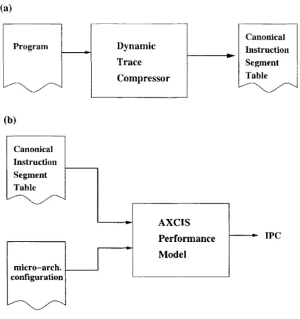
AXCIS is divided into two stages: dynamic trace compression and performance
model-ing. In the first stage, the Dynamic Trace Compressor (DTC) identifies and compresses all dynamic instruction segments into a Canonical Instruction Segment Table (CIST), as shown in Figure 3-1 (a). In the second stage, the AXCIS Performance Model (APM) calcu-lates the performance (IPC) of a particular microarchitecture given a CIST and a processor configuration, as shown in Figure 3-1 (b).
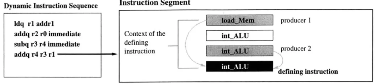
An instruction segment is defined for each each instruction in the dynamic trace. The instruction segment, of a particular dynamic instruction, consists of the sequence of instruc-tions, starting from the instruction producing the oldest dependency and ending with the dynamic instruction itself. This last instruction is termed the defining instruction of the seg-ment because the instruction segseg-ment is defined for this particular instruction. All instruc-tions in the instruction segment are abstracted into their instruction types (i.e. integer ALU, floating point multiply, etc.) because the specifics of each instruction are not needed for performance simulation. Figure 3-2 shows a sample instruction segment, whose defining
(a)
Canonical
Program Dynamic Instruction
Trace Segment Compressor Table (b) Canonical Instruction Segment Table AXCIS Performance IPC | Model micro-arch.Moe configuration
Figure 3-1: Top level block diagram of AXCIS. (a) Dynamic trace compression. (b) Per-formance modeling.
instruction is the last instruction in the portion of the dynamic trace shown. Overlapping dependencies cause the instruction segments to overlap as well, as shown in Figure 3-3. Note that we use the Alpha instruction set in all examples in this work.
A CIST contains one instance of all instruction segments defined in the dynamic trace. All CIST entries are unique, and each entry in the CIST contains an instruction segment and
a frequency count. The frequency count represents the number of segments in the dynamic trace that are canonically identical to the segment in the CIST entry. As the DTC identifies instruction segments, it compares them to existing segments in the CIST. Compression occurs when a newly identified segment is equal to an existing segment in the CIST. In this case, the DTC increments the existing segment's frequency count. If an equivalent segment is not found, the DTC adds the new segment to the CIST. The compression scheme, used
by the DTC, defines instruction segment equality. Therefore by varying the compression
ldq ri addrl producer 1
addq r2 rA immediate Context of the int ALU
subq r3 r4 immediate defining
addq r4 r3 ri instruction 1 producer 2
in______ _._defining instruction
Figure 3-2: Example of an instruction segment. A portion of the dynamic instruction se-quence is shown on the left. The instruction segment, shown on the right, is defined for the last instruction in this sequence, termed the defining instruction. The defining instruction has two dependencies, represented by arrows.
2 int.ALU
4 intALU
Figure 3-3: Example of two overlapping instruction segments. Instruction entry 5 is both a defining instruction of the first segment, as well as a producer of a value consumed by instruction entry 6.
dynamic trace.
The APM uses the structure of the CIST to perform dynamic programming to quickly estimate instructions per cycle (IPC), for a given configuration. For each instruction seg-ment in the CIST, the APM calculates the stall cycles of the defining instruction of the segment. Once the APM has calculated the stall cycles of all defining instructions in the CIST, the APM estimates IPC using the net stall cycles of the entire CIST. Note that the use of different compression schemes in the DTC does not change how the APM calculates performance.
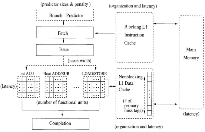
In this work, we apply AXCIS to model the class of machines shown in Figure 3-4, which include in-order superscalar processors, blocking LI instruction caches, nonblocking Li data caches, and bimodal branch predictors. More specifically, these machines include
Instruction Segment
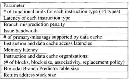
all configurations that can be described by instantiating the parameters listed in Table 3.1.
(latency):
(predictor sizes & penalty ) (organization and latency)
---Branch Predictor --- --- I lcigL Blocking L I Fetch ~Instruction Cache Issue (issue width)---4---
---nt ALU float ADD/SUB LOAD/STORE
--- Nonblocking
-- -.-- .- Ll Data
-. . . Cache
(number of functional units) (# of
__________________primary;
miss tags)
-Completion (organization and latency)
Main Memory
-lat--~
(latency)
Figure 3-4: Class of machines supported by AXCIS. All parameterizable machine
charac-teristics are drawn with dashed lines and labeled in parentheses.
3.2
Dynamic Trace Compression
Dynamic trace compression is divided into two main tasks. The first task identifies the instruction segment defined for each instruction in the dynamic trace. The second task compresses the instruction segments into a CIST.
3.2.1
Identifying Instruction Segments
All simulation-critical data relating to one dynamic instruction can be compactly
repre-sented by an instruction segment. An instruction segment contains both microarchitecture independent and dependent characteristics. Microarchitecture independent characteristics
Parameter
# of functional units for each instruction type (14 types)
Latency of each instruction type Branch misprediction penalty Issue bandwidth
# of primary-miss tags supported by data cache
Instruction and data cache access latencies Memory latency
Instruction and data cache organizations:
(# of blocks, block size, associativity, replacement policy)
Bimodal Branch Predictor table size Return address stack size
Table 3.1: Processor configuration parameters supported by AXCIS.
are inherent within the program and do not depend on machine configuration, while mi-croarchitecture dependent characteristics refer to locality characteristics that depend on cache and branch prediction architectures.
Microarchitecture Independent Data
Each dynamic instruction has associated microarchitecture independent data such as in-struction type, context, and set of data and program-order dependencies.
AXCIS categorizes the instructions into 14 types: integer ALU, integer and floating
point multiplies, integer and floating point divides, floating point add, floating point com-pare, floating point to integer converter, floating point square root, load cache access, load memory access, store cache access, store memory access, and nop.
We only consider read-after-write (RAW) data dependencies, since write-after-read (WAR) and write-after-write (WAW) hazards either do not occur or are generally elimi-nated in in-order architectures. We ignore memory address dependencies between store and load instructions because the effects of these dependencies are already modeled by the memory instruction types. In in-order machines, if a producing store instruction has not completed due to a cache miss, the consuming load instruction will also miss in the data cache. Therefore the effects of this memory dependency will be captured by the cache miss event and represented by the memory access instruction type.
In order for the APM to model structural hazards that limit issue width in multiple-issue machines, the DTC must capture the program order of dynamic instructions. This is done using program-order dependencies which form between consecutive dynamic instructions. Except for the first instruction, every instruction is dependent on its preceding instruction in the dynamic trace.
Each dynamic instruction belongs to a particular program context, which is defined by the dependencies of the instruction. The context of an instruction refers to the instruction sequence, starting from the producer of the instruction's oldest dependency and ending with the instruction itself.
Microarchitecture Dependent Data
Each dynamic instruction has associated microarchitecture dependent data such as instruc-tion cache hit/miss, data cache hit/miss, and branch predicinstruc-tion/mispredicinstruc-tion results.
The DTC simulates a branch predictor and instruction and data caches. During dynamic trace compression, only the organizations of these structures need to be specified. Latency
assignments are not needed. For caches, the DTC needs to know their sizes, associativities, and line sizes. For branch predictors, the DTC needs to know the type of branch predictor and the sizes of their associated buffers. By simulating these structures, the DTC deter-mines whether each instruction hit or missed in the instruction cache. If the instruction follows a branch, the DTC determines the type of the branch (taken/not taken) and whether or not it was correctly predicted. If the instruction is a load or store, the DTC determines if it hit or missed in the data cache. Hits in the data cache refer to both true hits as well as secondary misses. On true hits, data is found in the cache. On secondary misses, data is not yet in the cache, but a request has already been sent to fetch the line from memory. All hits in the instruction cache are true hits because we model in-order processors that block until the required instruction is fetched from memory.
In order for CISTs to be general enough to support non-blocking data caches with a varying number of outstanding misses, the DTC also records cache line dependencies and
primary-miss dependencies. Cache line dependencies form between consumers of cache
cache line. Cache line dependencies allow the APM to simulate a wide range of latencies by distinguishing between true cache hits and secondary misses, in a non-blocking data cache. Primary-miss dependencies form between two adjacent primary misses, and are used by the APM to simulate a varying number of outstanding misses, by modeling structural hazards on primary miss tags.
Because the DTC simulates caches as well as a branch predictor, the resulting CISTs can only be reused to simulate configurations sharing the same branch predictor and cache organizations. Although this constraint still allows CISTs to support a large number of configurations, CISTs can be made more general to support an even wider range of ma-chines by having the DTC simultaneously simulate multiple caches and branch predictors to create different segments for the same dynamic instruction. Then all the segments can be compressed into one multi-configuration CIST, where each CIST entry has a separate frequency count for each cache and branch predictor organization.
3.2.2
Instruction Segment Anatomy
For each dynamic instruction, the DTC identifies its corresponding instruction segment. Each instruction segment contains some data and a sequence of instruction entries to rep-resent the context of the defining instruction, which is the last instruction entry in this
sequence. The specifics of the data, stored in the segments and instruction entries, depend on the particular compression scheme used by the DTC. The following descriptions of the
instruction segment anatomy are based on the limit-based compression scheme presented in Section 3.2.3.
A sample instruction entry is shown in Figure 3-5. Each instruction entry contains the
following fields:
Instruction type - One of 14 types.
Sorted set of dependence distances - Captures all dependencies of an instruction entry.
A dependence distance refers to the number of dynamically executed instructions in
the sequence starting from the producer down to, but not including, the consumer associated with the dependency.
CIST index -CIST index of the instruction segment defined for this instruction entry.
Icache status -Hit or miss in the instruction cache.
Branch prediction status -Predicted or mispredicted during fetch. In blocking instruc-tion caches, instrucinstruc-tions that do not immediately follow branches are automatically correctly predicted because the instructions immediately following branches experi-ence all associated stall cycles. If the instruction immediately follows a branch, the type of branch (taken or not taken) is also recorded.
Min/Max stall cycles - Used by the DTC to find canonically equivalent segments. Sec-tion 3.2.3 describes this field in detail.
Type DepDistSet CIST Index Icachestat bpred-stat stalls<min, max> correct
LD_Li { 5, 9, na, na, na} 5 mss taken < 2, 10 >
Figure 3-5: Instruction entry format.
Instruction segments also contain pairs of minimum and maximum structural
occupan-cies pertaining to the defining instruction. Structural occupanoccupan-cies are snapshots of
microar-chitectural state (e.g. issue group size) at the time an instruction is evaluated for issue. The pairs of min/max structural occupancies of the defining instruction are used with the min/max stall cycles of instruction entries to identify canonically equivalent instruction segments. Figure 3-6 shows the anatomy of an instruction segment and its corresponding dynamic code sequence.
The first fi ve instruction entry fields are required for all compression schemes explored in this thesis. Only the last field (min/max stall cycles) and the min/max structural occu-pancies are specific to the limit-based compression scheme described in Section 3.2.3.
Sorted set of dependence distances
The following four types of dependencies are recorded in the dependence distance set:
Dynamic Instruction Sequence ldq ri addrl addq r2 rO immediate subq r3 r4 immediate addq r4 r -e Instruction Segment Instruction Sequence:
o producer 1 instruction entry Context of the int ALU ...
defining
instruction producer 2 instruction entry
defining instruction entry min/max structural occupancies:
issue width occupancy <min, max>: functional unit occupancy <mn, max>:
min instructions issued [1] min iALU _"
max instructions issued [L] fADD
primary-miss tag occupancy <min, max>:
min max iALU **
max fADD ...
Figure 3-6: Anatomy of an instruction segment.
2. Cache line dependency
3. Primary-miss dependency
4. Program-order dependency
All instructions referenced by the dependence distance set are included in the
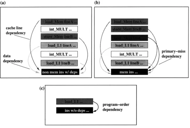
instruc-tion segment sequence. These instrucinstruc-tions as well as any intermediate instrucinstruc-tions form the context of the defining instruction of the segment. If any of the first three types of dependencies exist in a dependence distance set, the previous instruction would already be included in the instruction segment. Therefore the dependence distance set does not need to explicitly record program-order dependencies for instructions that have other dependen-cies. The dependence distance set explicitly records program-order dependencies only for instructions without other types of dependencies.
The number of elements in the dependence distance set varies between 1 and 5. Integer, floating point, and cache-hit instructions have up to 4 entries in their dependence distance sets. Up to 2 entries correspond to the producers of the operands, and up to 2 entries
cor-respond to the producers of cache line dependencies. Cache line dependencies only occur if the immediate producers are loads that hit in the cache. Cache-miss instructions have up to 5 entries in their dependence distance sets. Four of these entries are identical to the ones described above. The last entry corresponds to the producer of the primary-miss depen-dency, which is the previous primary cache miss. Except for the first dynamic instruction, instructions without any other dependency have at least the program order dependency. Figure 3-7 shows the dependencies recorded for each type of instruction.
(a)
(c)
(b)
nMULT ...__ primary-nuss
dependency
Figure 3-7: Sample dependencies recorded for different instruction types. The depen-dencies shown correspond to the defining instruction of each segment. (a) Dependepen-dencies recorded for non-memory access instructions. (b) Dependencies recorded for memory ac-cess instructions. (c) Dependency recorded for instructions with only one dependency.
In order to maintain a reasonable instruction segment length, we limit the maximum in-struction segment size by recording only dependence distances less than MAXDEPDIST.
By varying MAXDEPDIST, we can play with the inherent trade-off between accuracy
and CIST size. In general, large MAXDEPDISTs produce good accuracy but larger CISTs. Small MAXDEPDISTs leave out information from the instruction segment, and
cache line dependency data dependency int MLULT ... intMIULT ... program-order dependency
therefore produce poorer accuracy but smaller CISTs. We set MAXDEPDIST to 512. We further minimize the length of each instruction segment by pruning away non-crucial dependencies that do not cause stalls in any configuration. Primary consumers are the first instructions to experience all stalls corresponding to the producer. Secondary consumers follow primary consumers in program order, and never experience any stalls from the pro-ducer. Therefore we do not need to record the dependency of a secondary consumer.
3.2.3
Creating the Canonical Instruction Segment Table
The DTC profiles the dynamic trace one instruction at a time. For each instruction, the
DTC first identifies the corresponding instruction segment, by gathering the
simulation-critical data described above. The DTC then determines the uniqueness of the instruction segment by comparing the segment to the entries in the Canonical Instruction Segment Table (CIST). If the instruction segment is canonically equivalent to an entry in the CIST, then the frequency count of the CIST entry is incremented. If the instruction segment does not match any entry in the CIST, then it is added to the CIST. In this manner, the CIST only contains unique instruction segments. The DTC also records the total number of dynamic instructions into the CIST.
Compression Scheme and Definition of Segment Equality
Because the definition of segment equality determines when instruction segments are com-pressed, it has a large impact on the number of entries in the CIST, which affects the accuracy of AXCIS. A relaxed equality definition results in high compression but poor ac-curacy, while a strict definition results in high accuracy but poor compression. Therefore the goal is to find a canonical equality definition with the best accuracy and compression trade-off.
An ideal equality definition should compare only instruction segment characteristics that affect performance. Comparisons of other characteristics overly constrain the defini-tion and produce larger CISTs, without improving accuracy. The number of stall cycles experienced by each instruction directly affects performance. Therefore, the DTC should
compress two segments, A and B, if the stall cycles of their defining instruction are equal in all configurations to be simulated using the CIST. We define canonical equality as follows. For all configurations Z, two segments A and B are equal if
Vz E Z, Stall Cycles(A, z) = Stall-Cycles(B, z) and (3.1)
InsType(DefiningIns(A)) = InsType(Definingins(B)),
where Stall-Cycles(A, z) are the stall cycles experienced by the defining instruction of segment A in configuration z, and Ins. Type(Def ining. Ins(A)) is the instruction type of the defining instruction of segment A. The instruction type is used by the APM to calculate stall cycles, given a particular configuration.
However, because the DTC does not have full knowledge of the simulated microarchi-tecture and it is not practical to simulate all possible microarchimicroarchi-tectures, exact stall cycles cannot be determined during trace compression. Therefore, the DTC matches instruction segments based on heuristics to approximate canonical equality. We explore several com-pression schemes in this thesis. One is described in the rest of this chapter, and the others are described in Chapter 5.
Compression Scheme based on Limit Configurations
In order to get some idea of the stall cycles experienced by an instruction, the DTC simu-lates two microarchitecture configurations. We use these two configurations to approximate the set of all configurations to be simulated using the CIST. The basic intuition is that if
two segments have the same stall cycles under two very different configurations, they are more likely to have the same stall cycles under all configurations. We chose these two con-figurations to be the limiting (minimum and maximum) microarchitecture concon-figurations to be simulated using the CIST.
Using these limiting configurations and instruction segments, the DTC calculates the minimum and maximum stall cycles for each instruction. Sections 3.3 and 3.4 describe the stall calculation procedure in detail. This pair of limiting stall cycles is recorded with each instruction entry, and is the first characteristic that is compared when determining segment
equality.
The minimum and maximum stall cycles provide a range of possible stall cycles. De-pending on the configuration, the exact number of stalls experienced by an instruction can be anywhere in this range. Therefore, even if the defining instructions of two segments have identical stall pairs, there is no guarantee that their exact stall cycles are equal. There-fore, we also compare minimum and maximum structural occupancies to more accurately determine canonically equivalent segments.
Structural occupancies play a large role in determining the exact stalls seen by an in-struction. Because the DTC simulates two limiting configurations, there are two sets of structural occupancies pertaining to a defining instruction. These occupancies include:
Issue group size: an integer representing the number of instructions in the current issue
group.
Functional unit allocation: an array of integers, where each element represents the
num-ber of units allocated for a particular functional unit type, in the current issue group.
Primary-miss tag usage: an array of integers. The array size is determined by the number
of primary-miss tags in the specified data cache configuration. Each element in the array corresponds to the number of cycles before the miss tag can be re-allocated. The DTC also compares the types of the defining instructions in the segments. Dur-ing performance modelDur-ing, the APM matches latencies with instruction types, to calculate exact stalls. Therefore instruction type information must not be lost.
To summarize, two instruction segments are equal if:
1. The pairs of limiting stall cycles, corresponding to the defining instruction, are equal.
2. The pairs of issue group sizes are equal.
3. All elements in the pairs of functional-unit allocation arrays are equal.
4. All elements in the pairs of primary-miss tag usage arrays are equal. 5. The instruction types of the defining instruction in the segments are equal.
Efficient Lookup in CISTs
In order to check for canonical equivalence, each new instruction segment needs to be compared to existing CIST entries until either a match is found or all entries have been searched. Since CISTs can grow to tens of thousands of entries, the time required using a linear search algorithm is unacceptable. Therefore we hash the CIST entries into a hash table (CIST Hash Table) to speed up the lookup process. For each new instruction segment, the DTC computes its hash and only compares the segment with entries hashed to the corresponding index of the CIST Hash Table. The DTC calculates the hash of an instruction segment by computing the XOR of all characteristics that determine segment equality.
3.2.4
CIST Data Structure
CISTs compactly record simulation-critical data by exploiting the repetition of instruction segments from loops, function calls, and code re-use. Note that CISTs contain only the information needed for accurate performance simulation. CISTs cannot be used to recreate the original dynamic trace.
A CIST is essentially an ordered array of instruction segments, as shown in Figure 3-8.
CISTs have the following properties:
" Each CIST entry contains an instruction segment and its corresponding frequency
count. The frequency count indicates the number of times a canonically identical segment has been encountered in the dynamic trace.
" CIST entries are ordered based on their first occurrence in the dynamic program
trace.
" Each CIST entry introduces a new instruction to the CIST. This new instruction is
the defining instruction of the instruction segment contained in the CIST entry.
" CIST entries may refer to defining instructions of previous CIST entries.
" Because instruction segments overlap, a particular instruction may be referenced by
Index total dynamic instructions: 4 1 frequency: 1
N---=
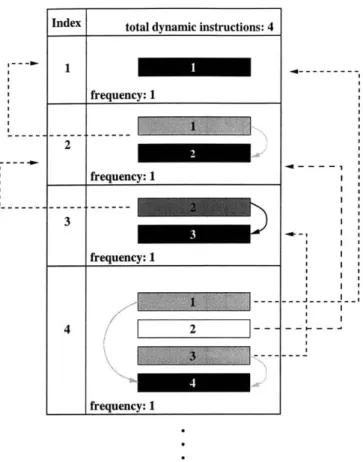
frequency: 1 -- r--ze--y:--___frequency: 1 .4---.4 - - - - 1 I I I I I I .4--I ' I * I * I I * I ~~~.1-IFigure 3-8: Example of a CIST. The instruction entries in the CIST are numbered according to their order of appearance in the dynamic trace. Using these numbers for reference, one can see that CIST entries follow program order, each CIST entry introduces one new instruction, and CIST entries overlap and point to previous entries.
3.2.5
Dynamic Trace Compression: An Example
The left side of Figure 3-9 shows a sequence of dynamic instructions, numbered in pro-gram order. The dashed lines represent dependencies between the instructions. The boxes group the instructions according to their instruction segments. For example, instruction 1 does not depend on any previous instructions and therefore is the sole instruction in the segment. Instructions 1 through 4 belong in instruction 4's segment because instruction 1 is the earliest producer of a value consumed by instruction 4. The right side of Figure 3-9 shows the CIST corresponding to this dynamic sequence of instructions. Because none of the segments shown are canonically equivalent to each other, each CIST entry has a frequency count of 1 and no compression occurs.
Dynamic Instruction Sequence
I~ I
-~
-CIST
Index total dynamic instructions: 4
1 frequency: 1 2 frequency: 1 3
=
frequency: 1 4 LZ 2 frequency: 1Figure 3-9: CIST building example.
3.3 AXCIS Performance Model
Given a CIST and a processor configuration, the APM computes performance in terms of instructions per cycle (IPC). IPC is expressed as:
IPC = Total -nstructions
TotalInstructions + CIST-Net-Stall-Cycles (3.2)
The total number of instructions is recorded in the CIST and refers to the number of in-structions profiled by the DTC. The job of the APM, is to calculate the net stall cycles experienced by the entire CIST. Note that net stall cycles may be negative for multiple-issue machines.
As mentioned earlier, stall cycles experienced by different instructions may overlap. Therefore a naive method that sums the stall cycles of individual instructions, without
/
K
I i I_-K I
\ 'modeling overlap, overestimates the total number of stall cycles and produces a pessimistic
IPC. Stall overlap is confined within the instruction segment primitive. Therefore stalls
experienced by an instruction, within some segment, cannot overlap with the stalls of an instruction outside the segment. Based on this principle, the APM accurately calculates the stall cycles of an instruction by taking into account stall cycles of preceding instructions in its segment.
The APM exploits the order-dependent nature of this algorithm by using dynamic
pro-gramming to quickly calculate the net stall cycles for an entire CIST. Because each CIST
entry introduces one new instruction, only the stall cycles of this new instruction must be calculated. The stall cycles of the other instructions in the CIST entry can be obtained from the defining instruction entries of previous CIST entries. Also, since CIST entries are created in program order, the APM can calculate the stall cycles of each new instruction sequentially, starting from the first CIST entry. Using dynamic programming, the amount of work required to calculate the net stall cycles of an entire CIST is directly proportional to the number of CIST entries. Because the number of CIST entries can be thousands of times smaller than the total dynamic instructions, the APM can simulate much faster than conventional cycle-accurate simulators.
Stall cycles are caused by the following factors: data, primary-miss, and program-order dependencies as well as control flow events. Each factor associated with an instruction results in some number of stall cycles. If an instruction is affected by more than one factor, its net stall cycles is the maximum of all its stall cycles. The APM calculates the stalls from each type of factor separately, and then takes the maximum to compute the net stalls for an instruction entry. The net stall cycles, of the entire CIST, is the sum of all defining instruc-tion entry stalls weighted by the corresponding frequency counts of their CIST entries. The following sections describe the APM's stall calculation methodology in detail.
3.3.1
Data Dependency Stalls
Data dependency stalls are caused by read-after-write and cache-line dependencies. These dependencies cause stalls when a consumer is ready to issue but its operands have not been
produced. Data dependency stalls depend on the latency of the producer, the dependence distance between the producer and consumer, and the stall cycles of all intermediate in-structions between the producer and consumer.
The stall cycles caused by one data dependency is expressed by the following equation.
DataDep-Stalls (consumer) Latency(producer) - Dep-Dist
-cn.e- Net-StallCycles(insi)
The latency of the producer is provided by the input configuration. The dependence dis-tance is recorded in the instruction entry of the consumer. The net stalls of the other instruc-tions have already been calculated by the APM and can be looked up in their corresponding instruction entries in the CIST.
For each defining instruction entry in the CIST, the APM computes all its corresponding data dependency stalls. Then the APM calculates its net data dependency stalls by taking the maximum of the stalls.
Net-DatadepStalls(consumer) = MAX(datadep-stalls1, datadep-stalls2, ---)
(3.4)
3.3.2 Primary-Miss Dependency Stalls
Primary-miss dependency stalls occur in memory access instructions that cannot issue be-cause all primary-miss tags are in use.
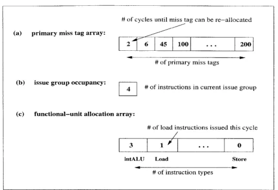
In the nonblocking data cache modeled by AXCIS, a primary-miss tag is allocated for each outstanding memory access. These miss tags are de-allocated when the memory ac-cess completes. The APM uses primary-miss tag arrays (one type of structural occupancy), shown in Figure 3-10 (a), to maintain the status of these tags. The size of the array cor-responds to the number of miss tags in the configuration, and each element represents the number of cycles until the tag becomes available. The APM creates a primary-miss tag array for each CIST entry with a memory access defining instruction. If the defining in-struction of the CIST entry has a primary-miss dependency, the values of the array are
copied from the array of the producer. If the defining instruction does not have a primary-miss dependency, all the entries in the array are initialized to -1. This indicates that all primary-miss tags are available this cycle. Memory access instructions that do not have a primary-miss dependency, are either the first memory access or the dependence distance (to the previous primary-miss) is greater than MAXDEPRDIST.
After initializing the primary miss tag array, the APM updates the array to correspond to the current cycle, instead of the cycle the producer was issued. To do this, the APM com-putes the number of elapsed cycles since the producer was issued. The number of elapsed cycles is calculated by summing the dependence distance to the producer with the net stalls experienced by all intermediate instructions (between the producer and consumer).
consumer-1
Cycles-Elapsed = DepDist + ( Net-Stall-Cycles(insi) (3.5)
i=producer+1
The APM then subtracts the elapsed cycles from each entry of the primary-miss tag array.
If no producer exists, the array remains unmodified.
Next, the APM calculates the primary-miss dependency stalls by finding the minimum value in the array. This value is the minimum number of cycles before a primary-miss tag is available.
PMDep-Stalls = MIN-ENTRY(primary-miss-tag-array) (3.6)
3.3.3
Control Flow Event Stalls
Control flow event stalls are caused by instruction cache misses, branch mispredictions, and correctly predicted taken branches.
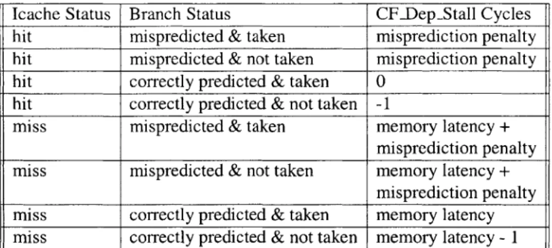
The icache and branch prediction status flags of an instruction, recorded by the DTC, directly map to the instruction's control flow event stall cycles. Table 3.2 shows the control flow stalls of an instruction based on its icache and branch prediction status flags.
Instructions that hit in the instruction cache will not experience any stalls, unless they follow mispredicted or taken branches. Mispredicted branches break the current issue
# of cycles until miss tag can be re-allocated
(a) primary miss tag array:
2 6 45 100 ... 200
# of primary miss tags
(b) issue group occupancy: # of instructions in current issue group
(c) functional-unit allocation array:
# of load instructions issued this cycle
3 1 ... 0
intALU Load Store
# of instruction types
Figure 3-10: Structural occupancies for each CIST entry.
group and cause the corresponding number of stall cycles before another useful instruc-tion can be issued. Correctly-predicted taken branches also break the current issue group, resulting in at least one stall cycle.
3.3.4 Program-Order Dependency Stalls
Program-order dependency stalls are caused by structural hazards on issue bandwidth and functional units.
The APM models issue width limitations using issue group occupancies. An issue group occupancy, shown in Figure 3-10 (b), is an integer representing the number of in-structions in the current issue group. The APM creates an issue group occupancy for each
CIST entry. The issue group occupancy of the first CIST entry is initialized to zero,
be-cause no instructions have been issued this cycle. The defining instructions of all other
CIST entries have a program-order dependency on their preceding instruction. Therefore
the issue group occupancies of these other CIST entries are copied from the entries of their producers.
Icache Status Branch Status CFDepStall Cycles hit mispredicted & taken misprediction penalty hit mispredicted & not taken misprediction penalty hit correctly predicted & taken 0
hit correctly predicted & not taken -1
miss mispredicted & taken memory latency +
misprediction penalty miss mispredicted & not taken memory latency +
misprediction penalty miss correctly predicted & taken memory latency miss correctly predicted & not taken memory latency - 1
Table 3.2: Mapping of icache and branch prediction status flags to control flow event stalls.
Structural hazards occur when too many instructions of one type are ready to issue in one cycle. AXCIS assumes that all functional units are fully pipelined. Therefore at the beginning of each cycle, all functional units are available. The APM models functional-unit structural hazards using functional-functional-unit allocation arrays, shown in Figure 3-10 (c). Each element of the array corresponds to the functional units of one instruction type. The elements contain the number of instructions, of that type, that are being issued this cy-cle. The APM creates a functional-unit allocation array for each CIST entry. Except for the first entry, the arrays of all other entries are copied from the producing CIST entry of the program-order dependency. The array, of the first CIST entry, is initialized to all ze-ros. AXCIS may be extended to model partially pipelined functional units by applying the technique used to model primary-miss tags.
The APM calculates the program-order dependency stalls, of each CIST entry, by com-paring the issue group occupancy and functional-unit array with constraints specified in the input configuration. For example, if the issue group occupancy is less than the maximum issue width, the instruction will not experience any hazards from limited issue bandwidth. Also, if the corresponding functional unit array entry is less than the number of available units of that instruction type, the instruction will not experience any functional-unit struc-tural hazards. When no strucstruc-tural hazards are detected, the program-order dependency stalls are set to -1. This indicates that the instruction issues in the current cycle. When structural hazards are detected, these stall cycles are set to 0, indicating that the instruction
issues in the next cycle.
_ -1, no structural hazards
POJDep-Stalls = (3.7)
0, structural hazards
3.3.5
Calculating Net Stall Cycles
After calculating the stalls from each type of dependency, the APM computes the net stall cycles, of a defining instruction entry, by taking the maximum of the stalls.
Net StallCycles = MAX (NetDataDep-Stalls, (3.8)
PMDepStalls, CFEventStalls, PODep-Stalls)
Then the APM issues the instruction by updating the occupancies of the correspond-ing CIST entry. If NetStallCycles is negative, the instruction issues in the current issue group. In this case, the APM increments the issue group occupancy and the corresponding functional-unit array entry. Otherwise, the instruction issues in a new group. In this sec-ond case, the APM sets the issue group occupancy and the correspsec-onding functional-unit array entry to 1. All other entries in the functional-unit array are set to 0. If the instruc-tion accesses memory, the APM makes two updates to the primary miss tag array. In the first update, the APM simulates the net stall cycles experienced by the instruction by sub-tracting these stalls from each array entry. In the second update, the APM resets the entry
containing the minimum cycles with the memory latency subtracted by 1.
3.3.6
Calculating IPC
To calculate instructions per cycle (IPC), the APM needs to first compute the net stall cycles of the entire CIST. In the previous sections we described how to calculate the net stall cycles for each defining instruction entry. To calculate the net stall cycles of the entire CIST, the APM takes the weighted sum of the stall cycles and frequency count of each CIST entry.
The stall cycles of each CIST entry correspond to the stall cycles of the defining instruction of that entry.
CIST-Size
CISTNet-StallCycles = Freq(i) * Net Stall -Cycles(Def iningIns(i))
(3.9)
With this value and the total instructions, the APM computes IPC using Equation 3.2.
3.4
Stall Calculation during Dynamic Trace Compression
The DTC computes the minimum and maximum stall cycles of each instruction using the same methodology as the APM. However, there are two main differences. The first differ-ence is that the DTC computes two stall cycle values for each dynamic instruction, using the two limit configurations. The APM computes only one stall cycle value corresponding to the input configuration. The other difference is that the DTC only computes the stall cycles for the current instruction. The APM computes the stall cycles for all defining in-structions in the CIST. Also, the APM computes the net stall cycles of the entire CIST to calculate IPC.