Axially symmetric electron beam and magnetic field systems

-T-+- AWAIT ROOM 36-412Mo1,c

saGcu Us.tts IntitUteo Tccnooehoo...

AXIALLY SYMMETRIC ELECTRON BEAM

AND MAGNETIC FIELD SYSTEMS

L. A.

HARRIS

A

TECHNICAL REPORT NO. 170

AUGUST 29, 1950

RESEARCH LABORATORY OF ELECTRONICS

MASSACHUSETTS INSTITUTE OF TECHNOLOGY

CAMBRIDGE, MASSACHUSETTS

k3

The research reported in this document was made possible through support extended the Massachusetts Institute of Tech-nology, Research Laboratory of Electronics, jointly by the Army Signal Corps, the Navy Department (Office of Naval Research) and the Air Force (Air Materiel Command), under Signal Corps Contract No. W36-039-sc-32037, Project No. 102B; Department of the Army Project No. 3-99-10-022.

MASSACHUSETTS INSTITUTE OF TECHNOLOGY

RESEARCH LABORATORY OF ELECTRONICS

Technical Report No. 170 August 29, 1950

Axially Symmetric Electron Beam and Magnetic Field Systems

L. A. Harris

This report is identical with a doctoral thesis in the Department of Electrical Engineering, M.I.T.

Abstract

The theory of longitudinally uniform and axially symmetric electron beams focused by a uniform axial magnetic field is pre-sented. It is assumed that the axial velocity is common to all electrons and that they do not cross each other radially. The radial electric, magnetic, and centrifugal forces are balanced if the proper relation between the magnetic field at the cathode and that in the uniform beam is satisfied. This balance is due to the rotation of electrons around the axis brought about by their cross-ing magnetic field lines. A general graphical method is presented for obtaining the potential distribution required for the design of hollow beams.

The necessity of bringing the beam through a transition re-gion where electrons acquire their angular velocity restricts the problem to two categories in which the cathode is either in a uni-form magnetic field or in a magnetically shielded region. Special cases are the solid beam, the hollow beam with uniform radial charge density, the hollow beam between coaxial electrodes at the same potential,and the hollow beam inside an outer electrode only. Of interest is the case of a hollow beam focused with a magnetic field in the cathode region only. Explicit design equations are presented for all cases. The possible effects of incidental ioni-zation are briefly considered.

Experimental results confirm the theory qualitatively and to a considerable extent quantitatively, and indicate the importance of the cathode flux condition and the need for a good method of bringing the beam through the transition region.

I. INTRODUCTION

This paper is a study of the theory and some means for attainment of high-density electron beams of axial symmetry. It is concerned with the general case where a beam with an arbitrary radial charge distribution is made to main-tain that distribution over a considerable distance along the axis, and the focusing is brought about by the presence of an axially symmetric magnetic field. Particular attention is paid to hollow electron beams, where the charge density is finite only between two chosen radii, and zero elsewhere.

The interest in this problem is due to the requirements of microwave vacuum tubes, almost all of which make use of an electron beam. These beams differ essentially from those used in more familiar devices, such as the cathode-ray tube, because of their much higher density, the requirement that they re-main well-collimated over a long distance, and the requirement that they have a specific and uniform axial velocity.

In the main, only the uniform rod-shaped, or solid, electron beam has been used in tubes like the klystron, traveling-wave tube, and electron-wave tube. Recent developments, though, have indicated that it might be advantageous to use hollow electron beams in certain cases. For instance, a coaxial type waveguiding structure has been suggested for the traveling-wave tube (ref. 1). Also, it is known that in the conventional helix type traveling-wave tube and

in the klystron with ungridded resonator gaps, the electrons near the axis of the beam are not efficiently coupled to the fields with which they are supposed

to interact. Elimination of this relatively useless core of electrons would decrease greatly the d-c power used in these tubes but would leave the inter-action process relatively unchanged. This increase of efficiency due to the use of a hollow beam can be an important factor in the design of high-power microwave tubes.

Although hollow beams are not extensively used at present, their future importance is anticipated here. It is felt that a good understanding of the process of magnetic focusing of dense beams is an important factor in the further advance of the microwave art. Even in the case of solid beams, which are extensively used, the general understanding of the focusing process is not as widespread as it might be. Magnetic focusing is commonly used on an

empirical basis. The results are successful but by no means efficient. A great deal of power is wasted in producing magnetic fields much more intense than they need be, if proper design methods were used.

The difficulty in focusing a dense beam over a considerable length is brought about by space-charge repulsion forces. While this problem was recog-nized and the effects analyzed as early as 1924 (ref. 2), little has been done

-1-about it except to take it into account (ref. 3). As higher density beams came into use the axial magnetic field was applied to keep them collimated. It was pretty clear that such a field would convert any undesired radial ve-locities into rotational ones and thereby limit the size of the beam. As solid beams only were used, the application of a sufficiently intense magnetic field was sure to limit the variation of beam diameter to within any limits required.

This line of reasoning soon led to the assumption, in many analyses, of infinitely strong fields which confined the electron motion to purely axial trajectories. The properties of both solid and hollow beams in infinitely intense fields have been analyzed (refs.4 and 5) and these studies are signi-ficant in that they clarify the nature of the potential distribution in the beam, and show that there are upper limits on the beam current that can be passed through drift tubes. These infinitely strong fields are never obtained, of course, and so these analyses do have a limited validity. Analyses of the interaction processes in traveling-wave tubes (ref. 6) and klystrons are also based on the assumption of axial electron trajectories, and little thought has been given to the effects of the more complicated trajectories which actually do exist (ref. 7).

Even less thought has been given to the injection of the electron beam into the magnetic field. The solenoidal properties of the magnetic field are too often neglected in this connection.

While certain special instances of magnetic focusing have been treated in the past, notably by Brillouin (refs. 8 and 9), it is only recently that any careful analysis of the subject has been done. The solid electron beam has been treated by Wang (ref. 10) who has shown the role played by the cathode position in the magnetic field. His treatment of the problem is a significant one and forms the basis for much of the analysis presented here. The equili-brium conditions in certain hollow electron beams have been derived by Samuel

(ref. 11). The cases treated by him will be shown to be special cases of those developed here.

The purpose of the present investigation is to extend the work of Wang and Samuel in a somewhat more general form with the aim of arriving at practicable design methods which make efficient use of the magnetic field. Although we are

concerned primarily with longitudinally uniform electron beams, the cathode position in the magnetic field and other end conditions are so important that considerable attention is paid to them. The aim of deriving design methods for uniform beams governs to a large extent the method of analysis and the restric-tions imposed on the problem.

II. THEORY OF INFINITELY LONG BEAMS IN MAGNETIC FIELDS

The development to be carried out in this section is concerned only with the steady-state conditions that can exist in an infinitely long electron beam system. How the beam was produced and placed in the magnetic field is another problem to be considered in a later section.

The only beams of interest here are axially symmetric and longitudinally uniform, so the appropriate coordinate system is the cylindrical one shown in

Fig. 1.

s/

It is specified that all electrodes and

poten-Z tials are independent of and z. The magnetic field, too, is axially symmetric, and in the section of the beam being considered, is uniform and in the z direction only.

Fig. 1 Cylindrical co- The velocity range of interest is low enough so

ordinate system. that we can neglect relativistic effects, or, what

is the same thing, we neglect the magnetic field due to the beam current itself. Every electron is assumed to have started with zero velocity from a cathode at zero potential.

It was indicated at the beginning of this paper that these beams would find application in microwave tubes where the axial velocity is specified. Accordingly, we confine our attention to the one special case where this velocity z, has the same constant value for every electron in the beam. This

is merely one possible mode of existence for the beam; we consider it because it is of the greatest interest and moreover has the advantage of mathematical simplicity.

The two fundamental laws, conservation of energy and conservation of angular momentum, are the basis of this analysis. Conservation of energy gives us the following familiar equation

'2 2 2 e

r + + -2+- (1)

m

where the dot notation is used to represent total time derivatives; e is the charge on the electron, -16 x 10 coulomb; m is the electron mass, 9.1 x 10 kilogram; and is the electric potential at the point in question as measured from the cathode. All units are MKS rationalized.

The problem to be solved is to determine r as a function of the time t. The solution is obtained as an integral of Eq. 1, but before this is done, the equation must be reduced to one in r alone. Setting z equal to a constant has eliminated one variable. It remains to reduce

e

and p to functions of r

only.

-3-Reduction of 0

The conservation of angular momentum is employed here. In applying this principle, care must be taken to use the correct expression for the angular

momentum of a particle in a magnetic field (ref. 8). This is conveniently done by use of the Lagrangian function L (ref. 12).

L = -eq + eA · v + -v · v (2) 2

where A is the vector magnetic potential defined by

OVxA = B; (3)

B is the magnetic flux density vector; and v is the vector velocity of the particle.

The ith component of momentum is defined by AL

ePi (4)

qi

where qi is the total time derivative of the ith coordinate of the particle. Defined in this way, Pi is not merely the mechanical momentum mv but depends on A also. The equations of motion are found by means of Euler's equation

(ref. 12).

d vco o . (5)

dt ~li aqi

The vector v is represented in the cylindrical coordinate system by

v = irr + ior + lzZ (6)

where the i_i are unit vectors.

The axially symmetric magnetic fields may be produced by currents flowing in the 8 direction and the vector potential A has a component, A, only.

Substitution of (6) into (2) yields

L = -e + eArO +(r + r z+ 2 (7)

2 and Euler's Eq. 5 for the component gives

eAgr + mr20 = constant. (8)

Equation 8 is an explicit statement of the conservation of angular mo-mentum. We used the Lagrangian and the vector potential because of the

sim-plicity of the method and the ability to express the magnetic field with a single component of A. The constant may be evaluated for any one electron by considering the conditions at the cathode at the starting point of that electron. Here the constant is eAcrc + mrc2c where the subscript c refers

to the conditions at the cathode. We have already assumed that the electron

--velocity here is zero, hence the tangential --velocity rcec, in particular, is zero. Consequently, eAer + mr 2 = eAcrc or

e/m

= 2m (rcAc - r)

r (9)

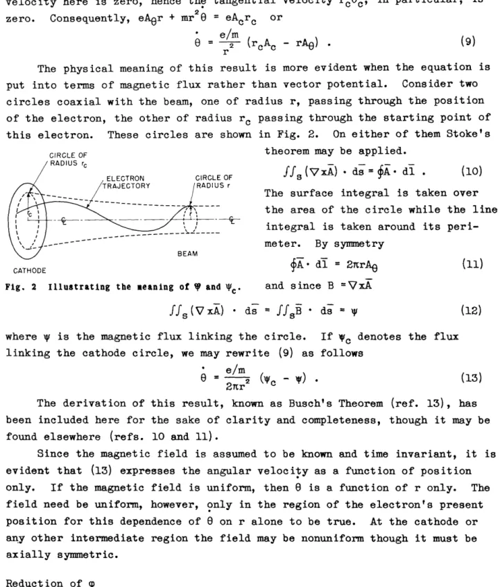
The physical meaning of this result is more evident when the equation is put into terms of magnetic flux rather than vector potential. Consider two circles coaxial with the beam, one of radius r, passing through the position of the electron, the other of radius rc passing through the starting point of this electron. These circles are shown in Fig. 2. On either of them Stoke's

CIRCLE OF theorem may be applied.

RADIUS rc) (10)

Fr.TRON CIRCLE OF PUS (VxA) d = - dl . (lo)

RAJECTORY RADIUS r

BEAM

CATHODE

Fig. 2 Illustrating the meaning of T and Wc.

The surface integral is taken over the area of the circle while the line integral is taken around its peri-meter. By symmetry

fA' dl = 2rA e (11)

and since B =V xA

ffs(VxA) ds = Bff · ds = (12)

where is the magnetic flux linking the circle. If Vc denotes the flux linking the cathode circle, we may rewrite (9) as follows

e/m

2nr 2 _{(Vc - ) (13)}

The derivation of this result, known as Busch's Theorem (ref. 13), has been included here for the sake of clarity and completeness, though it may be found elsewhere (refs. 10 and 11).

Since the magnetic field is assumed to be known and time invariant, it is evident that (13) expresses the angular velocity as a function of position only. If the magnetic field is uniform, then is a function of r only. The field need be uniform, however, only in the region of the electron's present position for this dependence of 0 on r alone to be true. At the cathode or any other intermediate region the field may be nonuniform though it must be axially symmetric.

Reduction of

In order to reduce p to a function of r only, we assume that electrons do not cross each other radially in the course of their travel down the tube. The beam is symmetrical so we can think of cylindrical shells of electrons which make up the beam. These shells may vary in radius along the length of the

-5-a

beam, but they are assumed never to intersect one another or trade positions. This assumption, which appears to be a radical one is necessary for a

conven-ient solution to the problem. The principal reason for its use is mathemati-cal simplicity, although there is some justification for it aside from this.

If we were to solve this problem exactly we should have to calculate the trajectory of each electron using the potential it experiences due to the electrodes and to all the other electrons. But each of these other electrons has its own trajectory which in turn depends on all others. The task is clearly impossible. At this point we take advantage of the fact that we know what type of solution we are seeking.

Our object is to learn how to obtain beams in which the electrons do not have much radial motion. If they do, then we are not interested in that beam. For the type of beam we are trying to achieve the potential is closely ap-proximated by that of a uniform beam which is in radial equilibrium.

If we use the potential of such a uniform beam and still allow for some radial motion, we are in effect using an average potential Ap, and neglecting any longitudinal electric fields due to variations in beam diameter.

We cannot use directly in Eq. 1 either. This procedure would assume that the entire beam stayed in equilibrium while the electron in question threaded its way in and out of the beam. The solution obtained in such a manner would have to indicate a beam with no changes in radius in order to be consistent. By assuming that electrons do not cross radially, we are enabled to use the average potential and still allow for radial variations in the entire beam. The assumption is clearly true for a beam in equilibrium and is probably a fair approximation in beams with only small variations from equili-brium. It will be shown to be true also in certain other instances.

According to the assumption, each electron shell encloses a constant amount of charge which may be considered to lie along the axis. This line charge produces a logarithmic potential around it. It is therefore possible to express the potential as experienced by the electrons in any one shell as

r

= a In - + y (14)

r_o

where ro is the radius at which the electrons of that shell experience no

radial force, their equilibrium radius. The coefficients a and y are con-stants for any one shell, but vary from shell to shell. We shall characterize the electron shells by their equilibrium radius r_o. The coefficients a and y are thus functions of r, but not of r or t. They are evaluated by means of their relationship to the average potential . When the beam is in equili-brium and must be equivalent and so must their derivatives with respect to r.

-6-DPI] = [ r

o o

F[?r~~1O

F~ 1(15)

O -~

r₀ r0

These equations are used to determine a and y and this operation is carried out in the next section after the calculation of p itself. The ex-pression for p given in (14) is not the true potential but it is the poten-tial experienced by the electron and is used in (1) to solve for the tra-jectories.

At r, becomes y, so y is the average potential at ro, while is a coefficient giving the magnitude and direction of the radial electric field.

Equilibrium and Stability Conditions

Now that e and have been reduced to functions of r we can substitute them into Eq. 1 to obtain a differential equation in r only.

r2

+ r

e/m (af - 2 + 2 =-2e[ ln

r

+ ] (16)

L2nr m r_o

As z is the same constant for all electrons it corresponds to an ac-celerating voltage V defined by

'2 e z = -2 -V (17) m Equation 16 becomes · 2 e r e ( e/ 2 r = -2- In - - 2- ( - V) ( (18) '

e

ro e/m/2) c 2 - )2 im r. in8

In the region of the beam that we are studying, the magnetic field is axial and uniform as required by the reduction of 0. Since the field has only a z component Bz, it will be permissible to denote it simply by B without fear of confusion. The flux is given by

v nEr2B (19)

and the flux c linking the cathode circle is a constant depending only on r_o. If we let e B eH - (20) and e (21) m 2n

then after expansion and substitution of the last three equations, (18) becomes

' 2 _{r = -2--} e _{a In -- -}r _{2 (y - V) ---} e _,&H 2 (22) r + 2

n

H (22)

m r₀ m r

-7-This is the differential equation of radial motion of any electron in the beam. Equation 22 may be interpreted as defining a potential trough in which the electron rides. The kinetic energy associated with radial motion is m/2 r . As Eq. 1 defines the total energy as zero, the negative of m/2 r2 may be

con-sidered as a potential energy, so far as radial motion is concerned. This is merely an arbitrary division of the total energy into potential and kinetic

terms, but it is a convenient aid in visualizing the radial motion (ref. 10). The right-hand side of (22) becomes minus infinity for r approaching either zero or infinity regardless of whether is positive or negative. Only the region in which this quantity is greater than zero is accessible to the electron in question. The magnetic field, by limiting the energy of radial motion, prevents electrons from traveling arbitrarily far from or close to the axis.

Taking the time derivative of (22) and dividing by 2r gives us the equa-tion for the radial acceleraequa-tion.

e a (23)

r = --- + - H r . (23)

mr r

We have defined r as the radius at which there is no radial force, hence r = 0 at r = ro.

e +,n 2 2

0 -- + 3 - WH ro (24)

m r O rO

Solution for fl yields

n=

Hro2 1+ 2 a (25)

IH ro

where only the positive square root is intended here and elsewhere in this paper. The negative root would indicate a reversal of direction of magnetic field between the cathode and the beam. Although this is possible, most practical configurations will not have this reversal.

It is convenient to let e/m

2 2 = K (26)

w ro

so that the flux condition may be written

2

n=

Hr

_o

+a

or

2

lc = nro B 1 + Ka. (27)

K is a negative number because of the negative electron charge. The quantity

V1

+ Ka is less than or greater than one depending on whether a is greater than or less than zero respectively. If a is positive, the electric force

-8-6

tends to move electrons toward increasing radii. In this case, for Vc to be real, K must be greater than -1. Presently we shall see that this condition guarantees that the radial motion shall be periodic; i.e. stable.

Equation 27 shows that the flux ec linking the cathode circle is less than the flux W linking the equilibrium circle of radius ro (see Fig. 2) if

the electric force is outward. This is always the case with solid beams and may be true with hollow beams too. If the electric force is inward, a con-dition which can occur only when there is an electrode inside a hollow beam, the cathode flux c must be greater than A.

The electron motion will be a stable oscillation about ro if the

equi-valent potential energy is a minimum at r, or if r is negative for r greater than ro, and positive for r less than ro. To check the stability of the

mo-tion, we take the derivative of (23) with respect to r and evaluate it at r = r _.

[5 e a 2 2 (28)

Lr

mr

-

H

(2)

Substitution of (24) into 28) yields

e a 2

L

r jr =-2 m 2 - 4 H (29)

0

As the left-hand side of (29) must be negative, dividing the right-hand side by -4 H shows that the following inequality must be true.

Ka 1 +-- > 0

2 or

Ka > -2 , (30)

In any physical arrangement, however, c must be real so that the above inequality is always satisfied. An unstable radial oscillation of the beam in the presence of a magnetic field is not possible. The instability en-countered in a beam in a field-free space may be considered as the beginning of an oscillation about r, where ro has moved out to infinity because H is

zero and K remains finite.

The above considerations of equilibrium conditions show that any general radial charge distribution is a possible stable configuration so long as the proper flux condition (27) and stability condition (30) are satisfied. This conclusion is demonstrated in an alternative way, and perhaps more explicitly, by a variational treatment of the problem presented in an appendix.

Solution of the Differential Equation

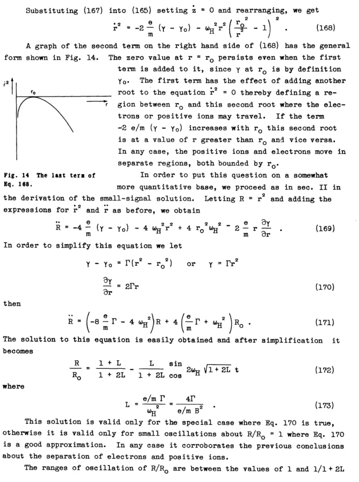
In order to solve the equation of motion (22), we make the following

-9-changes 2 r R and (31) 2 r_O = R_O then R = 2 rr and (32) R = 2 rr + 2 .

We multiply (22) by 2, (23) by 2r and add the results to obtain

R=[-2 - a - 4 - ( - V) + 4w H] -2 - a n -- 4H R . (33)

m m m R_o

The presence of the logarithmic term in (33) makes it a nonlinear differential equation. It can be solved approximately, however, by using the first term of the series expansion for n R/R_o

R R

In - = - - 1 . (34)

Ro Ro

As (34) is true only for values of R/Ro close to one, our solution will

be valid in this range only. Fortunately it is the range in which we are pri-marily interested. (For R/Ro = 1.2, or r/ro = 1.095, the error is about

10 per cent in (34).)

With this last substitution (33) simplifies to the linear equation

R = a_o + aR (35) where a[-4 e (¥V) +4 4 2 14+ K(y -V)] ao - V) + 4]1 ro [ + K - K(y m and e ~ 2 Kc al = -(4 + 2 e ) -4WH2 (1 + 2) mr 2

We multiply (35) by 2R and integrate once. 2RR = 2aoR + 2a₁RR

R =2aOR + aR + a2 (36)

The constant of integration, a2, is evaluated by substituting (22) into (36)

and setting r = r. This procedure gives

a2 = -4 Ro (1 + 2) . (37)

2

The integral of (36) neglecting the additive phase constant is

-10-R = bo + b cos 3t .

Differentiating (38) with respect to time and using the identity cos2

Pt

+ sin2 t = 1

enables us to evaluate bo, b, and 6. The results are

-I Ka _ = -2H 1 + 2 2 \l +K -(y -V)

bo =

Ro

1

(39)

1+ 2 b, = R_o (bo/Ro)2 _{- 1}

The final solution for the radius of any electron in the beam as a func-tion of time, valid only for small oscillafunc-tions, may be written

R + Ka - K (y- V)

Fl+

Ka - K(y - V) 2 2

RK = + - cos(-2H +- t)

0 1 + 1 +

--(40) If we introduce a new quantity x, defined by

b0 X 2

= 1 + - (41)

Ro 2

then (40) may be written in the neater form

R x x

- = 1 +- + x 1 + c- ost . (42)

R_o 2 4

It is apparent from (42) that as the normalized amplitude of oscillation increases so does the average radius about which this motion takes place. Figure 3 is a graph of the maximum and minimum values of R/R_o vs. the

magni-tude of the amplimagni-tude factor x. The oscillation is displaced toward the outside of Ro, the unbalance increasing with the amplitude of oscillation.

A significant point in the solution is the form of the angular frequency of radial oscillation

= -2H 1+ . 2

For stable solutions must be real as specified by (30), and since Vc is real, this is always the case.

Figure 4 is a graph showing the general form of as a function of -H which is proportional to the magnetic flux density B.

When is positive and the electric force on the particles is outward, there is a minimum magnetic field below which the oscillation is not stable.

When there is no electric force in

1.8 the radial direction ( = 0), the

1.7 - Rmax beam is in equilibrium when there

1.6 -,/ Ro is no magnetic field and it oscil-,·"1.5 lates when there is a magnetic field.

14

1.- ,,But when a is negative, remains

1.3

real even though the magnetic field

1.2

1.1 - / MEAN VLUE OF R/% becomes zero. It is thus possible,

Ro 1.0 by means of an inward electric force,

0.9 - to have a stable configuration of the

0.8 - beam with no magnetic field along its

0.7

0.6'- Rmin _ length. This case is of considerable

0.6 R_o

0.5 practical significance as it allows a

LIMITS OF OSCILLATION VS.

0.4- AMPLITUDE FACTOR X great saving in power used to produce 0.3 - R= r2 Rm"- 2- the magnetic field. It is discussed

0.2 - R ---- -2 I+2 - 4 in some detail in a later section, as

0.1- one case of special interest.

o L I I I I

0 0.1 0.2 0.3 0.4 0.5 0.6 0.7 It is necessary to check the form of X with the assumption made in

Fig. 3 Maximum and minimum radii vs. deriving it. The only questionable

amplitude factor. part of this development was the

71 1 statement that electrons do not cross

I

~

/ , 6 z 5 >- 4 3 am cr 2 Q I o

each other radially. This assumption has certain consequences not pointed

TYPICAL CURVES OF

FREQUENCY OF OSCILLATION out previously, but readily

ap-VS. LARMOR FREQUENCY

r=-2wH J1+ preciated when one examines the

be-havior of two adjacent electron

l l l l l l l l OIl

O .5 I 1.5 2 2.5 3 t 11 5

-WH ARBITRARY UNITS If one shell oscillates in

Fig. 4 Oscillation frequency vs. magnetic radius along the length of the beam,

field. then the other must do likewise, or

they will intersect. The space periods or wavelengths of these oscillations, moreover, must be the same for both shells, and the phases must be the same; when one shell expands, so must the other. A simple extension of these con-siderations leads us to the restriction that the angular frequency must be the same for all shells, hence independent of r or of Ro . This, clearly, is

not the case unless Ka is independent of r, or a is proportional to r 2 . When this is true, the solution is entirely consistent with our assumptions. This point will be discussed also in later sections, particularly the one dealing with special cases.

The assumption of noncrossing also requires that the amplitude of os-cillation be a continuous function of r_o. Though not necessarily so, this function may be monotonic with a zero value entirely inside the beam, somewhere in the charge region, or entirely outside the beam. If either the first or last possibility is true, the beam oscillates more or less as a unit, with the inside and outside edges moving in and out together. If the amplitude is zero for a value of r_o in the charge region, then the beam pulsates in thickness, the outside expanding while the inside contracts.

Although the solution we have found is not generally consistent with the assumption of noncrossing, it is conceivable that the results may still be useful. We shall always try to satisfy the equilibrium conditions in any

design. With little or no oscillation there will not be much crossing and our results may be sufficiently accurate to be useful.

It is possible too that the variation of space period across the beam will be small so that interference of the electron paths may not develop until many cycles have elapsed. In the entire length of the beam there may not be any serious radial crossing. While these considerations may give us hope for the usefulness of the general solution, its real test must come with experiment.

There is one other possibility for consistent solutions as derived here. If the axial velocity is allowed to assume different values for different electron shells, then the time period may vary while the space period remains the same for all shells. In this paper, however, we are concerned only with

the case where z and V are the same for all shells.

Angular Velocity

A consideration of the angular velocity is helpful in clarifying the physical picture of the focusing process. We return to Eq. 13

e/m

2nr2

(c - )

and the earlier definitions of dl and H (Eqs. 20 and 21) to obtain

e

-2 H (43)

r We substitute (27) into (43) to get

e =V 1+ Ka - 1 (44)

and finally, use of Eq. 42 leaves us with 1 + a

e

= _2H 2

_{- 1}

(45) + - + X + - + x l+-~cos t 2 4

-13-Evidently is a periodic quantity. If 1 +Ks is sufficiently small, the sign of alternates, otherwise fluctuates in value but retains the same sign.

The average value of is of interest. This is given by

1 2 H 2 d(Pt) 0 =

-f

0 d (t) = f 21t x x x E?~2 0 12 _{2n(l+ ) 0 1} /o _{+ x} 2_{/4 Ptx} 2 1 + x2/2 - H (46) Or integration, (46) becomes (47) The form of the average angular velocity explains the focusing action. The sign of 0 is the same as the sign of a, since both K and H are numeri-cally negative. If the electric force on an electron is outward, it encircles

the axis in such a direction as to produce an in-/,JZ ' OEQUILIBRIUM ward magnetic force, and vice versa. This average

/ '~ RADIUS

\/ ' rotation is independent of x and its magnitude

de-/

\to pends only on the relative values of electric and

magnetic fields. It is the familiar Larmor pre-cession or drift. The oscillations in radius and in angular velocity represent a motion similar to the trochoids and cycloids experienced in uniform crossed electric and magnetic fields. These paths

Fig. 5 The three possible are shown in Fig. 5. Which type of path the

elec-electron trajectories. trons follow is determined by the relative values

of 1 + Ka and x.

Since 6 is a function of Ka which is not generally independent of r, there is a rotational shearing motion between different electron shells, aside

from the oscillatory rotation. This slipping of the shells does not introduce any complication of the picture because of the axial symmetry. In the consis-tent case where a is proportional to r , the entire beam rotates as a unit.

The energy balance of the system is another point of interest. The kinetic energy of any particle is divided between axial, radial and angular velocities. At the equilibrium radius r, the potential is equal to y so the total kinetic energy must be -ey. The energy associated with the axial velocity is -eV, and the difference, -e(y - V) is associated with the

angu-lar and radial velocities. Clearly y - V must be a positive quantity, a conclusion borne out by the coefficients appearing in Eq. 40.

This energy difference has a minimum possible value that it must have to

account for the angular velocity which in turn is specified solely by the mag-netic field configuration. Any excess over this minimum means a certain

amount of radial motion. The design procedure consists of setting y - V equal to this minimum as we shall see in the section dealing with the design of the beam system.

Before we go on to consider this question, it is necessary to examine the electric potential distribution in the beam and to evaluate the coefficients a and y. This is the subject of the following section.

III. THE ELECTRIC POTENTIAL IN THE BEAM

In sec. II it was explained that the potential p as experienced by the electrons could be expressed in the form = a n r/ro + y. It was also

pointed out that in order to determine the coefficients a and y, it is nec-essary to calculate the average potential (p corresponding to a beam system uniform in the axial direction. This section is concerned with these calcu-lations and their application to the problem.

The system under consideration is axially symmetric and uniform longi-tudinally. The only variations that take place are in the radial direction.

As the most general case we assume a

N

2 ; ELECTRON BEAMS,/ hollow electron beam, coaxial with two

( cylindrical electrodes, one inside the beam, the other outside. As shown in Fig. 6, (p is the actual potential, as

Fig. 6 Hollow beam in equilibrium. measured from the cathode, applied to the

inner electrode of radius r1. The

quan-tities P2 and r2 are similarly connected with the outer electrodes; the

sub-scripts a and b refer to the inner and outer edges of the beam respectively. The charge density in the beam is a function of radius only and is de-noted by p. Its general form is

p = p(r) ra r < rb

= 0 r < ra or rb < r . (48)

Equation 48 represents a hollow beam, but can be made to represent a solid one by letting ra become zero. In that case the inner electrode must disappear and we need not concern ourselves with q1. In the same way, the

inner electrode may be removed by letting r1 become zero even if the beam

remains hollow, and the outer electrode may be removed by letting r2 recede

to infinity.

function with no singularities in the region with which we are concerned (ra _ r < rb). We may, therefore,expand p as a power series about some point in the beam say ro, (ra -- r - rb). In the charge region only, therefore

p(r) = E- pn (ro - r) (49)

n=O

Because p(r) is a physical quantity, the series of (49) is absolutely con-vergent in this range, so it may be expanded and rearranged into the form

p (r) = Pnr n (50)

n=O

where only positive integral values of n occur. Note that only p has the dimensions of charge density while Pn has the dimensions charge density/ lengthn.

The evaluation of consists of integrating Poisson's equation

(r -) (51)

r ar ar e

where e is the permittivity of free space, (1/36 x 10- 9 farads/meter), and matching the solution to the boundary conditions at r and r2. To do this,

we follow Wang (ref. 10) by letting

=T Is + L (52)

where s is a solution of (51) and L is a solution of Laplace's equation

1

a

(r L) = . (53)

r ar 8r

The sum of these two solutions must also be a solution of (51). By means of this separation we determine the individual contributions to the potential p of the charge in the beam, and of the charge on the electrodes. In the fol-lowing we shall indicate the formal process in this calculation and then give the results which are obtained when these operations are performed on the power series represented in (50).

The potential s due to space-charge alone is evaluated first. From (51) we have

a(r - ) - r

ar 'r 6

Since p is zero for values of r less than ra, we need integrate only from ra

outward. The upper limit of integration is just r, a variable radius lying somewhere in the charge region.

___

1

r r - = prdr . (54) ar E ra -16-_____ __

Only one term appears on the left since this component of the electric field is zero everywhere inside the charge ring.

Integrating (54) once more gives us the potential s for any value of r lying in the charge ring.

r

% - fs

f

prdr dr.

(55)

This time only s appears on the left because we have arbitrarily chosen Ps = 0 inside ra.

Before we can evaluate L we shall have to calculate the contribution of Ts at the outer electrode, i.e. at r2. At the outer edge of the electron

beam we have, from (55)

r

familiar logarithmic expression due to a line charge along the axis.

sine ln rb r r > rb (57) where Q is the total charge in the beam per unit length.

Q = 2n prdr. (58)

ra

The potential s can now be written for the radius r2, by substituting

(58) and (56) into (57).

- -

L

1 r + -r

f

Prd dr (59)

2 6rly I r2 r r

a a

Since 2 = TL2 + s2' we have that

r

r2 1 r

2 r

lIn

r +

-f

prd dr (60)

rb r r

and

w(PLIL =T1 (61)

because we have set s = 0 in Eq. 55. The solution for L is well known and has the following form

-L2 - TL, 1 r (62)

- n-+L . (62)

r2 r1

ln

-rl

This equation, which applies everywhere between r and r2, becomes

-17-P2 - + -lrb

f

F

pr r in- n r₂ +--f ₁r pd prdrjdrdr rr TL rL rb a *aIn - + qz (63) r2 rL in rl

when (60) is substituted into it.

Finally, the resultant potential, for any radius r in the charge region, i.e. for ra _< r < rb is given by the sum of (55) and (63).

1r b pr ln r2 1 r - _- +_{r In- +-f prdr dr} _ rL rb ra

j

r

=T a a in--r2 rt rl i r + fr~ -r prdr dr . (64) E r Lr r _a

We shall find it convenient to denote the coefficient of the logarithmic term, which is a constant of the system, by a shorter symbol, a. Thus

( = a n - + --

f

l prdrldr . (65)

r, ra r

With (50) substituted into it,

2 - q + (ln r2/rb) + - 0 (rb ( 2 n+2) 1 - Pnra + n r 2ne e O (n+2) E O n + 2 ra a = r2 in rj

This equation may be further simplified by integrating the last term by parts, which gives us

r 1 r r r r

p = a n - + Tp - - n - prdr + - pr n - dr (66)

rL e ra ra r ra

a a

Equation 66 is the required expression for the average potential at any radius in the charge region of the beam. If we substitute the power series expansion for p, (50), into this equation and perform the indicated integrations, we ar-rive at a rather unwieldy but general explicit form for , from which we can easily extract the corresponding expressions for several special cases.

- _{=P a in-} r ₊ a _{cpr ---} l n (n+ + n 2) rjLE n=o (n+2) +

1

n r n + 2 In r (67) n=O n+ 2 a r_a -18--- -18----

--.-Evaluation of a and y

The potential p expressed in the above equations applies to a uniform beam in which there is no radial motion. The potential as experienced by an electron and as used in sec. II applies when there is a radial motion in the beam provided electron shells do not cross each other. When the ampli-tude of radial oscillation is zero, or when the beam is in its equilibrium condition both and must agree, and moreover the radial electric fields derivable from and p must agree. Since = a In r/r + y, then at r = ro

where p = w

Y =[]r=r _] [ 1 _r=rO

(68) The more explicit forms of (68) are as follows

r1 rro ₁ r r y = a In - + - - In-o prdr +- pr in- dr (69) rl e ra ra ra and y = a n o + PI 1 n (ron+2_ r n+ 2) r 61 n=0 (n+ 2)2 1 n r n+ 2 ln (70) n=O n+ 2 ra

The condition on the radial electric fields at r states that

Lo:

r~~r(71)

r ro

=a] More explicitly, Eq. 71 becomes

1 ro = a-- prdr (72) ra and a Pn (ron+ 2 ra n+ 2) (73) e n=O n+2

The second term on the right of (72) represents the charge per unit length in the beam between radii ra and r. Denoting this charge by qo we may write

a = a- (74)

2Eg

from which it is seen directly that a is a function of ro which reduces to a

when r = ra. The value of a increases with r_o moreover, since qo is nec-essarily negative in an electron beam, though a itself may be either positive

-19-or negative. An equation that will be of considerable use in our design pro-cedures is derived from (72).

p(ro) = - -. (75)

In the last section it was indicated that the solution obtained is con-sistent with the assumption of noncrossing only if is a constant, and this requires a to be proportional to r_o . Equation 75 shows that this is possible only if the charge density is uniform, i.e. independent of r_o. Although the uniform charge density is a necessary condition for consistency, it is not sufficient. Integration of (75) allows the addition of a constant, which, if

2

it is not zero, does not allow a to be proportional to ro . This constant is

embodied in a and in the lower limit of integration in Eq. 72. In the case of a solid beam it is zero and the frequency is constant, but for hollow beams, very special conditions are required to bring about the appropriate a, as might be imagined from the definition of a in Eqs. 64 and 65. In a later

section this will be one of several special cases considered in detail.

With this background we shall proceed to a discussion of design procedures for this part of the beam system.

IV. A GENERAL METHOD FOR THE DESIGN OF THE INFINITE BEAM

This section is concerned with the methods of designing beam systems of the type discussed previously. The same restrictions apply here as elsewhere, and we treat only the longitudinally uniform section of the system without re-gard to the end conditions.

The design equations are nothing more than rearrangements of some of those appearing in the preceding two sections. To arrive at the most useful forms, we should consider our objective. Ordinarily the quantities predeter-mined by other considerations are the beam velocity, beam current and beam dimensions. Usually some of the following are also specified while the others must be chosen properly: radial charge or current distribution, electrode voltages, electrode geometry, and magnetic field configuration (cathode flux condition). The intensity of the magnetic field is usually a controllable quantity while its geometry may or may not be fixed by the particular application.

In choosing the quantities at our disposal, our object is to satisfy the equilibrium conditions of the beam, thereby minimizing the radial oscillation. We want to produce a longitudinally uniform beam, like that shown in Fig. 6, in which all electrons travel on constant radius paths with a common axial velocity.

--The end conditions of such a beam are of vital importance in its attain-ment. Not only the cathode flux condition, but other restrictions have to be satisfied in the cathode region and any other places where the magnetic field is not axial and uniform. While the parameter adjustments to be discussed in this section are not sufficient to guarantee equilibrium, they are necessary. The end conditions that must also be satisfied are considered separately in the next section. Here we shall assume that these end conditions are appro-priate and that the cathode flux condition is satisfied.

To find the equilibrium state, we return to the results of sec. II. From (42) we see that the amplitude of oscillation is zero if

x =0. (76) But x = 2(bo/Ro - 1) or 2 -2K(y - V) -

(

+ 1)2 x . (77) 2 + Ka

Setting x = 0 and solving for the optimum value of y - V gives us

rl + K - 1)2

(y - ) -2K (78)

There is no danger that the denominator in (77) will be zero as the real character of Wc guarantees that K is always greater than -1, as was pointed out in the discussion of stability.

Equation 78 is the necessary equilibrium condition. It could have been derived directly from the differential Eq. 22 by setting r = r_o and r = 0 and then applying the cathode flux condition (27). This emphasizes that (78) already embodies the assumption that (27) is satisfied. As we expect,

(y - V)opt. is a positive quantity.

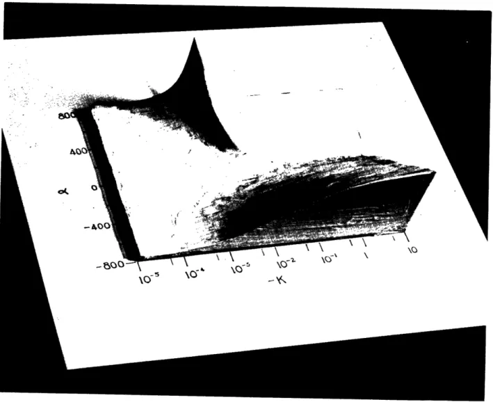
This equation has a geometrical interpretation that allows a relatively easy visualization of the design process. It may be represented by a single surface. A plaster model of this surface is shown in Fig. 7. The height represents the value of (y - V)opt. on a linear scale, and the other two coordinates represent a on a linear scale and -K on a logarithmic one. The reasons for using these particular scales will become apparent in the dis-cussion that follows.

For any one electron shell to remain in equilibrium its corresponding values of K, a, and y - V must satisfy (78) or the point represented by these constants must lie in the surface. If the entire beam is to remain in equili-brium, every representative point has to lie in the surface.

-21-_5 \ \ I

\O- \O

Fig. 7. odel of surface defined by Eq. 78.

Now consider any two shells in the beam, say the inside and outside edges. Reference to Eq. 71 shows that for the inside edge

a = a ₍₇₉₎

and for the outside edge

ab = a - - . ₍₈₀₎

2ie The difference between these two values of a is

Q b - a

~

=

2Ee (81)

and depends on the total charge per unit length between the two shells. It is therefore fixed by the beam parameters alone. This constant _{difference is} always a positive quantity for electron beams and is not affected _{by the actual} values of the a's.

-22-I _

_

.

-4O(

A similar statement may be made about the y's for the two shells in ques-tion. For the inner edge

Ya = a n a + P (82)

rL

from Eq. 69. Similarly, if we use the power series expansion for the charge density co a n +nT₀ Pn (rbn+2 - n+ 2 ) Yb = (n+ )2 b ra n ri n=O 2

+n

Pnr n+ 2 n rb (83) n=O n+ 2 a ra

The difference between these values is

b n+ 2 ra r_a

co

- = ( 2(rbn+2 (rb 2 n 2) (84)

which is also unaffected by the particular value of either of the y's. This difference is not solely dependent on the beam parameters, however, as the constant a involves the dimensions of the electrodes as well as those of the beam itself. Once the beam and electrode geometries are chosen, the differ-ence expressed in (84) is specified. From the definition of K

e/m K

2 2

WH ro

it is apparent that the ratio of the two values of -K is a constant set by the beam geometry alone

2

'Ka Trb (85)

-Kb ra

as H is the same for both shells. The difference between the logarithms of the -K's is thus a constant.

When these three differences, expressed in (81), (84), and the last statement, are taken together and interpreted geometrically in the same sense that defined the surface of Fig. 7, they define a rectangular prism or block of dimensions fixed by the beam parameters and the geometry of the system. The representative points for the inner and outer edges of the beam lie at opposite ends of a diagonal of this prism as illustrated in Fig. 8. The de-sign procedure is now clear. It consists of moving the prism about in the coordinate space until the end points of the diagonal lie in the surface

-23-simultaneously. The final position is then used

Kb, Ob, Yb r1 ,,'1,. _ _ _ _ 4. I -- -I - -- 4l U_ _ --- 4- . - -P- -1 .

UV ULs.KUI4U U.UV YVUbUlUlLt$t~ b lmll 4U IULJJIL; S l.l-LU.

While we have used two particular shells, the inside and outside ones, in the above development, any pair could have been chosen as examples. The procedure is thus perfectly general. The detailed behavior of the beam for any particular design

con-dition may be obtained by repeated examination of

-K

the positions of the diagonal end points for

Fig. 8 The prism used in the various shells.

design. Before continuing this discussion, we reduce

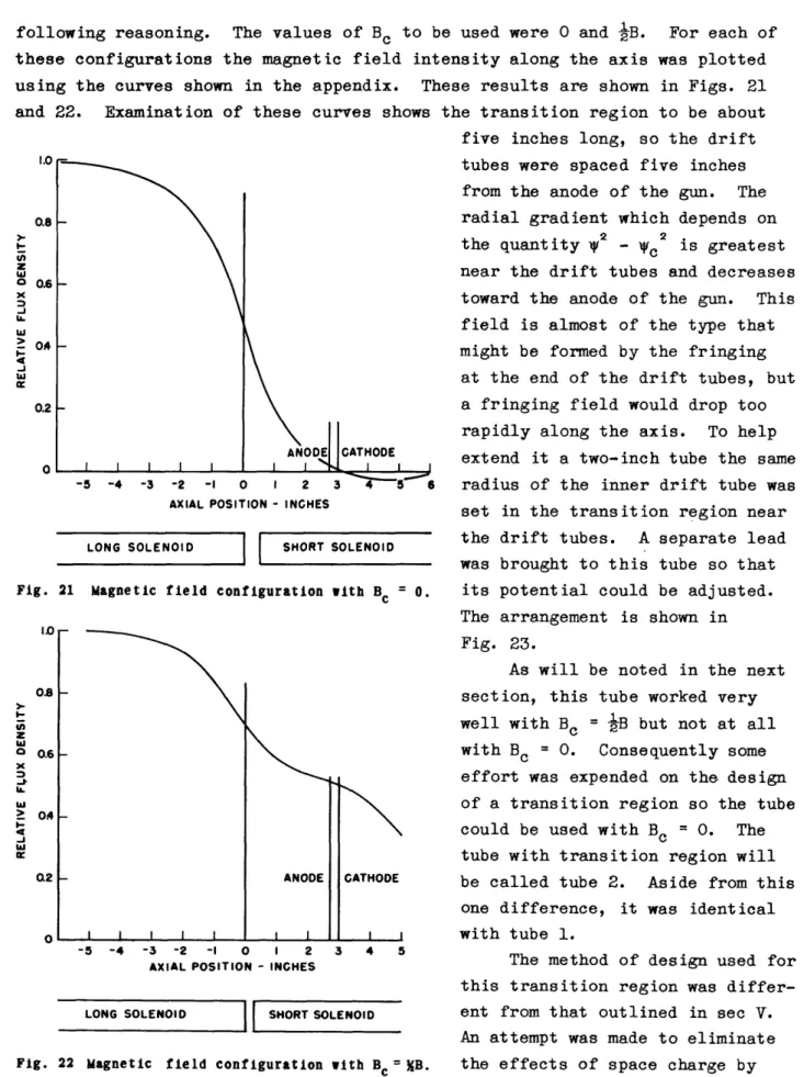
the method outlined above to something more practical by projecting the sur-face onto a plane and representing it as a family of curves. One possible projection is shown in Figs. 9 and 10 where a is chosen as parameter. The

600

LIMIT OF REAL VALUES

500- a= 100

-J 400 \a800

. 300 DESIGN CHART FOR a600

_o > a POSITIVE 200 e a400 I100~ W22 aO200 100 ~ / /'...a=1o 0 I I I 1HiI i I '-- lllil 1ll ' l"l ~ l 106 105 I4 10-3 02 10- ' 10 -K MKS UNITS

Fig. 9 Equation 78 with positive.

U60 500 En J 400 o 0 300 200 100 0 160 105 104 102 102 10 1 10 -K MKS UNITS

Fig. 10 Equation 78 with a negative.

projection of the design prism is a rectangle which is moved around on the design chart (Figs. 9 and 10) until the appropriate corners fall on two con-stant a curves which differ by the proper amount. As before, the resulting values of a, -K, and y - V may be read for either of the corners and the

-24-a=

-10iOOv-DESIGN CHART FOR a =-800v

_- a NEGATIVE

e

/a=-800v--- K r /

-400v-- /// Illi~l I I a = - 200v-i

-2OOv-corresponding voltages and magnetic field determined from these.

In some cases it may happen that we do not have complete freedom in plac-ing the rectangle where it will fit exactly as required. When this occurs, we must be careful to choose a position such that any error in y - V is an excess over the optimum value. If y is smaller than the value needed to give zero oscillation at any particular radius, the electrons in that shell do not have enough energy to have the prescribed values of z and r. As the angular ve-locity is fixed by the magnetic field, the axial veve-locity will be too low, or the electrons will never get to the point in question. Figure 11 shows the

correct metnoa or placing tne rec-tangle when it cannot be fitted to the curves ideally.

If the rectangle is set so high that neither corner lies on the

ap-CORRECT INCORRECT propriate a curve, tne entire beam

CORRECT INCORRECT

must oscillate and our purpose of Fig. 11 Methods of placing the design rec- minimizing the oscillation is not

tangle on the chart. achieved. In general then, we shall

always set at least one corner of the rectangle on the appropriate curve. The question of which a curve is the appropriate one is settled by the choice of the end of the diagonal used to read off the final parameter values. Thus for any particular setting the parameters are read from the end that will make the other point err by an excess in y. For example, on the right side of Fig. 11,

instead of reading the parameter values from the point a as indicated, they should be read from the point b. Then the curve corresponding to the value of a at ra will lie below a, as shown on the left.

This mention of errors in the design procedure leads us to consider their evaluation. This is obtained quite simply from the design chart. If the error in y - V is denoted by 6, as indicated in Fig. 11, then the actual value of y - V is given by

- V = (y - V)opt. + . (86)

Substituting (86) into (77) we obtain

2 -2K( - V) opt. - (l+K - 1)2 2K6

2 + Ka 2 + Ka (87)

The first term of (87) is zero by definition of (y - V)opt. and we are left with

2 -2K6

x = ₍₈₈₎

2 + Ka

by means of Fig. 4 or Eq. 42.

Once a location for the rectangle on the design chart is chosen we are left with the evaluation of the actual voltages to be applied to the electrodes and the magnetic field to be used; i.e. with the evaluation of T,, 2 and B.

The magnetic field is given directly by the chosen value of K. It is more convenient to use the representative point for the inside edge of the beam than any other. By definition

e/m Ka 2 2 WH ra and e B WH = m 2 Therefore 2 B (89) ra e/m (89)

The potentials are calculated from the equations developed in sec. III. At r = r_a the integrals in (66) become zero and we have

ra + (90) Pa = Ya = a in + 1(90) rl and r 1 = Ya - a n . (91)

The value of a is given by Eq. 79

a = a Consequently r 91= Ya - a In (92) rl and TP2 (Pi = La ln _r - _2nE - n _rb + _{e n (n+} n ₂₎₂ )2 _(rrn+ 2 ran + 2) b Pn n+ 2 n rb nO n+ 2 ra ] (93)

Equations (89), (92), and (93) are used after the parameters a, Ya, and K_a are chosen from the design chart.

The procedure outlined in this section is general in that it may be ap-plied to a beam with an arbitrary radial charge distribution and no restriction has been placed on the problem other than those enumerated earlier. The design

-chart is somewhat unwieldy because of this general character. In many cases the shape of the magnetic field in and near the cathode region is limited to certain special configurations. These limitations control the possible charge distributions in the beam. It is this practical restriction imposed by the magnetic field which narrows our field of inquiry to a few special cases where the design procedure can be carried out without the use of the chart. Instead, Eq. 78 is used directly to find the proper values of a', a, and Ka, and then

(89), (92), and (93) are applied to complete the design of this section of the beam system.

The next section, in which we examine the end conditions shows how these special cases arise.

V. END CONDITIONS: INJECTION OF THE BEAM

Up to this point we have considered only one part of the problem of pro-ducing electron beams in a magnetic focusing field. We have learned how a beam, once in a uniform magnetic field, will behave, and what voltages and

magnetic field strength are necessary for equilibrium. This behavior that has been analyzed is only one particular type or "mode" out of many possible ones. It

is certainly possible, for example, to have a beam in equilibrium in which the axial velocity differs from shell to shell. In this section we take up the problem of finding means to bring about the particular type of operation that we want.

It is necessary to consider the following questions: How do we get the required current into the beam? How do we insure that all electrons will have the same axial velocity? How do we get the beam into the desired re-gion (between ra and rb) so that it will stay there according to the analysis?

The answers to these questions proposed in this section are not intended to be general. Only one particular method of solving these problems is sug-gested, and it is to be emphasized that there are other and possibly more

fruitful lines of attack which could have been followed. The particular viewpoint taken here was chosen because of relative simplicity.

The foregoing remarks should be borne in mind as they are the basis for many of the restrictions and assumptions to follow. The results of the limited

analysis presented here will appear to be overly restrictive, but they are sufficiently flexible to allow for the discussion of a number of special cases

to be presented in the next section.

The functions of the end region of the beam system are such that it is expedient to break it up into two distinct sections, the electron gun and the transition region. Each of these parts will be considered separately and the

-27-functions of each will make the reason for the division evident.

The Electron Gun

The electron gun has its main use in supplying and controlling the beam current. It is not necessarily a function of the gun to accelerate the beam to the proper axial velocity or to any other particular velocity, but we shall assign this function to it. There are other requirements on the elec-tron gun, imposed by the ultimate uses of these systems, specifically their application in microwave tubes.

In microwave tubes, as in most other devices, it is desirable to reduce the noise to a minimum. This is one of the principal reasons for this en-tire study, since an efficient transmission of the beam through the drift tubes means a small contribution to the tube noise from partition of the beam current. The beam itself should be relatively free of noise fluctuations pro-duced by either shot effect or partition. To reduce the shot noise due to

initial velocities of emission, the cathode must operate in the space-charge limited regime, and to reduce partition noise, interception of the beam by electrodes should be small. The Pierce type of electron gun satisfies both of these demands as it has a high transmission efficiency and is space-charge limited. It is the only kind of electron gun capable of supplying the high current densities required in these systems.

The Pierce gun is well described in the literature and needs no further comment here (refs. 14 and 15). Design procedures for Pierce guns are avail-able only for certain cases in which the electron flow inside the gun itself

is rectilinear. The design, moreover, does not include the effects of mag-netic fields so that if we are to use available methods of gun design, we shall have to nullify the effect of the magnetic field.

It might be argued that if the magnetic field is to have no effect at the gun, then there should be no magnetic field, but this is not generally possible. If focusing is to be obtained, electrons must cross magnetic field lines and thereby acquire an angular velocity. Except for one special case, W. must be some nonzero quantity, and it is always different from the flux v linked by the electron shell in the uniform part of the beam.

Of course, we can still retain a finite value of *c and have no magnetic field in the gun region if we shield it. This procedure prevents magnetic flux from affecting the electron flow in the gun by guiding part of it through a central pole piece linking the cathode, and the remainder outside of the cathode as shown in Fig. 12.

In this configuration c is the same for all electrons regardless of the

position from which they originated at the cathode. The electron gun associated with such pole pieces operates independently of the magnetic field if the

shielding is good enough.

Another way of nullifying the effect of the magnetic field in the gun is to have it parallel to the lines of electron flow that would exist even without the field. If this condition is obtained the field cannot affect the beam since W

and yc are the same for any individual electron so long as it remains in the gun. The angular velocity is zero and the conditions assumed in designing the gun hold true.

This alternative configuration insures that the

-- - ng-la An 4- 4n:+ r no +A- +k -A

-uidulltJ.L; 1 I 1l-LU LU. Iu llU1 C1- a V LtLAL Lby J. LUt Ci -a UOU

Fig. 12 A magnetically is normal to it. The significance of the fact is

con-shielded electron gun. siderably greater than that it allows us to design the

gun. It means that we can be reasonably sure that thermal velocities of emission have negligible influence on the problem and that the noise will not be excessive.

Suppose there were a magnetic field oblique to the cathode surface in its immediate vicinity. The component of field parallel to the cathode surface where the electron velocities are low bends the trajectories around and builds

up a high space-charge density which suppresses any further emission. This situation is analogous to that in the cut-off magnetron. In order to get a true picture of the potential and space-charge distribution in this case, we should have to take into account the thermal velocities of emission. Twiss

(ref. 16) has considered this problem and has shown that neglect of thermal velocities in these cases can lead to serious error. Where the field is parallel to the electron paths and normal to the cathode, the Pierce gun should operate almost as though there were no magnetic field, and experience has shown that in this case thermal velocities introduce little error. Tiss has also shown that a large part of the preoscillation noise in the magnetron arises from the situation just discussed. The relative motions of the various streams of electrons moving out from the cathode and back towards it produces space-charge amplification of the noise already present. This mechanism is absent to a large extent in the system proposed here where the magnetic field

is purely normal to the cathode surface.

It was mentioned earlier that we would assign to the gun the function of accelerating the beam to some particular voltage. The main reason for this

is to get the electrons to a high enough velocity before they start to cross field lines. If this is not true, we get into the same trouble as we would

-29-if we had the transverse field near the cathode. With a previous acceleration the effect of the transverse field is, to a high degree of accuracy, the same for all electrons, having a common c so that we can be quite sure there is no serious error due to the thermal velocity distribution.

The Transition Region

The role of the transition region should now be apparent. It is in this part of the system that the beam crosses magnetic field lines and acquires the angular velocity it needs for focusing in the useful part of the system. The electron trajectories at the two extremes of this region are specified; at the gun anode all electrons have essentially the same axial velocity, and at the beginning of the uniform field, all electrons must have a common specified axial velocity, the proper angular velocity and no radial velocity. Our prob-lem now is to find a trajectory in the transition region that links the gun and the uniform field sections and has the properties just mentioned at either of its ends.

It is not possible to solve for this trajectory unless the geometry and potentials of the system are entirely specified, but it is our object to find the geometry and required potentials in the transition space. Finding the electron path from a set of known conditions where the magnetic field is non-uniform is an extremely difficult task. It would involve a repetition of the analysis of sec. II where the z independence is lost. The alternative is to specify a trajectory with the necessary characteristics and then to find the geometry and potentials consistent with the assumed electron motion.

The simplest path we can assume is a constant radius one. This results in a system having the general

'BEAM

j

I

GUN TRANSITION UNIFORM FIELD

Fig. 13 Constant radius beam

system.

form of that shown in Fig. 13 where the elec-tron beam maintains its shape all the way from the anode of the gun through the uniform part

of the system where it is put to use. The constant radius path clearly satisfies the

con-ditions necessary at the gun anode and at the entrance to the drift tubes. The problem to be solved now is to find the conditions which cor-respond to the assumed path and how to satisfy these conditions by shaping the electrodes as indicated in Fig. 13.

The magnetic field configuration is assumed to be known everywhere, so we have to find the electric potentials and fields that, in combination with

the magnetic field, will keep the electrons on their specified paths. We