Bayesian Level Sets and Texture Models for Image
Segmentation and Classification with Application
ARGH
ARSCHUS NE
to Non-Invasive Stem Cell Monitoring
S-7OF TECHNOLOGYby
Nathan Christopher Lowry
JUL 19 2013
B.S.M.E., Rice University (2001)
M.S.M.E., Rice University (2004)
LIBRARIES
Submitted to the Department of Aeronautics and Astronautics
in partial fulfillment of the requirements for the degree of
Doctor of Science in Aeronautics and Astronautics
at the
MASSACHUSETTS INSTITUTE OF TECHNOLOGY
June 2013
@
Nathan Christopher Lowry, MMXIII. All rights reserved.
The author hereby grants to MIT permission to reproduce and to
distribute publicly paper and electronic copies of this thesis document
in whole or in part in any medium now known or hereafter created.
, r Z'7
A uthor
.. .
. ...
Department of Aeronautics and Astronautics
11
-l1,
2013
Certified by...
C
i Ui-
1-Youssef M. Marzouk
Class of 1942 Associate Professor, MIT
Thesis Supervisor
e y...
--- R&1~5Tiangoubi
Principal Member of the Technical Staff, C.S. Draper Laboratory
/
I
A
,Thesis Supervisor
Accepted
by..
...
Eytan H. Modiano
Profesor of Aeronautics and Astronautics, MIT
Chair, Graduate Program Committee
Thesis Committee Members
Youssef M. Marzouk, Ph.D. Class of 1942 Associate Professor Massachusetts Institute of Technology Rami S. Mangoubi, Ph.D.
Principal Member of the Technical Staff
C.S. Draper Laboratory
Laurent Demanet, Ph.D.
Assistant Professor of Applied Mathematics Massachusetts Institute of Technology Mukund N. Desai, Ph.D.
Distinguished Member of the Technical Staff
C.S. Draper Laboratory
Paul J. Sammak, Ph.D. Scientific Review Officer National Institute of Health
Bayesian Level Sets and Texture Models for Image
Segmentation and Classification with Application to
Non-Invasive Stem Cell Monitoring
by
Nathan Christopher Lowry
Submitted to the Department of Aeronautics and Astronautics on May 10, 2013, in partial fulfillment of the
requirements for the degree of
Doctor of Science in Aeronautics and Astronautics
Abstract
Image segmentation and classification, the identification and demarcation of regions of interest within an image, is necessary prior to subsequent information extrac-tion, analysis, and inference. Many available segmentation algorithms require man-ual delineation of initial conditions to achieve acceptable performance, even in cases with high signal to noise and interference ratio that do not necessitate restora-tion. This weakness impedes application of image analysis to many important fields, such as automated, mass scale cultivation and non-invasive, non-destructive high-throughput analysis, monitoring, and screening of pluripotent and differentiated stem cells, whether human embryonic (hESC), induced pluripotent (iPSC), or animal.
Motivated by this and other applications, the Bayesian Level Set (BLS) algorithm is developed for automated segmentation and classification that computes smooth, regular segmenting contours in a manner similar to level sets while possessing a sim-ple, probabilistic implementation similar to that of the finite mixture model EM. The BLS is subsequently extended to harness the power of image texture methods by in-corporating learned sets of class-specific textural primitives, known as textons, within a three-stage Markov model. The resulting algorithm accurately and automatically classifies and segments images of pluripotent hESC and trophectoderm colonies with
97% and 91% accuracy for high-content screening applications and requires no
pre-vious human initialization. While no prior knowledge of colony class is assumed, the framework allows for its incorporation. The BLS is also validated on other applica-tions, including brain MRI, retinal lesions, and wildlife images.
Thesis Supervisor: Youssef M. Marzouk Title: Class of 1942 Associate Professor, MIT
Thesis Supervisor: Rami S. Mangoubi
:T
X
L1I(DV
Then Samuel took a stone, and set it between Mizpeh and Shen, and called the name of it Ebenezer, saying, Hitherto hath the LORD helped us.
Acknowledgments
I am most fortunate to have an incredible thesis advisor at Draper, Dr. Rami Man-goubi. Rami believed I had potential when we worked together on an industry project and graciously invited me to become his student as he began the leadership of his stem cell image analysis RO1 grant. Since then, he has been a keen mentor and strong ad-vocate for my studies and research. This thesis would not have been written without his guidance, and I feel fortunate for the opportunity to continue collaborating with him after the conclusion of graduate study. Rami's insistence that research originates in real problems and requires new methods speaks to his high standards.
In addition, I would like to thank my advisor at MIT, Prof. Youssef Marzouk, who graciously agreed to advise a student researching image processing. His cheerful
and patient guidance was invaluable in navigating MIT.
Thank you to Dr. Mukund Desai, not only for serving on my thesis committee but for the many conversations and brainstorming sessions. The texture content of this thesis has particularly benefited from his insight.
Thank you to Dr. Paul Sammak, who not only provided high-quality image data for analysis but patiently and clearly explained stem cell biology to engineers. The biological application of my research was motivated by the knowledge Paul imparted and his advocacy of image-based biomarkers.
Thank you to Prof. Laurent Demanet for serving on my thesis committee, and to Dr. John Irvine for acting as a reader. My special thanks to Dr. Michael Prange for acting as an emergency reader and Dr. Tarek Habashy for introducing us. I appreciate very much the time and helpful comments you have all provided.
Thank you also to Prof. Gustavo Rohde, who graciously reviewed my defense the night before its delivery. The presentation (and my confidence in giving it) were stronger for his comments.
Thank you to Dr. Igor Linkov and Prof. Matteo Convertino for inviting me to collaborate on their biodiversity research. And thanks also to Dr. Alexander Tkachuk, for introducing us and for many stimulating conversations on decision theory.
I owe thanks to a great many people at Draper Laboratory. I particularly thank
Linda Fuhrman, Steve Kolitz, and Sharon Donald for generously supporting my
the-sis; the laboratory is fortunate to have officers who value the development of research
skills. Thanks to Pam Toomey, an artist with a gift for designing conference posters
which are both informative and aesthetically appealing. Many thanks also to Heidi
Perry. I have often heard from Rami how she values good researchers, and I am
grate-ful that, after I expressed an interest in continuing at Draper Laboratory following
my studies, she acted with alacrity to ensure that I would be rehired. Thanks also
to Dr. Leena Singh for her interest in my research and to Dr. Piero Miotto, whose
advice and recommendation at the beginning of my studies was especially helpful.
Thank you to all my friends for your support. I particularly thank Matt Agen,
Josh Ketterman, and Nick Mulherin, for conversation, games, and good humor. And,
I specially thank Rob Rodger, an old and true friend who recently gave up a weekend
to sit by a table in the woods so that I might be engaged.
Thank you also to my future in-laws, the Gabrielse family, who have welcomed
me into their family and kindly attended my defense in support.
I am very, very grateful for the steadfast love and support my family has given
me during my years in graduate school. Thank you to my parents, Dr. J. Michael
and Jolynn Lowry, and to my sister Sarah, her husband Steven Meek, and their new
daughter Grace. Your words of encouragement during pre-quals jitters, in the midst
of late-night coding sessions, and this final year of research and writing were a very
real source of strength.
And, finally, I would like to thank my wonderful fiancee, Abigail Gabrielse. I
resolved to ask her out to dinner the very day I submitted my thesis proposal and
proposed to her three weeks prior to my defense. In her kindness and love, she served
as the first proof reader for this document and sent many a home-cooked meal with
me to the lab. To me she has been a great encouragement and a great joy, and I feel
incredibly blessed that we are to be married. Many women do noble things, but you
surpass them all. Abigail, sans toi,
a
qui sourire? Pour qui vivre?
Assignment
Draper Laboratory Report Number T-1744
In consideration for the research opportunity and permission to prepare my thesis by and at The Charles Stark Draper Laboratory, Inc., I hereby assign my copyright of the thesis to The Charles Stark Draper Laboratory, Inc., Cambridge, Massachusetts.
a n Lowry Date
2dr3
This thesis was prepared at The Charles Stark Draper Laboratory, Inc., with sup-port by NIH grant 1 R01 EB006161-01 and by an internal research and development grant from Draper Laboratory.
Publication of this thesis does not constitute approval by Draper or the sponsoring agency of the findings or conclusions contained herein. It is published for the exchange and stimulation of ideas.
Contents
1 Introduction
23
1.1 Need for automated segmentation and classification . . . . 24
1.2 Need for non-invasive biomarkers for stem cell monitoring . . . . 26
1.2.1 Importance of stem cells . . . . 26
1.2.2 Current practices . . . . 28
1.2.3 Image analysis as a non-invasive, non-destructive stem cell biomarker 29 1.3 C ontributions . . . . 29
1.3.1 Contributions to image segmentation and texture modeling . . 30
1.3.2 Contributions to non-invasive, quantitative, image-based stem cell biom arkers . . . . 32
1.4 O rganization . . . . 32
2 Level Sets and Expectation-Maximization: A Comparative Analysis 35
2.1 Notation and conventions . . . . 362.2 Level sets . . . . 38
2.2.1 History of level sets . . . . 38
2.2.2 Region-based level sets . . . . 40
2.2.3 Further development . . . . 44
2.3 Expectation Maximization (EM) of finite mixture models . . . . 45
2.3.1 Development and theory . . . . 46
2.3.2 Finite mixture model EM .. . . . . 47
2.3.3 Use in image segmentation . . . . 49
2.5
Conclusions and commentary . . . .
3 Bayesian Level Sets for Image Segmentation
3.1
Formulating the cost function . . . .
3.1.1
The cost function . . . .
3.1.2
Interpretation and insight . . . .
3.2
A Bayesian identity for minimizing the cost function
. . . .
3.3
A Bayesian level set algorithm for multiclass image segmentation . . .
3.4 Geometric and smoothing priors . . . .
3.5
Advantages of the BLS . . . .
3.6
The BLS and the EM . . . .
3.7 Example applications of the BLS . . . .
3.7.1
A simple example . . . .
3.7.2
Wavelet texture-based segmentation of induced pluripotent stem
cells . . . .
3.7.3
Noisy brain MRI . . . .
3.7.4
Massively multiclass segmentation of stem cell nuclei via hard
classification . . . .
3.8 Sum m ary . . . .
The Power of Texture for Image Classification
4.1
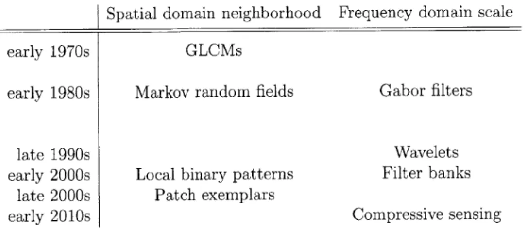
Historical review of image texture modeling . . . .
4.1.1
Spatial domain neighborhood models . . . .
4.1.2
Frequency domain scale models . . . .
4.2 Wavelet-based texture classification of stem cell patches . .
4.2.1
Wavelet-based texture analysis . . . .
4.2.2
Application to nuclei classification . . . .
4.2.3
Application to colony classification via windowing .
4.3 Texture features for stem cell colony segmentation . . . . .
4.3.1
Localizing texture models for image segmentation
4.3.2
Wavelet-based features (dcmag, dcmax, and wave)
51
55
55
56
57
59
61
65
68
70
71
71
73
77
79
83
485
. . . .
86
. . . .
88
. . . .
90
. . . .
91
. . . .
92
. . . .
96
. . . .
100
. . . .
104
. . . .
104
. . . .
106
4.3.3 Other filter-based features (abar, gauss, log) . . . . 4.3.4 Entropy-based features (hdiff, hloc) . . . .
4.3.5 Compressive sensing features (cs) . . . .
4.3.6 Comparative summary . . . .
4.4 Sum m ary . . . .
5 Texture-based Segmentation using Bayesian Level Sets
5.1 The texture-based Bayesian Level Set algorithm . . . . 5.1.1 Three-stage Markov texture model . . . .
5.1.2 Adapting the three-stage Markov model in the BLS framework
5.1.3 Geometric prior: combine smoothing and mixture . . . .
5.1.4 Conjugate data priors: Normal-inverse-Wishart and Dirichlet .
5.1.5 The texture-based Bayesian Level Set algorithm . . . .
5.2 T raining . . . .
5.2.1 Feature selection . . . .
5.2.2 Feature reduction via Principle Component Analysis (PCA) .
5.2.3 Texton learning via GMM-EM clustering . . . .
5.3
5.4
5.5
Initialization . . . . Case Study: Zebras . . . .
Summary ... ...
6 Texture-Based BLS Applied to Non-Invasive Stem
mentation and Classification
6.1 Motivation and impact . . . .
6.2 Virtual staining . . . .
6.3
Data collection . . . .
6.4 Colony image segmentation . . . .
6.4.1 Experimental procedure . . . .
6.4.2 Numerical results . . . .
6.4.3 Evolution of a single BLS segmentation . . .
6.4.4 Texton training for differentiated colonies . .
Cell Colony Seg-143 . . . . 143 . . . . 145 . . . . 145 . . . . 145 . . . . 146 . . . . 146 . . . . 149 . . . . 149 108 110 112 113 115
117
117 118 122 123 125 129130
132 136 139 139 141 1426.5
Multi-class image phantom segmentation . . . .
161
6.6 Recognizing anomalous texture classes . . . .
163
6.7 Conclusions . . . .
164
7 Summary, Contributions, and Suggestions for Future Work
165
7.1
Contributions . . . .
165
7.2
Suggestions for future work . . . .
167
A Notation
169
B Derivations for smoothing conditions
171
B.1 Diffusion from energy . . . .
171
B.2 Curvature from total variation . . . .
172
B.3 Curvature from contour length . . . .
173
C Derivation of the GMM-EM
175
C.1 Derivation of the GMM-EM update equations . . . .
175
C.1.1 Expectation step . . . .
176
C.1.2 Maximization step . . . .
176
C.2 Derivation with Dirichlet and Normal-Inverse Wishart priors . . . . .
177
C.3 Derivation of the three-stage GMM-EM . . . .
179
C.3.1
Expectation step . . . .
180
List of Figures
1-1 Image segmentation defined. . . . . 25
1-2 Current state of the art in stem cell quality assessment. . . . . 27
1-3 A vision for automated human embryonic stem cell (hESC) cultivation. 28
1-4 Stem cell colony segmentation. . . . . 30
2-1 Demonstration of level set segmentation. . . . . 40 2-2 Two-stage finite mixture model. . . . . 47
2-3 Smoothing prevents topological fracture in the segmentation of noisy im ages. . . . . 51 3-1 A simple example demonstrating the rapid convergence of the
multi-class B L S. . . . . 72
3-2 BLS segmentation of iPSC colonies using automated initial conditions. 74
3-3 Comparison of smoothing priors for BLS segmentation. . . . . 76
3-4 Retinal lesion segmentation. . . . . 77 3-5 Comparison of BLS and FMM-EM for MRI phantom segmentation. . 78 3-6 Noise analysis for BLS and FMM-EM for MRI phantom segmentation. 80 3-7 Massively multiclass BLS segmentation of fixed, early differentiating
cells. . . . . 8 1
4-1 Image texture as statistical fluctuation in image gray scale intensity. . 87
4-2 The generalized Gaussian distribution. . . . . 93
4-3 Nuclei classification via wavelet texture modeling. . . . . 97
4-5 Adaptive windowing for classification of small, irregularly shaped regions. 99
4-6 Window-based stem cell colony classification using wavelet texture
m odels.
. . . .
101
4-7 Impulse response of DWT and DT-CWT filters. . . . .
107
4-8 The filters for abaro and hdiffo-. . . . .
109
4-9 Texture feature comparison. . . . .
114
5-1
Three stage Markov texture model . . . .
118
5-2 A zebra's stripes are an example of texture. . . . .
119
5-3 A demonstration of the Markov texture model . . . .
120
5-4 In texture-based segmentation, the most likely texton varies within the
class. . . . .
12 1
5-5 The mixture prior suppresses outlier classes to prevent misclassification. 125
5-6 Data priors prevent misclassification due to overtraining. . . . .
126
5-7 Pluripotent and differentiated training images. . . . .
131
5-8 Mutual information-guided feature selection. . . . .
133
5-9 The hdiff texture feature is critical for successful segmentation near
colony boundaries. . . . .
133
5-10 dcmax is generally the most informative wavelet texture feature. . .
.
134
5-11 Segmentation precision limits neighborhood scale. . . . .
135
5-12 The predictive power of individual compressive sensing texture features
is low . . . .
136
5-13 PCA feature reduction. . . . .
137
5-14 Data reduced via PCA. . . . .
138
5-15 Pluripotent textons derived via the GMM-EM. . . . .
140
5-16 Zebra image segmentation using the texture-based BLS . . . .
141
6-1 Pluripotent colony segmentation accuracy. . . . .
147
6-2 Differentiated colony segmentation accuracy. . . . .
148
6-4 Simultaneous segmentation and classification of pluripotent stem cell
colonies (D -L). . . . . 151
6-5 Simultaneous segmentation and classification of pluripotent stem cell
colonies (M -U ). . . . . 152
6-6 Simultaneous segmentation and classification of pluripotent stem cell
colonies (V -BB). . . . . 153
6-7 Simultaneous segmentation and classification of differentiated stem cell
colonies (D -L). . . . . 154
6-8 Simultaneous segmentation and classification of differentiated stem cell
colonies (M -S). . . . . 155
6-9 Evolution of a single BLS segmentation: pluripotent colony
segmenta-tion label m ap. . . . . 156 6-10 Evolution of a single BLS segmentation: pluripotent colony geometric
p rior. . . . . 157 6-11 Evolution of a single BLS segmentation: pluripotent textons in feature
dim ensions 1 and 2. . . . . 158 6-12 Differentiated colonies inappropriate for segmentation via texture-based
B LS (T -W ). . . . . 159
6-13 Retraining differentiated texton priors to recognize diffuse colonies. . 160
6-14 Segmentation of mixed-class stem cell colony phantoms. . . . . 162
List of Tables
2.1 Comparative advantages of Level Sets and the FMM-EM. . . . . 53
3.1 Pseudocode for the Bayesian Level Set (BLS) algorithm. . . . . 62
3.2 Comparative advantages of Level Sets, the FMM-EM, and the BLS. . 68
4.1 The history of image texture modeling. . . . . 89
5.1 Pseudocode for a texture-based BLS algorithm. . . . . 129
6.1 Numerical results for simultaneous segmentation and classification of
Chapter 1
Introduction
The primary objective of this thesis is the formulation of an algorithm for automated simultaneous image segmentation and classification. The first algorithm proposed is the general purpose Bayesian Level Set (BLS), which produces smooth, regular borders just as level sets do and yet possesses a simple, probabilistic implementa-tion similar to that of finite mixture model Expectaimplementa-tion-Maximizaimplementa-tion. The second algorithm harnesses the power of image texture modeling for segmentation by in-corporating learned sets of class-specific textural primitives within the BLS via a three-stage Markov process. Early versions of the former and latter algorithms are seen in [63] and
[641.
The texture-based BLS is then applied to successfully automate the segmentation and classification of a set of unknown pluripotent and differenti-ated stem cell colony images with accuracy 97% and 91%, respectively, effectively demonstrating that this approach serves as a non-invasive, non-destructive,automat-able, statistical biomarker for stem cell classification and quality assessment that may
serve as a surrogate to microscopy or chemical staining [72, 102]. These two algo-rithms are also validated on other applications, including brain MRI phantoms, stem cell nuclei, and wildlife images.
1.1
Need for automated segmentation and
classi-fication
Image segmentation is the process of automatically dividing an image into its
consti-tutive disjoint regions, such as distinguishing the zebra in the foreground of the image in Figure 1-1 from the plain comprising the image background. As each region may be considered a separate class, image segmentation is essentially a labeling problem that assigns to each pixel or coordinate within an image a label based on the dis-tinct region to which it belongs. Segmentation is thus a necessary prelude to many other image analysis applications, including biomedical ones. For instance, in image-based high-throughput screening, segmentation might automatically demarcate a cell colony from its growth medium prior to analyzing or grading colony quality according to criteria such as image texture or shape. Likewise, in brain Magnetic Resonance Imaging (MRI) classification, brain tissues are first segmented as a preliminary step before identifying or classifying tumors or diseased tissue. Non-medical applications might include biome identification in satellite imaging [24] or video motion tracking or surveillance, in which the same object must be located and accurately segmented across a time series of video frames. As the applications of segmentation are rich and varied, a wide variety of segmentation algorithms exist, including thresholding [84],
region growing [44], Expectation-Maximization [59, 60], phase fields [52, 91], graph cuts [9, 10], level sets [18, 115], etc.
While these algorithms vary, most attempt to balance the image data and region geometry in determining a final segmentation. Image data quantifies the variation in local appearance between regions. In the absence of geometric criteria, however, purely data-driven approaches often result in the misclassification of pixels due to noise and outliers. Consideration of region geometry accounts for the observation that, within the human field of vision, the location of an object is grouped in one region of space and its perceptual interface with its background is generally smooth or rounded. Some approaches, including most Markov random field and graph cut algorithms, address this consideration by inducing pairwise dependence between the
(a) Zebra Image (b) The Image Segmented (c) Label Map
Figure 1-1: Image segmentation defined. (a) A zebra (foreground) standing on a plain (background);
(b) a segmentation of this image using the algorithm in section 5.4, the red segmenting contour
de-marcates the zebra from the image background; (c) the label map corresponding to this segmentation, label 1 (blue) identifies a pixel as belonging to the image background while label 2 (red) indicates the zebra. Note that the shadow below the zebra, which is very similar in intensity and shape to the zebra's stripes, is correctly segmented.
classification of a pixel and its immediate neighbors. Level set algorithms attain even smoother results over larger neighborhoods by penalizing the curvature of the segmenting contour. While these techniques may be powerful. they are generally far more difficult to implement than algorithms such as Expectation-Maximization, which typically either forgoes geometric criteria or is limited to static prior atlases.1
A simpler and more computationally efficient approach to implementing geometric
criteria in segmentation is needed.
A further complication is the tight connection between segmentation and another
problem often performed separately in image processing literature: classification, recognizing the identified region and assigning it to a class based on a library of prior examples. Together, segmentation and classification constitute a chicken-and-egg type
problem for many non-trivial images. If the classes are stipulated (e.g. pluripotent
cells and growth media in a cell colony image), it would be possible to segment an image according to the characteristics indicative of those classes. Likewise, the statistics of regions in a segmented image would enable classification. Performing these tasks simultaneously, however, is often quite challenging.
This thesis builds upon and extends insights from prior approaches to formu-late a segmentation and classification algorithm that fuses the powerful geometric
1
A segmentation atlas assigns a prior probability to each class at each pixel and is commonly
used for problems in which the general shape of solution is known, such as brain MRI segmentation or object recognition.
criteria of level sets to a simple, probabilistic implementation similar to
Expectation-Maximization. The resulting Bayesian Level Set (BLS) returns segmentations with
smooth, regular borders, natively extends to multiple image regions, and optionally incorporates data priors in order to simultaneously segment and classify images.
1.2
Need for non-invasive biomarkers for stem cell
monitoring
The motivating application for the development of the BLS is automating the seg-mentation and classification of stem cell colony images. While stem cells offer many exciting possibilities for therapeutic and research use, one of the key bottlenecks in de-veloping this technology is the lack of a procedure for automated stem cell cultivation. Current state-of-the-art in stem cell monitoring requires either manual inspection by a trained microscopist, which is costly, time consuming, and necessarily subjective, or chemical staining, which is destructive and renders a colony unfit for further use. This alternatives are illustrated in Figure 1-2. Image processing offers the possibility of a non-invasive, non-destructive, statistical biomarker for stem cell quality assessment and monitoring, which may potentially serve as an enabling technology for automated stem cell cultivation as in Figure 1-3.
1.2.1
Importance of stem cells
Due to their pluripotency and longevity, pluripotent stem cells have been of intense interest to biomedical researchers in the fifteen years since the 1998 discovery of a practical procedure for the cultivation of human embryonic stem cells (hESC) by researchers under the direction of Dr. James Thomson at the University of Wisconsin-Madison [114]. Stem cell lines are capable of long-term self renewal and are effectively immortal when cultivated under laboratory conditions. More importantly, however, hESCs are pluripotent and have yet to specialize into any of the specific cell types that comprise the human body. By contrast, stem cells which have begun to specialize
(a) Chemical Staining (b) Microscopy
Figure 1-2: Current state of the art in stem cell quality assessment. (a) Chemical staining is rapid, automatable, and precise, but destructive and renders the colony unfit for further research or ther-apeutic use; (b) microscopy is non-invasive and non-destructive but non-quantitative and requires a trained microscopist to analyze results by eye.
to some degree are termed differentiated [79]. More recently, the 2006 discovery by Takahashi and Yamanaka of a procedure to create induced pluripotent stem cells (iPSC) [113] by effectively "de-differentiating" adult cells into a pluripotent state offers the potential to mitigate the ethical and political concerns surrounding the manufacture of pluripotent cells from human embryos.
The pluripotency of hESCs and iPSCs offers exciting possibilities to biomedical re-searchers. In addition to basic research in human embryology and early development,
potential therapeutic and research applications of stem cells include:
Tissue growth. The possibility for clinician-directed differentiation of stem cells
into specific types might allow for cell-based therapies in which tissues are produced in the laboratory and then transplanted into a human body to replace damaged or destroyed cells without triggering an immune response. Potential applications include Parkinson's disease [6], diabetes [67], and heart disease [129].
Drug discovery. Another possible near-term use of pluripotent stem cells is
high-throughput screening in drug research and discovery. In such procedures, mass testing is used to discover potential druggable compounds and assess their potency and side effects or toxicity by treating an array of diseased and healthy cells and tissues with a wide variety of test compounds. Again, directed differentiation of stem cells might
HTurEbryonic Ole Um Algorithm
Image Classification and Monitoring (CSDL/MWRI): Non4nvasive, Non-destructive, Continuous, Consistent, Automatable
Figure 1-3: A vision for automated human embryonic stem cell (hESC) cultivation. Cultures are robotically imaged and the results sent to sophisticated algorithms which assess the quality and state of the cultures via image texture methods. Based on this automated assessment, the colony's environmental conditions are adjusted, such as by the infusion of nutrients or growth factors, in order to maintain pluripotency, promote growth, or direct differentiation subject to the orders of a human supervisor [71, 102].
allow for precise mass production of the targeted cells and tissues [101].
1.2.2
Current practices
At present, there are an estimated twelve thousand stem cell colonies under labora-tory cultivation; therapeutic application of stem cell technology mandates increasing this quantity by at least an order of magnitude. A chief impediment to doing so is the current lack of an automatable, non-invasive, and non-destructive means of
mon-itoring, testing, and cultivating cell colonies as illustrated in Figure 1-3. Stem cells
are comparatively fragile, and differentiated cells tend to induce nearby pluripotent cells to differentiate. Therefore, each hESC or iPSC colony must be inspected every two days in order to remove damaged cells and pockets of spontaneous differentiation that might lead to a chain reaction causing the entire colony to differentiate [37, 85]. Unfortunately, neither of the two current state-of-the-art methods for stem cell inspection is suitable to mass cultivation. While biochemical and immunochemi-cal staining tests exist that are rapid, consistent, and automatable, results are non-quantitative and the applied chemical factors are destructive, killing the cells and
rendering them unsuitable for further research or clinical use. In practice, there-fore, researchers rely on visual inspection of stem colonies via brightfield microscopy, interpreting the state of the colony from its morphological properties. While this procedure is non-invasive and allows for further use of the colony, it is necessarily subjective and non-quantitative. More important, however, are the time and expense associated with training microscopists and having them manually inspect cell colonies. Simply put, there are not enough of these skilled individuals for them to check each of the many thousands of colonies necessary for widespread cultivation, and if there were, their time could be put to better use.
1.2.3
Image analysis as a non-invasive, non-destructive stem
cell biomarker
Image analysis presents a potential solution, if segmentation and classification meth-ods were developed to automate the inspection tasks now performed by microscopists. Automated mass screening of cell colonies might be enabled by algorithms sufficiently accurate to identify the type and approximate location and size of cell colonies and flag questionable or differentiating colonies for further analysis. The hardware infras-tructure for large scale, automated image collection of cell cultures already exists in many laboratories. Computer-based image processing is therefore a potentially en-abling technology for automated non-invasive, non-destructive monitoring of stem cell colony cultivation in a manner that is scalable and exceeds the rate of human-possible classification.
1.3
Contributions
The key contributions of this thesis fall into two major categories:
1. Image segmentation and texture modeling. This thesis introduces a Bayesian
Level Set (BLS) algorithm for image segmentation, which combines the advan-tages of two existing segmentation algorithms: level sets and the finite mixture
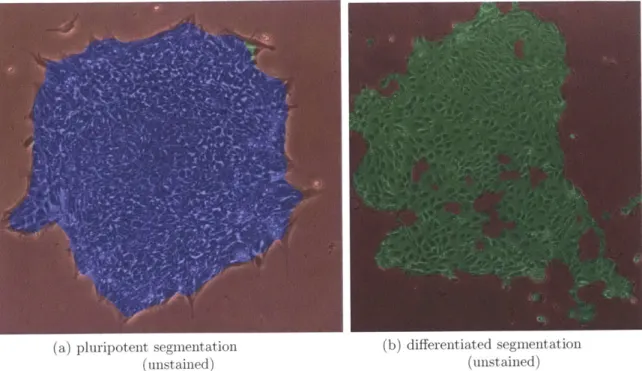
(a) pluripotent segmentation (b) differentiated segmentation
(unstained) (unstained)
Figure 1-4: Stem cell colony segmentation. pluripotent (a) and differentiated (b) colonies segmented and classified as in chapter 6: blue regions were classified pluripotent, green differentiated, and red media: image colorization was performed via computer and no chemical staining was applied to the colony.
model EM, and the development of texture methods for image classification.
2. Non-invasive, non-destructive image-based stem cell biomarkers. This thesis demonstrates that image texture constitutes a non-invasive, non-destructive biomarker for segmenting and classifying stem cell images, which may enable future automated stem cell monitoring and cultivation.
1.3.1
Contributions to image segmentation and texture
mod-eling
Major contributions
1. A new Bayesian Level Set (BLS) algorithm for image segmentation (chapter 3).
The key intuition underlying this iterative approach to segmentation is that a geometric smoothing prior computed from the a posteriori classification may be used to encourage local similarity in labeling, with the result that the BLS
produces the smooth, regular segmenting contours typical of level sets using a Bayesian approach akin to that employed by Finite Mixture Model
Expectation-Maximization (FMM-EM).
Compared to the FMM-EM, the geometric smoothing prior of the BLS:
" noticeably reduces misclassification due to outliers, and
" returns far more natural segmenting contours.
Compared to level sets, the BLS:
" is simpler in implementation, requiring neither the solution of partial
dif-ferential equations nor ancillary algorithms,
e natively extends to an arbitrary number of classes without complicated mathematical machinery, and
" requires far more lenient initial conditions, demonstrating a capture radius
which exceeds that typical of level sets.
Earlier versions of this algorithm were demonstrated in [63, 64].
2. Simultaneous segmentation and classification via a texture-based BLS (chapter
5). By incorporating image texture modeling into the BLS framework via a
three-stage Markov texture model, texture may be used to automatically iden-tify the types of regions within an image that may be then segmented via the BLS. This algorithm incorporates all the other advantages of the BLS and is used to automate the simultaneous segmentation and classification of a set of pluripotent and differentiated stem cell images as described in section 1.3.2.
Minor contributions
Traditional image texture models are of little use for segmentation as they depend on statistics calculated over rectangular, texturally homogeneous windows. For seg-mentation, texture features must be calculated at each coordinate, rather than over a fixed window, and must necessarily be modeled near the interface between the
textures to be segmented, precluding homogeneity. Extension of the BLS algorithm
to texture-based segmentation generated two minor contributions to image texture
modeling:
1. A framework for localizing image texture models for segmentation (section 4.3.1).
Texture feature dimensionality is reduced by retaining only the maximal
re-sponse over orientation at a particular scale. Localized statistics are then
com-puted by utilizing Gaussian smoothing to compute a weighted local average.
2. An adaptive windowing method for texture-based classification of small,
irregu-larly shaped image regions (section 4.2.2). Applications include cell nuclei [65].
1.3.2
Contributions to non-invasive, quantitative, image-based
stem cell biomarkers
By automating the simultaneous segmentation and classification of a series of
pluripo-tent and differentiated stem cell colony images, it is demonstrated that image texture
serves as a non-invasive, non-destructive biomarker for assessing stem cell
pluripo-tency status. This quantitative, statistical biomarker serves as a surrogate or
poten-tial replacement for destructive chemical staining that renders a colony unsuitable
for further use in cultivation, therapy, or research. By eliminating the need for direct
human observation of the majority of stem cell colonies, image texture-based
screen-ing offers the potential for quantitatively monitorscreen-ing stem cell quality at a greatly
increased spatial and temporal resolution relative to current practices in microscopy
or chemical staining. This contribution may eventually enable automated cultivation
of stem cells and their derivatives.
1.4
Organization
The organization of this thesis is as follows.
Chapter 2 describes the history of and introduces the mathematical background
(FMM-EM), the two prior segmentation algorithms most influential to the development of Bayesian level sets. After describing these algorithms and deriving their update equations from corresponding utility functions, the relative advantages and difficulties of the two approaches are assessed.
Chapter 3 formulates the basic Bayesian Level Set (BLS) algorithm. The BLS
is first formulated by demonstrating that the level set minimizing conditions may be reached via a Bayesian implementation similar to the FMM-EM by imposing a prior derived from curvature-based smoothing of the a posteriori classification. Subsequently, the similarity of the BLS to the EM is explored and various means are noted of extending and modifying the prior via geometric transformations of the
a posteriori classification. The advantages of the BLS with respect to convergence
rate, multi-region segmentation, and ease of initialization are then demonstrated on a variety of problems including basic segmentation of iPSC colonies, retinal lesions, MRI brain phantom images, and stem cell nuclei.
Chapter 4 introduces image texture and demonstrates its suitability for
classi-fying stem cell colony images. This chapter first summarizes the history of image texture methods, distinguishing between approaches which define textural neighbor-hoods in the spatial or frequency domains. It next shows that texturally homogeneous stem cell images may be classified very accurately using wavelet texture methods, a species of frequency-domain approach. Finally, it introduces a framework for localiz-ing image texture for use in segmentation and describes a variety of suitable texture models.
Chapter 5 incorporates the texture methods described in chapter 4 within the
BLS framework introduced in chapter 3 via a three-stage Markov texture model. After imposing data priors in order to allow for simultaneous segmentation and clas-sification, the chapter discusses the training of the algorithm via feature selection, reduction, and clustering with reference to the classification of stem cell colonies.
Chapter 6 demonstrates the application of this algorithm to the simultaneous
segmentation and classification of stem cell colonies. Pluripotent results are near perfect at 97% accuracy, and differentiated results are accurate to within 91%.
Chapter 2
Level Sets and
Expectation-Maximization: A
Comparative Analysis
Consider some image consisting of one or more disjoint foreground regions within a background region. Image segmentation is the process whereby computer vision algorithms are used to distinguish these regions. As each region may be considered a separate class, segmentation is thus a type of classification or labeling problem within the realm of machine learning; the algorithm must return the sort of information that would enable the user to assign a class label to each pixel or voxel in the image. Segmentation algorithms may therefore be usefully divided according to the type of information returned. Hard classifiers assign a class label directly to each coordinate, while soft classifiers report the probability that each coordinate belongs to each class. It is also useful to distinguish segmentation from the edge detection problem solved
by algorithms such as [14, 106]. Segmentation directly classifies image coordinates
whereas edge detection identifies coordinates located at sharp transitions in image properties. As object boundaries are not uniformly sharp, edge fields may not form connected contours and may contain artifacts such as extraneous lines, so that labeling based on the edge field is often a non-trivial task.
vision, with a wide variety of algorithms developed for specific purposes and
objec-tives. Since neither time nor space permit an exhaustive review of the entire field
which would do justice to such diverse methods as thresholding [84], graph cuts [9, 10],
Markov random field methods [31, 41], region growing [44], or watershed techniques
[124], this review will focus instead on the two methods most germane to this thesis:
Level Sets and Finite Mixture Model Expectation-Maximization (FMM-EM).
2.1
Notation and conventions
Before reviewing segmentation or formulating a novel algorithm for this purpose, it
is helpful to first formulate a standardized set of notation and conventions.
Data and coordinates
The coordinate system of an image is immediately imposed by the location of pixels
or voxels in the image. Any particular coordinate x thus exists in domain Q.
The hidden data is the true classification Z, which assigns to each pixel' x E Q a
class or label c from set C. All classes in C are disjoint, so that Z(x)
=
c implies that
Z(x)#
d for d E C - c.Observations Y consist of the observed data for each pixel x E Q, whether image
intensity, some function thereof, or a vector derived from various imaging modalities.
It is assumed that Y(x) is generated stochastically from Z(x) according to some set
of class-specific distribution parameters
6z.
The set of all parameters is
E,
which includes all distribution parameters Oz and
any additional parameters noted in the text.
Probabilities
For ease of expression and compactness in notation, probabilities will be abbreviated
via the following q-notation, so that Pk(Z(x)
I
Y(x) ;Oz), the probability density at
'More generally, x may refer to a voxel or coordinate in a higher dimensional space. While the term pixel will be used for the sake of concreteness, the three principal algorithms described in this thesis (level sets, the FMM-EM, and the BLS) may also be used for higher-dimensional segmentation.
iteration k that pixel x takes on class Z(x) when conditioned on data Y(x) subject to parameters 0z may be denoted compactly via subscripts:
qZy(x) = pk(Z(x)
I
Y(x); Oz) (2.1)In general, dependence on parameters 0z will be left implicit when doing so is judged
unlikely to result in confusion. In the event that it is necessary to refer to the probability of assignment to a single class c E C, this will be substituted as:
q'1y(x) = pk(Z(x) = C |Y(x) ; c) (2.2)
Likewise,
Pk(Z(x)),
the prior probability of class Z, andPk(Y(x)
Z(x); Oz),
theprobability density of the data Y at pixel x conditioned on class Z and parameters
Oz are:
qz(x)
=Pk(Z(x))
(2.3)
q
(X)
Pk (Y (x) | Z(x) ; Oz)
(2.4)
Signal to Noise and Interference Ratio (SNIR)
The Signal to Noise and Interference Ratio (SNIR) in decibels (dB) will be computed as:
S
10 log 0-- (2.5)
where s is the signal intensity, which is equal to the minimum difference in mean intensity between image regions, and o- is the noise standard deviation. Thus, an image consisting of two regions separated by a unit change in intensity (s = 1) corrupted by noise with standard deviation of o = 0.5 has SNIR of 3.0103 dB.
2.2
Level sets
2.2.1
History of level sets
Origins in computational physics
Level set methods were initially developed by Osher and Sethian [83] for use in
com-putational physics as an aid to modeling front propagation in applications such as
flame expansion, fluid shockwaves, crystal growth, etc. Prior to the advent of level
sets, such problems had been solved via the so-called "Lagrangian" approach in which
marker particles along the front's location were evolved according to the curve
evo-lution equation and the front's own velocity field, with the front itself reconstructed
in post-processing using spline functions. While this reconstruction is subject to
interpolation error, the method is also acutely vulnerable to topological problems;
disconnected particles create ambiguities during region merging and splitting which
could only be addressed using a variety of ad hoc techniques.
The key insight behind level set methods was to dispense with marker particles
by embedding the evolving front into the zero level set
2(hence the name) of an
aux-iliary surface
#
represented at lattice points over the entire region of interest. If the
surface
#
is then evolved so that its zero level set obeys the curve evolution
equa-tion for the evolving front, the implicit locaequa-tion of the front can be uniquely and
accurately determined at each time step while natively accounting for topological
changes. This so-called "Eulerian" approach ushered in a minor revolution in the
modeling of curve evolution. Algorithmic research stimulated by this approach
in-cludes application-specific finite-differencing methods to improve accuracy [19, 111],
narrow-band solvers, which speed convergence and reduce computational burden by
evolving
#
only along lattice points near the advancing front [1, 86], and the
model-ing of multiphase motion by usmodel-ing multiple level set functions coupled via constraint
equations [131]. The publishing of standard reference works [82, 105] approximately
a decade ago confirmed the maturity of the field.
2
Extension to image processing
It was only natural that level sets should be harnessed for image segmentation. Based on the 1988 work of Kass, Witkin, and Terzopolous [51], active contours or "Snakes" were segmenting images by evolving particles whose location marked the location of the segmenting contour in a manner analogous to the Lagrangian approach in com-putational physics, many of which utilized curvature-based terms for regularization similar to the ones found in natural front propagation processes.
When applied to image segmentation, the zero level set of
#
becomes the segment-ing contour, and the sign of#
(positive or negative) picks out the two regions in the image as illustrated in Figure 2-1. The level set function#
is shown in (d)-(k). The zero-level set of this function, marked in red, corresponds to the yellow segmenting contours in (a)-(c). Likewise, regions of negative#
indicate the darker foreground objects, whereas#
is positive in the lighter background regions. That is, at pixel x:#(x) > 0 -> E Region 0 #(x) < 0 ->x
E
Region 1Level set methods are thus hard classifiers; pixels are labeled definitively as belonging to one region or another rather than being assigned a probability of class inclusion. Note that
#
in Figure 2-1 is a signed distance function, meaning that |#(x)| = d, whered is the distance from pixel x to the zero level set of
#,
which implies that |V#|= 1 everywhere save at points or ridges equidistant to two points along the contour. As smoothness in#
allows for accurate location of the segmenting contour and unitary gradient magnitude facilitates accurate calculation of the curvature term (see below), the signed-distance function is the standard choice for#
in level set algorithms.Early level set-based image segmentation adapted the framework of Osher and Sethian to solve problems previously posed to active contours. In these edge-based methods, inflationary and attractive terms were used to drive the segmenting con-tour to locations identified by edge detectors in pre-processing [16]. The second key breakthrough came with the near-simultaneous work of Chan and Vese [18] and Tsai
(a) (1)
(d) {e) (f~
(b)
Figure 2-1: Demonstration of level set segmentation. In (a)-(c), the yellow contour indicates the zero level set of
#,
which evolves so that it separates the dark foreground regions from the light background. In (d)-(f) and (g)-(k), the corresponding level set function#
is shown in profile; red marks the zero level set. Figure from J. Kim [53].[115]
who developed a methodology for using level sets to segment images based on statistics of the identified regions.2.2.2
Region-based level sets
The 2001 paper of Chan and Vese [18] was seminal in introducing region-based active contours to the image processing community, and their formulation remains charac-teristic of the entire field. For the pedagogical benefits of concreteness, their result will first be derived before interpreting it and discussing the implications of this method.
Derivation of the Chan-Vese algorithm
Begin with the famous Mumford-Shah functional for simultaneous segmentation and
smoothing [76, 77]:
min
EAJs(f, F) fTr(2.6)
where
EMs(f, F)
= (Y(X) - f(X))2dx + a
j
||IVf(x)I1
2dx+ #
1F
(2.7)
f
is a smoothed version of the input image Y, and F is a set of curves dividing the image into various regions. The first term in the functional enforces data fidelity,penalizing deviation of
f
from Y, while the second, smoothing term penalizes thegradient of
f
except on the segmenting curve F, wheref
is allowed to vary discontin-uously to represent the transition from one image region to another. The final termpenalizes the length of the segmenting curve. Weight parameters a and
#
modulatethe interaction of these three terms. Note that, in the absence of F, (2.7) reduces to a Wiener or Kalman smoother.
Perhaps the most common application of the Mumford-Shah functional is that of
Ambrosio and Tortorelli [3]. By implementing the contour F as an edge detection
problem in order to penalize smoothing near image discontinuities, this approach enables the restoration and enhancement of noisy images with powerful results for
medical imaging [32,
34).
The Chan-Vese model, however, instead adapts the Mumford-Shah functional for image segmentation by parameterizing the segmenting curve F according to the zero-level set of an auxiliary function
#.
By further assuming an image with two regionsof constant intensity yo and pi, the Mumford-Shah functional becomes [18]:
min Ecv(#,Ipo,tj1) (2.8)
04L 0,l
where
Ecv(#, yo,p
1) =H(#(x)) (Y(x)
- po)2dx
(2.9)
+
j
(1 - H(#(x))) (Y(x) - pi)2 dx+
L || VH(#(x))| dx + 7
j
H(#(x)) dx
H(-) is the Heaviside step function:
1 #(x) > 0
(x
E
Region 0)
(2.10)
10 (x) < 0
(x E Region 1)
Under the piecewise-constant model, the first (data fidelity) term in (2.7) corresponds
to the first two terms in (2.9), the second (smoothing) term of (2.7) is precisely zero,
and the third (contour length) term in (2.7) is equivalent to the third term in (2.9),
which picks out the length of the zero-level set of
#.
The fourth term in (2.9) is new
and was added to penalize the existence of region 0 where
#
> 0 according to the
user-specified parameter y.
To find minimizing conditions, take the variation with respect to
#,
understanding
that the variation of the Heaviside step function H(.) is the Dirac delta function 6(-):
0 = 6(#(X))
[(Y(x)
po)2 - (Y(x)
[ - p1)2-
/3K(#(x))
+y]
on
x
E
Q
(2.11)
= 6QX)) 00W)
on x E 8Q
(2.12)
where &Q is the boundary of Q and n is its normal. K(#) is the curvature of the
iso-contours of
#
and is equivalent to the divergence of its normal:
,(#(x))
=
V-
O(X)
(2.13)
The first, second, and fourth terms in (2.11) follow immediately from (2.9), while the
derivation of the third term and the Von Neumann conditions are given in appendix
B.3. Arising as it does from a penalty on the length of the segmenting contour,
3this
curvature term leads to minimizing solutions with smooth, regular borders between
regions. This is perhaps the key advantage of level sets as opposed to competing
methodologies [112].
By introducing an artificial time parameter t, (2.11) may be solved via
continuous-3
time gradient descent using the following partial differential equation [18]:
#9 O(x) = 6(#(x)) [- (Y(x) - po)2 + (Y(x) - pi)2 +
3(#(x))
- 7] (2.14)An example of Chan-Vese segmentation is shown in figure 2-1.
Region-based level sets
The Chan-Vese algorithm derived above is a specific example of an algorithm fam-ily known as region-based level sets, which pose the segmentation data fidelity term according to a log-probability. In the case of Chan-Vese, this is:
log P(Y(x) | Z(x) = c;
Oc)
OC - (Y(x) - Pc)2 c E [0, 1] (2.15)0c are the parameters governing the distribution of the data in class c. In the case of
Chan-Vese,
Oc
= pc. The generalized functional is:min ERC(#, 8) (2.16)
4,8
where
ERC(#, 6)
=-
j
H(#(x)) log P(Y(x)
I
Z(x)
=
0; Oo) dx
(2.17)
-
j(1
-
H(#(x))) log P(Y(x) I Z(x)
=
1; 01) dx
+#
I|VH(#(x))||dx
+
yj
H(#(x)) dx
which has the update equation:
#(x)
=
6(#(x)) log P(Y(X)
Z(X)
=
0;Oo) +
(#x))
-
7
(2.18)
at
I
P(Y(x) | Z(X) = 1; 01)
As