Publisher’s version / Version de l'éditeur:
Vous avez des questions? Nous pouvons vous aider. Pour communiquer directement avec un auteur, consultez la première page de la revue dans laquelle son article a été publié afin de trouver ses coordonnées. Si vous n’arrivez pas à les repérer, communiquez avec nous à PublicationsArchive-ArchivesPublications@nrc-cnrc.gc.ca.
Questions? Contact the NRC Publications Archive team at
PublicationsArchive-ArchivesPublications@nrc-cnrc.gc.ca. If you wish to email the authors directly, please see the first page of the publication for their contact information.
https://publications-cnrc.canada.ca/fra/droits
L’accès à ce site Web et l’utilisation de son contenu sont assujettis aux conditions présentées dans le site LISEZ CES CONDITIONS ATTENTIVEMENT AVANT D’UTILISER CE SITE WEB.
Proceedings of the Stormwater and Urban Water Systems Modeling Conference: 23 February 2006, Toronto, Ontario, pp. 1-20, 2006-02-23
READ THESE TERMS AND CONDITIONS CAREFULLY BEFORE USING THIS WEBSITE.
https://nrc-publications.canada.ca/eng/copyright
NRC Publications Archive Record / Notice des Archives des publications du CNRC :
https://nrc-publications.canada.ca/eng/view/object/?id=7e856ff1-0284-418c-bd8f-df554bd67ec0 https://publications-cnrc.canada.ca/fra/voir/objet/?id=7e856ff1-0284-418c-bd8f-df554bd67ec0
This publication could be one of several versions: author’s original, accepted manuscript or the publisher’s version. / La version de cette publication peut être l’une des suivantes : la version prépublication de l’auteur, la version acceptée du manuscrit ou la version de l’éditeur.
Access and use of this website and the material on it are subject to the Terms and Conditions set forth at
A Procedure to identify and rank rainfall/runoff phenomena for the evaluation of urban stormwater models
A P r o c e d u r e t o i d e n t i f y a n d r a n k
r a i n f a l l / r u n o f f p h e n o m e n a f o r t h e e v a l u a t i o n
o f u r b a n s t o r m w a t e r m o d e l s
N R C C - 4 9 2 2 9
D o r m u t h , D . W .
A v e r s i o n o f t h i s d o c u m e n t i s p u b l i s h e d i n
/ U n e v e r s i o n d e c e d o c u m e n t s e t r o u v e
d a n s : P r o c e e d i n g s o f t h e S t o r m w a t e r a n d
U r b a n W a t e r S y s t e m s M o d e l i n g
C o n f e r e n c e , T o r o n t o , O n t a r i o , F e b . 2 3 - 2 4 ,
2 0 0 6 , p p . 1 - 2 0
NRC-CSIR
A PROCEDURE TO IDENTIFY AND RANK RAINFALL/RUNOFF PHENOMENA FOR THE EVALUATION OF URBAN STORMWATER MODELS
by
TABLE OF CONTENTS
SECTION PAGE
1. INTRODUCTION ...3
2. PROBLEM SPECIFICATION ...5
2.1 Primary Evaluation Criteria ...5
2.2 Specification of the Urban Drainage Catchment ...5
2.3 Specification of the Weather event ...5
3. PHENOMENA IDENTIFICATION ...6
4. PHENOMENA RANKING ...8
4.1 The Fractional Scaling Analysis (FSA) Method...8
4.2 Phases of a Weather Event...11
4.3 Selection of Reference Parameters ...11
5. EVALUATION OF STORMWATER MODELS ...13
6. CONCLUDING REMARKS AND FUTURE WORK ...16
7. ACKNOWLEDGEMENTS...18
1. INTRODUCTION
Computer models are needed to predict the effects of changes in land-use and climate within an urban stormwater drainage catchment. As with any computer model result, it is important to clearly state the reliability of the calculations and the modeling assumptions that were used (James, 2005). A common practice that is used to demonstrate the reliability of an urban stormwater model is to compare calculated results to data that are obtained from field measurements within the catchment (often a split-test calibration/verification procedure is employed). This practice is applicable to the analysis of existing drainage catchments using historical weather data but the difficulty with predicting the effects of changes in land-use or climate is that field data on the changed system are not available. Therefore, the predictive capabilities of the model must be validated, which includes establishing the uncertainties in the calculations (O’Connell and Todini, 1996; Ewan and Parkin, 1996). Quantification of these uncertainties is needed so that informed decisions can be made regarding the implementation of a land-use change or how best to mitigate the risk associated with climate change scenarios.
To establish the predictive capability of an urban stormwater model, it must be demonstrated that the model can simulate the dominant phenomena for the scenario under study to an acceptable level of accuracy. An approach to perform such assessments is given in Figure 1 and is based on methods presented in Boyak et al. (1990), Zuber et al. (1998), and Wilson and Boyak (1998). These methods were developed to assess the capabilities of computer models to predict the response of a nuclear reactor to postulated accident events. It is proposed that a similar approach be used to assess the predictive capabilities of stormwater models.
The approach is comprised of four main elements. For the first element, the scope of the problem is defined and the important phenomena that need to be properly simulated are identified and ranked. This includes a detailed description of the urban drainage catchment under study, a clear statement of the primary criteria that will be used to assess the impacts of land-use or climate change, and a clear description of the weather event(s) that will be simulated. This information is used to guide the identification and ranking of the important phenomena for the problem.
In Element 2, appropriate field data are selected that have measurable values for the dominant phenomena that were identified in Element 1. These data will be used to assess the capability of the computer model(s) to simulate the dominant phenomena. It must be demonstrated that this database sufficiently covers the range of conditions for the dominant phenomena that are expected to occur, with acceptable measurement uncertainties and minimal scaling distortions. Demonstration of minimal scaling distortions requires that similarity criteria be established so that quantitative scaling assessments of the field data can be conducted. Even field data that are obtained from the actual drainage catchment should undergo a scaling assessment to demonstrate that differences in conditions between the data and the scenario do not significantly distort the dominant phenomena. If it is shown that there is not sufficient coverage then the work in Element 2 will provide guidance as to what additional data are needed.
Selection of the appropriate computer models (Element 3) can be done in parallel to Element 2. Information from Element 1 is used to assess the capabilities of candidate computer models and to justify the selection of the ones that will be used to analyze the problem. All relevant closure properties should be studied to make sure they are valid for the range of conditions that are
expected to occur. It should be noted that the term “computer model” is not restricted to a single software entity and may include of a combination of software tools, including spreadsheet calculations.
Once Elements 2 and 3 are complete, comparisons of model calculations to measured field data can be done to assess the suitability of the models for the intended application (Element 4). Any comparison method should consider the uncertainties that exist in both the measured field data and in the model calculations. Given the complexity of most stormwater models and the complexity of a typical urban drainage area [James 2005, p 27], it would be a daunting task to determine ranges of uncertainties of all the model parameters, especially for large applications. The phenomena ranking, which is done in Element 1, provides a systematic means of reducing the size of this parameter set to focus only on those parameters that have the highest impact on the important phenomena. This ensures that the various contributors to uncertainty are identified and treated in a manner that is appropriate to their relative importance in assessing the primary evaluation criteria.
The focus of discussion in this report will be on establishing the requirements for assessing model adequacy (see Element 1 in Figure 1), with emphasis on the procedure to identify and rank the rainfall and runoff phenomena for urban drainage catchments. The first three steps in Element 1 are presented in Section 2. Phenomena identification is discussed in Section 3 and a procedure to rank the phenomena, using the Fractional Scaling Analysis method, is outlined in Section 4. Application of the phenomena identification and ranking procedure to the evaluation of stormwater models is provided in Section 5, followed by some concluding remarks and discussion of future work in Section 6.
2. PROBLEM SPECIFICATION
A clear statement of the evaluation criteria, a detailed description of the urban stormwater system, and a clearly defined weather event guide the identification and ranking of phenomena. Effort should be made upfront to define these specifications in as much detail as possible. However, they can be revisited and revised as one proceeds through the analysis to clarify system conditions in the catchment or to further describe the weather event.
2.1 Primary Evaluation Criteria
The effects of a weather event on an urban catchment could be analyzed for a variety of reasons and, depending on the purpose of the analysis, different phenomena may be of interest. The purpose of a particular analysis is defined by the primary evaluation criteria. Possible evaluation criteria include discharge flow from a location (or locations), depth of overland water in a sub-catchment, and pollutant concentrations in a discharge flow. Design limits or regulatory requirements could be used to select the evaluation criteria for a particular problem. The importance of a phenomenon is determined by its relative influence on a primary evaluation criterion (or criteria); therefore, the primary evaluation criteria guide the entire analysis procedure that is shown in Figure 1.
2.2 Specification of the Urban Drainage Catchment
Each urban drainage area consists of a unique configuration of land coverings and drainage structures that will affect the presence or dominance of phenomena during a weather event. Therefore, it is important to clearly define the drainage area that is to be analyzed, including the boundaries of the drainage catchment and the systems and components of which it is comprised. As discussed in the next section, hierarchical decomposition methods can be employed to
identify those systems and components that are relevant to the analysis.
2.3 Specification of the Weather Event
The existence or magnitude of runoff phenomena will depend on the weather event, as precipitation drives the runoff processes in an urban drainage catchment. Therefore, it is
important to define the weather event as clearly as possible. In addition to the usual descriptors, such as spatial and temporal precipitation distributions, type of precipitation, and single-event or continuous wet/dry periods, other information may be required (e.g. the tracking of a storm) to remove ambiguity for how the catchment responds to the event. It is the combination of the specific features of the catchment and of the weather event that determine the scope of the phenomena identification and ranking process.
3. PHENOMENA IDENTIFICATION
Rainfall and runoff phenomena occur at different spatial and temporal scales within an urban drainage catchment. To rank the importance of these phenomena for the specified scenario and evaluation criteria, there must be a common basis upon which comparisons can be made. These comparisons must also account for the interactions among the various components that make up the drainage catchment. One means of identifying the important phenomena is to formulate a hierarchy for the urban drainage area and then proceed with a top-down and then bottom-up study of the system. In the classification of systems that was devised by Weinberg (1975), an urban drainage catchment is well suited to hierarchical analysis because it has too few
components to permit a statistical analysis of the system but too many components with complex interactions to permit analytical analyses via deterministic differential equations. An example hierarchical structure of an urban drainage area is shown in Figure 2, with the decomposition process as follows:
1. At the top (global) level is the urban drainage catchment that is being studied. The catchment may be divided into interacting sub-catchments.
2. Each sub-catchment may be divided into interacting modules, such as pervious and impervious areas, minor drainage structures, etc.
3. Each module may be divided into several components. For example, the pervious area can be divided into lawns, treed regions, gravel lots, etc.
4. Each component can be divided into interacting constituents such as water, snow, air, soil, concrete, etc.
5. Each constituent can be described by field equations for the conservation of mass, momentum, and energy.
6. For each field equation, the transport processes that characterize the field are identified.
The primary evaluation criteria and the specifications for the urban drainage catchment guide the hierarchical decomposition. At each level of the decomposition, the elements within that level are assessed as to their potential influence on the primary evaluation criteria. This method of screening focuses on those sub-catchments, modules, components, constituents, and phenomena that are important in evaluation of the primary criteria and insures an efficient and sufficient analysis of the problem. Upon completion of the hierarchical analysis, the phenomena that could influence the primary evaluation criteria are identified.
From the system to the component level of the hierarchy, there are three parameters that
characterize constituents and phenomena. First, there is the volume that a constituent occupies at the level; second, there is the available area to transfer mass, momentum or energy between two constituents; and third, there are the rates at which these transfers occur. At the system,
subsystem, module, or component level, the governing transport equations can be derived for the representative control volume using the above three parameters. For a constituent k, a balance equation for the conserved property M (mass, momentum or energy) can be expressed as (Zuber et al., 1998):
(
) ∑
∑
∑
+ + = i i k n n k n k b k b k k k c Q j A S dt d V αψ ,ψ , , , (1)In Equation (1), Vc is the volume of control region, αk is the fraction of the control volume that is occupied by constituent k, ψk is the amount of property M per unit volume, Qk,b is a volumetric flow rate for constituent k through boundary b of Vc, jkn is the flux of M that is transferred to constituent k from constituent n across area Akn within Vc, and Sk,i is a sink or source term for M of constituent k within Vc. The first summation term on the right hand side of Equation (1) accounts for the transport processes occurring at the boundaries of the control volume for ψk (the advective/convective terms) and the second and third summation terms account for those
processes occurring within the boundaries.
Equation (1) is an integral formulation of the mathematical relationship that describes the change in a conserved property with respect to time caused by phenomena occurring within a control volume, resulting in an ordinary differential equation. It permits the examination of this relationship at the system, subsystem, module, or component level within the hierarchy and is well suited to phenomena identification and, as will be shown in the next section, to phenomena ranking. For each primary evaluation criterion, one determines the appropriate hierarchical level to examine the problem and the appropriate conserved properties that will be used to evaluate that criterion. From these selections, the relevant phenomena are determined through the derivation of Equation (1). This process is repeated for all the primary evaluation criteria, resulting in balance equations for a set of conserved properties.
For the identification phase, it is important to include all possible phenomena that could influence the assessment of the evaluation criterion that is under investigation. During the ranking phase, each phenomenon will be quantitatively assessed to determine its influence on each primary evaluation criterion.
4. PHENOMENA RANKING
Once all plausible phenomena have been identified, the next step is to rank them in the order of their influence on the primary evaluation criteria. The aim of the ranking phase is to establish those phenomena that need to be accurately modeled in order to properly assess whether the system adheres to the specified evaluation criteria. The discussion in this section is focused on the derivation of a method to quantitatively rank the phenomena.
To rank the rainfall and runoff phenomena, the Fractional Scaling Analysis (FSA) method, developed by Dr. Novak Zuber (Zuber, 1999, 2001; Zuber et al., 2005), will be used. As the word “scaling” suggests, this method was developed so that scaled experimental facilities of a prototype system could be assessed for any distortions in the key phenomena that govern the system response to a particular event. The FSA method makes use of a concept called the Fractional Change Metric (FCM) that quantifies the fractional amount that each phenomenon contributes to the total change of a state variable (Wulff at al., 2005). It is this concept and its application to the ranking of rainfall and runoff phenomena that will be discussed in this section. It should be noted that the FCMs that are used to rank the important phenomena could also be used to select applicable field experiments (Element 2 in Figure 1) for assessing model adequacy. This is discussed further in Section 5.
4.1 The Fractional Scaling Analysis (FSA) Method
The FSA method is based on an integral (as opposed to differential) formulation of the dynamic system under study and can be directly applied to equations of the form shown in Equation (1). The integral formulation (Zuber et al., 2005):
• permits the study of the fractional rate of change of the state variable for all the phenomena that occur within a finite volume,
• is applicable to an aggregate of interacting components, and
• includes the initial and boundary conditions of interest to the specific problem.
An overview of the FSA method is provided in this section. First, each time-dependent variable that represents a governing phenomenon in Equation (1) is individually normalized so that its value is between –1 and +1, as denoted by the y*(t) variable in Equation (2):
(
)
( ) 1 ( ) 1 , max ) ( ) ( * 0 min max * = = ⇒ − ≤ ≤+ t y y t y y y t y t y (2)Normalization to order unity is the most convenient way that the relative importance of the phenomena can be assessed (Wulff, 1996). The y0 variables will be referred to as the reference parameters and must be carefully chosen to properly conduct the ranking process. More will be discussed about this later in this section. Application of Equation (2) to each variable in
(
)
(
)
(
)
(
)
∑
∑
∑
+ + = i i k i k n n k n k n k n k b k b k k b k k k k k c S S A j A j Q Q dt d V * , 0 , , * , * , 0 , , 0 , , * * , 0 , 0 , , * * 0 , 0 , ψ ψ ψ α ψ α (3)The rate of change of the normalized ψk can then be expressed as:
(
)
(
)
∑
∑
∑
⎟ ⎟ ⎠ ⎞ ⎜ ⎜ ⎝ ⎛ + ⎟ ⎟ ⎠ ⎞ ⎜ ⎜ ⎝ ⎛ + ⎟ ⎟ ⎠ ⎞ ⎜ ⎜ ⎝ ⎛ = i i k k k c i k n n k n k k k c n k n k b k b k k k c k b k k k S V S A j V A j Q V Q dt d * , 0 , 0 , 0 , , * , * , 0 , 0 , 0 , , 0 , , * * , 0 , 0 , 0 , 0 , , * * ψ α ψ α ψ ψ α ψ ψ α (4)Each summation term in Equation (4) is the product of a fixed term, which is defined by a combination of selected reference parameters, and dimensionless rate of change term for the conserved property. The denominator in the fixed terms is the reference amount of the conserved property M for constituent k in the control volume and the numerators are rates of change of M due to convection, diffusion, and sources/sinks, for the respective summation terms. The ratio of each numerator over the denominator can be defined as a Fractional Rate of Change (FRC) and represents the fractional contribution of a phenomenon to the total rate of change of M (Zuber, 1999, 2001). The FRCs are defined as:
⎟ ⎟ ⎠ ⎞ ⎜ ⎜ ⎝ ⎛ = 0 , 0 , 0 , 0 , , , k k c k b k b k V Q ψ α ψ ω (5a) ⎟ ⎟ ⎠ ⎞ ⎜ ⎜ ⎝ ⎛ = 0 , 0 , 0 , , 0 , , , k k c n k n k n k V A j ψ α ω (5b) ⎟ ⎟ ⎠ ⎞ ⎜ ⎜ ⎝ ⎛ = 0 , 0 , 0 , , , k k c i k i k V S ψ α ω (5c)
Substitution of Equations (5a-c) into Equation (4) produces:
(
)
∑
(
)
∑
∑
+ + = i i k i k n n k n k n k b k b k b k k k S A j Q dt d * , , * , * , , * * , , * * ω ω ψ ω ψ α (6)Each ω term has the dimension (1/t) and reflects the intensity at which the respective phenomenon changes M in the control volume by the amount (Vcαk,0ψk,0) if it were the only
process affecting the change of M. From another perspective, the term (1/ω) is the time constant of the phenomenon for this process. The magnitudes of the FRCs, |ω|, can be used to rank the order of importance of the phenomena: the phenomenon with the largest magnitude is the most important, as it causes the greatest rate of change of the conserved property (Wulff, 2005). To directly compare phenomena rankings between systems of different spatial and temporal scales, each FRC can be put into non-dimensional form to create a Fractional Change Metric (FCM) (Zuber, 1999, 2001). The FRCs that are expressed in Equations (5a-c) are of dimension (1/t) but they can be put into non-dimensional form if time is normalized. However, instead of using the normalizing procedure shown in Equation (2), the time is normalized using the aggregate FRC, which is defined in Equation (7), to obtain the reference time, as shown in Equation (8).
∑
∑
∑
+ + = i i k n n k b b k, ω , ω , ω ω (7) ω ⋅ = t t* (8)Substituting Equation (8) into Equation (6) yields:
(
)
∑
(
)
∑
∑
⎜⎜⎝⎛ ⎞⎠⎟⎟ + ⎝⎜⎜⎛ ⎞⎠⎟⎟ + ⎝⎛⎜⎜ ⎟⎟⎞⎠ = i i k i k n n k n k n k b k b k b k k k S A j Q dt d * , , * , * , , * * , , * * * ω ω ω ω ψ ω ω ψ α (9)For each phenomenon, a Fractional Change Metric (FCM) is defined:
ω ωkb b k , , = Π (10a) ω ωkn n k , , = Π (10b) ω ωki i k , , = Π (10c)
Substituting Equations (10a-c) into Equation (9) produces the final form of the non-dimensional balance equation:
(
)
∑
(
)
∑
∑
Π + Π + Π = i i k i k n n k n k n k b k b k b k k k S A j Q dt d * , , * , * , , * * , , * * * ψ ψ α (11)Each FCM (Πk,j ) denotes the fractional change in M during the reference time period
(
1/ω)
due to the effect of phenomenon j for constituent k (Zuber, 2001). Equations (10a-c) reveal that the FCM for each phenomenon is the respective FRC divided by the aggregate FRC (Equation (7)).As all the FRCs are divided by the same divisor, the phenomena ranking using the FCMs will yield the same order as that using the FRCs. The FCMs can be used to establish the similarity criteria for candidate field data (see Figure 1, Element 2, Step 5) and an example of this application is discussed in Section 5.
4.2 Phases of a Weather Event
As shown in Equations (5a-c) and (10a-c), the ω- and Π-term values are determined from a combination of reference parameters that are time-invariant. However, as a weather event progresses, it is likely that the relative importance of the phenomena will vary, ranging from being active (and possibly dominant) during some portions of the event to being inactive or insignificant during other portions. A single set of reference parameters (and hence a single set of ω terms) will not capture these changes so the weather event should be partitioned into intervals (phases), with appropriate reference parameters selected for each phase. This will result in a separate phenomena ranking for each phase of the event.
There is no formal procedure for dividing a weather event into distinct time intervals so engineering judgment must be used to strike a balance between too few intervals (inadequate representation of the system dynamics) and too many intervals (cumbersome analysis with too many rankings). A few guidelines for selecting phase transition points are when:
• A phenomenon appears, disappears or goes from being important to insignificant, e.g., the ground in the pervious area loses its infiltration capacity and infiltration ceases.
• A constituent appears, disappears, or its volume is significantly reduced, e.g., runoff water appears from a snow covered region.
• A bifurcation occurs that significantly changes the behavior of the system or a component, e.g. flow in a pipe changes from free surface flow to surcharged flow. • An operational process becomes active or ceases, e.g., pumps in a lift station stop
because of a power failure.
Each phase of the weather event will require its own ranking of the phenomena. In order to complete these rankings, reference parameters for each phase must be determined.
4.3 Selection of Reference Parameters
For each phase of the weather event, the rainfall and runoff phenomena are ranked using a set of FCMs (the Π terms) that are derived from appropriate reference parameters. The success of the phenomena rankings depends entirely on the ability to estimate reliable reference parameters. Fortunately, many of the reference parameters relate to physical data of the catchment and design specifications of the stormwater system. Other reference parameters relate to the atmospheric conditions, which are supplied as forcing functions to the analysis, e.g. rainfall intensities.
However, some estimations of the reference parameters may require assumptions, e.g. antecedent soil moisture conditions, and one may have to normalize a term with more than one value of the reference parameter and assess the sensitivity of the rankings to its change in value. If the ranking was found to be sensitive to the parameter value then two options are available:
1. Further investigation could be conducted to obtain a better parameter estimate, either through the gathering of additional data or through additional analysis.
2. The weather event or catchment descriptions could be updated to include a specific value of the parameter. For example, antecedent soil moisture may have to be specified as part of the catchment description (e.g. very high moisture content).
The selection of Option 1 or 2 would likely depend on available resources and the intended use of the results.
Estimation of reference parameters is usually easiest for the first phase of a weather event, as their values are based on initial conditions specified by the catchment or weather event descriptions. However, as the weather event progresses to subsequent phases, values for the reference parameters may need to be calculated. The use of the evaluated model to perform these calculations should be discouraged, as the intent is to provide an independent means of assessing its capability to simulate the event. Fortunately, as will be discussed in the next section, the determination of the important phenomena for the evaluation of a stormwater model is done at an order-of-magnitude level. Therefore, hand calculations based on simple models often can provide the necessary accuracy.
It is important that all reference parameters can be traced back to reliable sources so that phenomena rankings can be audited. This provides a level of integrity to the evaluation of the stormwater model.
5. EVALUATION OF STORMWATER MODELS
For the evaluation of stormwater models, the phenomena ranking procedure that was discussed in the previous section can be used to:
1. focus the selection of models (and their options and uncertainty estimates) to those that simulate the dominant phenomena for the scenario and
2. choose the appropriate field tests that could be used to assess the adequacy of these models.
An illustrative example, shown in Table 1, demonstrates model selection for the first phase of a weather event. In the second column of the table is a list of five phenomena (P1,.., P5) with their FCM values in the third column, ranked in descending order, for the urban catchment that is being studied. The last column provides a list of models (and model options, if required) that simulate the phenomenon in the corresponding row, for the computer program that is being assessed.
One of the objectives of the identification and ranking procedure is to provide a quantitative measure for specifying those phenomena that must be carefully modeled and those that need not be considered in the analysis. In regards to Table 1, this can be related to defining a threshold value such that phenomena with a corresponding FCM that are greater than the threshold are deemed important and those below it are not. Technically, any threshold value can be used but it should be justified as to why it was selected, as it is a key decision point for qualifying the models for the specified application. For this example, the threshold value will be set to 1/10th of the largest FCM, i.e., 0.07 (rounded up from 0.068). This definition for the threshold is based on the conventional engineering practice of concentrating on first-order terms and discarding higher-order terms. Based on the threshold value of 0.07, Phenomena P1, P2, and P3 would be considered important for the application in this example.
Examination of the Models and Options column reveals that there is no model that simulates Phenomenon P3 (as indicated by the dashed line). Therefore, either another software program must be used for the analysis or a new model must be developed for the selected program. The last column also indicates that there are two possible models – M1 and M4 – that can used to simulate Phenomenon P1. Expert judgment should be used to select (and justify) the model that is most appropriate for the application. From the example in Table 1, calculating the FCMs and setting a threshold value can be used to select the appropriate models for the application.
As mentioned in Section 4.1, one feature of the FCMs is that they can be used to establish the similarity criteria for phenomena at different spatial and temporal scales. This means that they can be used to determine the suitability of data from a field experiment or from another
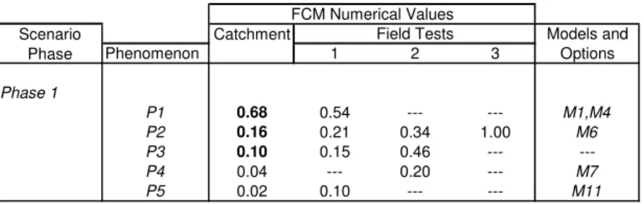
catchment for assessing the adequacy of the computer model for a specified application. The matrix in Table 2 is an extension of that shown in Table 1 with FCM values for a set of three field tests (1, 2, 3), with dashed lines indicating that the phenomenon for that row was not present in that test (or no related measurements were accurately taken).
From the previous example, it was determined that Phenomena P1, P2, and P3 are considered important for the application. A quick scan of these three rows indicates that only Field Test 1 has the presence of all these phenomena. For assessing a computer model, it is not only important to demonstrate the adequacy of simulating each significant phenomenon but also the
interactions among these phenomena as the catchment responds to the weather event. Field Test 1 is the only test that can provide the assessment of the computer model’s ability to simulate the phenomena interactions. For Field Test 2, Phenomenon P1 is absent (or not measured) and the ranking of P2 and P3 is reversed to that of the catchment. This indicates that it cannot be used to assess the interaction among the dominant phenomena but it could be used to assess P2 or P3 separately. Field Test 3 can only be used to assess the capabilities of the computer model to simulate Phenomenon P2.
The ranking of the dominant phenomena for the catchment provides the first cut for selecting appropriate field tests. The next step is to evaluate the scaling distortions in those field tests that made the cut. If a field test contains a significant scaling distortion in a dominant phenomenon then that test cannot adequately demonstrate the computer model’s ability to predict that
phenomenon. A phenomenon in a field test is well scaled if its representative FCM (the Π-value from Equation 10) has nearly the same numerical value as the FCM for the catchment. This is shown in Equation (12) where ΠC,P is the FCM of Phenomenon P for the catchment and ΠFT,P is its FRM for a field test:
1 , , ≅ Π Π P C P FT (12)
Exact similitude between a catchment and a field test for all dominant phenomena cannot be expected and it is not necessary for assessing the adequacy of a computer model. The challenge is to define an acceptable range of distortion, i.e., the a and b values that are shown in
Equation (13). b a P C P FT ≤ Π Π ≤ , , (13)
Determining an acceptable range of scaling distortion adds a degree of subjectivity to adequacy assessment for computer models. However, by quantifying and justifying this range along with the FCM values for the catchment and the field tests, one produces an assessment that is
traceable and auditable. By calculating the scaling distortions in the dominant phenomena for the field tests, one can select those tests that are best suited for assessing the adequacy of the
computer models.
It is important to note that the models and options that will be used in the simulation for the catchment must also be used for the simulations of the field tests. For example in Table 2, there are two model options - M1 or M4 - that can be used to simulate Phenomenon P1. Once M1 or M4 is selected it must be used for all field tests because the objective is to assess that model. The same rationale applies to the selection of model options.
As shown in this section, the ability to quantitatively rank phenomena provides a mechanism for efficiently selecting the appropriate stormwater models for a defined application. It also
and climate change applications where there are no direct measurements from the system, this capability means that existing data could be used to assess the adequacy of computer models if it can be demonstrated that there is minimal scaling distortions in the data.
6. CONCLUDING REMARKS AND FUTURE WORK
Some readers may question the need to go through the identification and ranking procedure that was presented in this report to arrive at conclusions that, for many situations, could be arrived at by expert judgment. As stated in the introduction to this report, the main anticipated use of this procedure is to qualify computer models for their capabilities to predict what would happen as a result of changes in land-use or climate. An important part of this qualification is to justify the assumptions that will be used. Often in modeling, many assumptions are made as input files are created and debugged but the rationales for them are not recorded. Also modelers sometimes make use of “hand-me-down” sections of input files, especially for large problems, and they do not always revisit the selected models and their options for the use on their particular problem. The identification and ranking procedure provides a framework for modelers to efficiently walk through a scenario and establish those phenomena that need to be accurately modeled before proceeding with the modeling analysis. The procedure also provides a traceable and auditable record of this process.
Another important step in the qualification of a computer model for an application is to compare its results to measured data. For predicting the effects of changes in land-use or climate, a priori measurements cannot be obtained from the changed system. However, the Fractional Scaling Analysis (FSA) method can be used to identify field tests that exhibit sufficient similarity in the important phenomena that are expected to occur in the changed system. The measured data from these field tests can then be used to assess the capabilities of the computer models to predict the effects of these changes.
This report provides an overview for a procedure to identify and rank rainfall and runoff
phenomena. There remain specific details to fill in and a proof of concept using actual scenarios and field data. The next step will be to derive the necessary balance equations for the overland flow on an urban drainage catchment using the integral form in Equation (1). The
Representative Elementary Watershed (REW) model (Reggiani et al., 1998, 1999; Reggiani and Rientjes, 2005; Zhang and Savenije, 2005) will be investigated for this purpose in future studies. In the REW model, a natural watershed is segmented into a set of interconnected sub-watersheds, called the REWs, using the stream channel network as the organizing structure. Each REW is represented as an open thermodynamic system with exchanges of mass, momentum, energy, and entropy with the atmosphere and surrounding regions (including other REWs). Atmospheric forcing processes (rainfall, solar radiation) and gravity (run-off, channel flow) drive these exchanges. Each REW is formulated to preserve an autonomous, functional watershed unit. Thus, the smallest permissible size of a REW is that which contains all the sub-regions. Each REW contains five major functional modules of a watershed: a saturated zone, an
unsaturated zone, a channel reach, and two overland flow zones – one over the unsaturated zone, the other over the saturated zone. Integral formulations of the balance equations, similar to the form in Equation (1), are derived for the five modules (Reggiani et al., 1998) with prescribed closure properties that are based on the second law of thermodynamics (Reggiani et al., 1999). Future work will look at extending the REW concept to urban drainage catchments, initially looking at overland flow. This will require re-defining the overland flow zones to accommodate urban settings, i.e., varying degrees of infiltration capacities (including impervious areas) and minor drainage structures. Once the appropriate balance equations are derived, they will be put
into non-dimensional form so that phenomena identification and ranking can be done for selected scenarios.
Work will also commence on selecting case studies from Canadian municipalities to evaluate the identification and ranking process. Along with the selection of evaluation cases, work will also be conducted to find suitable field data to evaluate selected stormwater models.
7. ACKNOWLEDGEMENTS
The National Research Council of Canada funded this work through the Institute for Research in Construction’s Urban Infrastructure (UI) Program, at the Centre for Sustainable Infrastructure Research (CSIR) in Regina, Saskatchewan. The author would like to thank Dr. Maruf Mortula (NRC-CSIR), Dr. David Hubble (NRC-CSIR) and Dr. Yehuda Kleiner (NRC-UI) for their insightful comments.
8. REFERENCES
Boyak B.E., Catton I., Duffey R.B., Griffith P., Katsma K.R., Lellouche G.S., Levy S., Rohatgi U.S., Wilson G.E., Wulff W., Zuber N., 1990. Qualifying reactor safety margins Part 1: an overview of the code scaling, applicability, and uncertainty evaluation methodology, Nuclear Engineering and Design, Vol. 119, pp 1-15
Ewen J. and Parkin G., 1996. Validation of catchment models for predicting land-use and climate change impacts. 1. Method, Journal of Hydrology, Vol. 175, pp 583-594
James W., 2005. Rules for Responsible Modeling, Fourth Edition, Computational Hydraulics International, ISBN 0-9683681-5-8
O’Connell P.E. and Todini E., 1996. Modeling of rainfall, flow, and mass transport in hydrological systems: an overview, Journal of Hydrology, Vol. 175, pp 3-16
Reggiani P., Sivapalan M., and Hassanizadeh S.M., 1998. A unifying framework for watershed thermodynamics: balance equations for mass, momentum, energy and entropy, and the second law of thermodynamics, Advances in Water Resources, Vol. 22(4), pp 367-398 Reggiani P., Hassanizadeh S.M., Sivapalan M., and Gray W.G., 1999. A unifying framework for
watershed thermodynamics: constitutive relationships, Advances in Water Resources, Vol. 23(1), pp 15-39
Reggiani P. and Rientjes, T.H.M., 2005. Flux parameterization in the representative elementary watershed approach: Application to a natural basin, Water Resources Research, Vol. 41, W04013
Weinberg G.M., 1975. An introduction to general systems thinking, John Wiley, New York, ISBN 0-471-92563-2
Wilson G.E. and Boyak B.E., 1998. The role of the PIRT process in experiments, code development and code applications associated with reactor safety analysis, Nuclear Engineering and Design, Vol. 186, pp 23-37
Wulff W., 1996. Scaling of thermalhydraulic systems, Nuclear Engineering and Design, Vol 163, pp 359-395
Wulff W., Zuber N., Rohatgi U.S., and Catton I., 2005. Application of Fractional Scaling
Analysis (FSA) to Loss of Coolant Accidents (LOCA) Part 2: System Level Scaling for System Depressurization, In: Proceedings of the 11th International Topical Meeting on Nuclear Reactor Thermal-Hydraulics (NURETH-11), Avignon, France, October 2-6 Zhang G.P. and Savenije H.H.G., 2005. Rainfall-runoff modeling in a catchment with a complex
groundwater flow system: application of the Representative Elementary Watershed (REW) approach, Hydrology and Earth Systems Science Discussions, Vol. 2, pp 639-690
Zuber N., Wilson G.E., Ishii M., Wulff W., Boyak B.E., Dukler A.E., Griffith P., Healzer J.M., Henry R.E., Lehner J.R., Levy S., Moody F.J., Pilch M., Sehgal B.R., Spencer B.W., Theofanous T.G., Valante J., 1998. An integrated structure and scaling methodology for severe accident resolution: Development of methodology, Nuclear Engineering and Design, Vol. 186(1-2), pp 1-21
Zuber N., 1999. A general method for scaling and analyzing transport processes, In: Applied Optical Measurements, Lehner M., Mewes D., Tauscher R., and Dinglreiter U. (Eds), Springer Verlag, Berlin
Zuber N. 2001. The effects of complexity, of simplicity, and of scaling in thermal-hydraulics, Nuclear Engineering and Design, Vol. 204(1), pp 1-27
Zuber N., Wulff, W., Rohatgi U.S., and Catton I., 2005. Application of Fractional Scaling Analysis (FSA) to Loss of Coolant Accidents (LOCA) Part 1: Methodology Development, In: Proceedings of the 11th International Topical Meeting on Nuclear Reactor Thermal-Hydraulics (NURETH-11), Avignon, France, October 2-6
Table 1: Matrix of phenomena rankings and models Phase 1 P1 0.68 M1,M4 P2 0.16 M6 P3 0.10 ---P4 0.04 M7 P5 0.02 M11 Models and Options Scenario Phase FCM Phenomenon
Table 2: Matrix of phenomena rankings for a catchment and three field tests
Phenomenon 1 2 3 Phase 1 P1 0.68 0.54 --- --- M1,M4 P2 0.16 0.21 0.34 1.00 M6 P3 0.10 0.15 0.46 --- ---P4 0.04 --- 0.20 --- M7 P5 0.02 0.10 --- --- M11 Scenario Phase Field Tests FCM Numerical Values Models and Options Catchment
Element 1 Establish Requirements
1. Specify urban drainage catchment 2. Specify primary evaluation criteria 3. Specify weather event(s)
4. Identify and rank dominant phenomena
Element 2
Develop Database of Applicable Field Experiments
5. Develop similarity criteria for the dominant phenomena identified in Element 1.
6. Identify candidate field data that will be compared against model predictions. Examine measurement uncertainties to determine if they are acceptable. 7. Perform scaling studies on the data and
determine if distortions are within acceptable limits.
8. Determine if there is sufficient qualified data to complete the adequacy assessment or if additional field data is required.
Element 3 Select Computer Model(s)
9. Evaluate the capability of each model and its numerical solution to simulate the phenomena that are identified in Element 1.
10. Assess the applicability of any closure relations to conditions defined in Element 1.
Element 4 Assess Adequacy of Model(s)
11. Prepare model input for the field experiments that were identified in Element 2. 12. Complete model calculations
of the experiments and compare to field measurements.
13. Determine the uncertainties in the model calculations for the primary evaluation criteria that were identified in Element 1.
Adequacy Decision
Have the capabilities of the model(s) been adequately
demonstrated?
YES NO
Proceed with analyses. Address deficiencies in the models (return
to Element 3) or in the field data (return to Element 2) and revise adequacy
assessment.
Rainfall Infiltration Evapotranspiration Mass Water Lawn Pervious Region Sub-catchment Urban Drainage Catchment
Phenomena Fields Constituents Components Modules Subsystems System
Rainfall Infiltration Evapotranspiration Mass
Water Lawn Pervious Region
Sub-catchment Urban Drainage Catchment
Phenomena Fields Constituents Components Modules Subsystems System