Phase lV experimental uncertainty analysis for ice tank ship resistance and manoeuvring experiments using PMM

Texte intégral

(1)NRC Publications Archive Archives des publications du CNRC. Phase lV experimental uncertainty analysis for ice tank ship resistance and manoeuvring experiments using PMM Lau, M.; Derradji-Aouat, A.. For the publisher’s version, please access the DOI link below./ Pour consulter la version de l’éditeur, utilisez le lien DOI ci-dessous.. Publisher’s version / Version de l'éditeur: https://doi.org/10.4224/8895111. Technical Report (National Research Council of Canada. Institute for Ocean Technology); no. TR-2006-03, 2006 NRC Publications Archive Record / Notice des Archives des publications du CNRC : https://nrc-publications.canada.ca/eng/view/object/?id=fcda9bae-e0bd-4266-9701-810c79152d60 https://publications-cnrc.canada.ca/fra/voir/objet/?id=fcda9bae-e0bd-4266-9701-810c79152d60 Access and use of this website and the material on it are subject to the Terms and Conditions set forth at https://nrc-publications.canada.ca/eng/copyright READ THESE TERMS AND CONDITIONS CAREFULLY BEFORE USING THIS WEBSITE. L’accès à ce site Web et l’utilisation de son contenu sont assujettis aux conditions présentées dans le site https://publications-cnrc.canada.ca/fra/droits LISEZ CES CONDITIONS ATTENTIVEMENT AVANT D’UTILISER CE SITE WEB. Questions? Contact the NRC Publications Archive team at PublicationsArchive-ArchivesPublications@nrc-cnrc.gc.ca. If you wish to email the authors directly, please see the first page of the publication for their contact information. Vous avez des questions? Nous pouvons vous aider. Pour communiquer directement avec un auteur, consultez la première page de la revue dans laquelle son article a été publié afin de trouver ses coordonnées. Si vous n’arrivez pas à les repérer, communiquez avec nous à PublicationsArchive-ArchivesPublications@nrc-cnrc.gc.ca..

(2) DOCUMENTATION PAGE REPORT NUMBER. NRC REPORT NUMBER. DATE. TR-2006-03. January, 2004. REPORT SECURITY CLASSIFICATION. Unlimited. Unclassified TITLE. Phase IV Experimental Uncertainty Analysis for Ice Tank Ship Resistance and Manoeuvring Experiments using PMM AUTHOR(S). Michael Lau and Ahmed Derradji-Aouat CORPORATE AUTHOR(S)/PERFORMING AGENCY(S). Institute for Ocean Technology PUBLICATION. SPONSORING AGENCY(S). Institute for Ocean Technology, Marine Institute IMD PROJECT NUMBER. NRC FILE NUMBER. 42_953_10 KEY WORDS. PAGES. FIGS.. TABLES. uncertainty analysis, PMM, manoeuvring, ice, Terry Fox. 72. 18. 14. SUMMARY. The Institute for Ocean Technology (IOT) of the National Research Council of Canada (http://www.iot-ito.nrc-cnrc.gc.ca/) has conducted physical, numerical and mathematical modeling of ship manoeuvring characteristics in ice, as part of a larger effort to develop reliable modeling techniques to assist in the design of new iceworthy vessels and in the simulation of their navigating characteristics. Preliminary tests were conducted for a range of model speeds and radii and an Experimental Uncertainty Analysis (EUA) was conducted on this test series as part of the data analysis. This report describes the model test program, and the results of the EUA. For consistency, this test series is referred to as Phase IV of the EUA.. ADDRESS. National Research Council Institute for Ocean Technology P. O. Box 12093, Station 'A' St. John's, Newfoundland, Canada A1B 3T5. Tel.: (709) 772-5185, Fax: (709) 772-2462.

(3) National Research Council Conseil national de recherches Canada Canada Institute for Ocean Technology. Institut des technologies océaniques. PHASE IV EXPERIMENTAL UNCERTAINTY ANALYSIS FOR ICE TANK SHIP RESISTANCE AND MANOEUVRING EXPERIMENTS USING PMM. Michael Lau and Ahmed Derradji-Aouat. January 2006.

(4) ABSTRACT The Institute for Ocean Technology (IOT) of the National Research Council of Canada (http://www.iot-ito.nrc-cnrc.gc.ca/) has conducted physical, numerical and mathematical modeling of ship manoeuvring characteristics in ice, as part of a larger effort to develop reliable modeling techniques to assist in the design of new iceworthy vessels and in the simulation of their navigating characteristics. Preliminary tests were conducted for a range of model speeds and radii and an Experimental Uncertainty Analysis (EUA) was conducted on this test series as part of the data analysis. This report describes the model test program, and the results of the EUA. For consistency, this test series is referred to as Phase IV of the EUA.. i.

(5) ACKNOWLEDGMENTS The investigations presented in this report were partially funded by the Atlantic Innovation Fund through the Marine Institute, Newfoundland. Work term student A. van Thiel provided assistance in performing the experimental uncertainty analysis. Their support is gratefully acknowledged.. ii.

(6) TABLE OF CONTENTS APPENDICES.............................................................................................................. iii LIST OF TABLES......................................................................................................... iv LIST OF FIGURES ...................................................................................................... iv 1.0 INTRODUCTION................................................................................................1 2.0 TESTS PROGRAMS..........................................................................................2 2.1 Test Set-up.........................................................................................................2 2.1.1 Ice tank....................................................................................................2 2.1.2 Terry Fox ship model...............................................................................2 2.1.3 Planar Motion Mechanism (PMM) ...........................................................3 2.1.4 Data Acquisition System (DAS) and video ..............................................3 2.2 Ice Conditions ....................................................................................................3 2.3 Test Matrix .........................................................................................................4 2.4 Description of the Experiments in Ice .................................................................4 2.5 Description of the Experiments in Open Water ..................................................5 3.0 TEST RESULTS ................................................................................................6 3.1 Resistance Tests................................................................................................6 3.2 Manoeuvring ......................................................................................................7 3.2.1 Tow forces...............................................................................................7 3.2.2 Yaw moments..........................................................................................8 4.0 EXPERIMENTAL UNCERTAINTY ANALYSIS (EUA) ......................................10 4.1 EUA for Ice Tank Testing – A Procedure Development ...................................10 4.2 EUA Procedure for Ice Tank Testing................................................................11 4.2.1 Segmentation hypothesis ......................................................................11 4.2.2 Steady state requirements.....................................................................13 4.3 Calculations for Random Uncertainties ............................................................17 4.3.1 Random uncertainties in resistance tests in ice.....................................18 4.3.2 Random uncertainties in manoeuvring tests in ice ................................18 4.3.3 Effect of correction for ice thickness on random uncertainties...............18 4.3.4 Effects of Data Reduction Equation (DRE)............................................19 4.4 Bias and Total Uncertainties ............................................................................19 4.5 Comparison with Previous Phases...................................................................19 5.0 CONCLUSIONS...............................................................................................21 REFERENCES ...........................................................................................................22. APPENDICES A. B. C. D. E. F.. Hydrostatics and particulars of the Terry Fox model Instrumentation and calibrations Ice sheet summaries Test matrix Channel width measurements in ice tests Typical test results. iii.

(7) LIST OF TABLES 1. PMM specifications 2. Change in tow force time history 3. Change in yaw moment time history 4. Change in model speed time history 5. Change in yaw rate time history 6. Change in drift angle time history 7. Mean thickness profiles 8. Mean flexural strength profile 9. Measured ice density values 10. Random Uncertainty in Phase IV resistance tests (tow force) 11. Random Uncertainty in Phase IV manoeuvring tests (tow force) 12. Chauvenet numbers 13. Random Uncertainty in Phase IV manoeuvring tests (yaw moment) 14. Effect of the DRE. LIST OF FIGURES 1. Terry Fox ship model 2. Planar Motion Mechanism 3. Typical test run in ice 4. Phase IV results from baseline open water tests 5. Phase IV results from ice resistance tests 6. Phase IV results from open water manoeuvring tests (tow force) 7. Phase IV results from ice manoeuvring tests (tow force) 8. Phase IV results from open water manoeuvring tests (yaw moment) 9. Phase IV results from ice manoeuvring tests (yaw moment) 10. Tow force and yaw moment -time history 11. Velocity-time history 12. Yaw rate-time history 13. Drift angle-time history 14. Ice thickness profiles 15. Corrected versus measured (uncorrected) mean tow force. 16. Flexural strength profiles 17. Measured density values 18. Comparison between corrected and uncorrected random uncertainties in mean tow force for resistance and manoeuvring tests. iv.

(8) PHASE IV EXPERIMENTAL UNCERTAINTY ANALYSIS FOR ICE TANK SHIP RESISTANCE AND MANOEUVRING EXPERIMENTS USING PMM 1.0 INTRODUCTION Recent development of offshore oil and gas reserves in several countries, together with economic studies to increase transportation through the Arctic, has led to a renewed interest in the manoeuvrability of vessels in ice. Despite a sizeable volume of work, there is not yet a universally accepted analytical method of predicting ship performance in ice. In 2003, the Institute for Ocean Technology (IOT) of the National Research Council of Canada (http://www.iot-ito.nrccnrc.gc.ca/) initiated a comprehensive physical, numerical and mathematical modeling of ship manoeuvring characteristics in ice, as part of a larger effort to develop reliable modeling techniques to assist in the design of new ice-worthy vessels and in the simulation of their navigating characteristics. Considering the complexity of the loads imposed by ice during ship manoeuvres, a preliminary series of ship manoeuvring experiments in ice were conducted for a range of model speeds and radii to provide insights to assist in the subsequent numerical and mathematical modeling. An Experimental Uncertainty Analysis (EUA) was conducted on the results of these tests as a step towards developing a procedure for EUA for ship manoeuvring in ice and to gain an acceptable level of confidence in the truthfulness of experimental results. As the objective of this series was primarily on the manoeuvring characteristics of vessels in ice, a full examination was not completed of the applicability of the EUA procedure as developed in Phases I to III of the EU project (Derradji-Aouat and van Thiel, 2004). However, EUA was performed to give a measure of the EU of the ice properties and the reported ice resistance and yaw moment data. This report accompanies IOT report TR-2006-02 (Lau and Derradji-Aouat, 2006), which documents the results of the manoeuvring tests, whereas this report documents the results of the EUA calculations. The description of the model test program is taken from TR-2006-02 for completion. Conclusions are made and recommendations for future works are provided. For consistency, this test series is referred to as Phase IV of the EUA.. 1.

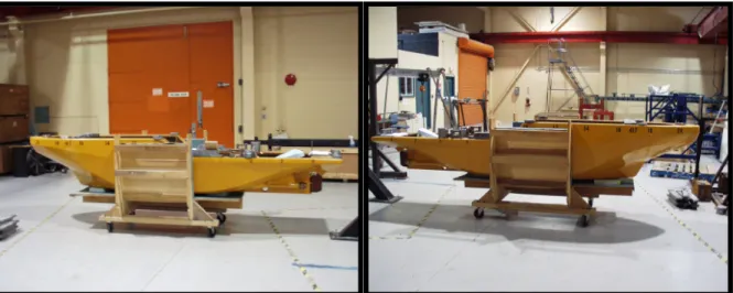
(9) 2.0 TESTS PROGRAMS In the ice tank, the Terry Fox model (scale = 1:21.8) was towed in five ice sheets using the PMM with the model restrained in roll. The model was outfitted with a rudder. Tests with different rudder angles were tested in open water only. Both moving straight and turning circle manoeuvres were tested. The target flexural strength and ice thickness of the ice sheets was the same for all experiments (35 kPa and 40 mm). During the turning circle manoeuvring tests, the drift angle β was set to zero degrees. Bubble ice was required for all ice sheets. Three different types of experiments were conducted. They were: 1) Experiments in Level Ice 2) Experiments in Pre-sawn Ice (Resistance runs only) 3) Experiments in Open Water 2.1. Test Set-up. In these tests, the main components of the test set up are the ice tank, the Terry Fox ship model, the Planar Motion Mechanism (PMM), the Data Acquisition System (DAS), and video cameras. 2.1.1 Ice tank The ice tank is 96 m long, 12 m wide and 3 m deep, with useable ice sheets of 76 m in length, making this tank the longest in the world. Thus, it allows for tests at higher speeds and longer test runs (more data is obtained per run). The 12 m width of the tank enables ship experiments in various manoeuvres, and for straight test runs in continuous ice, three tracks may be used (center channel, north quarter point and south quarter point) in each ice sheet. The ability to perform three continuous ice tests per sheet significantly improves the cost effectiveness. The effect of the tank walls on the center channel is also reduced because there is less confinement due to the tank walls with the wider ice tank. 2.1.2 Terry Fox ship model The experiments were carried out with a 1:21.8 scaled model of the Canadian Coast Guard’s icebreaker Terry Fox (IOT model # 417) (Figure 1). The model hydrostatics are provided in Appendix A. The model was mounted to the towing carriage through the PMM at the model’s center of gravity. The model was towed at a controlled planar motion through a level ice sheet. The model surface was finished to a friction coefficient of 0.01 with Dupont’s Imron paint.. 2.

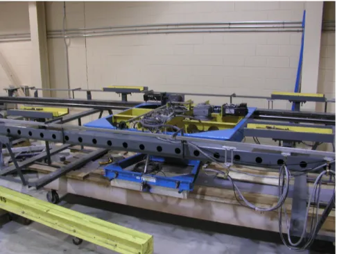
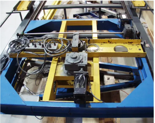
(10) 2.1.3 Planar Motion Mechanism (PMM) Marineering Limited (1997) provided details on the development and commissioning of the PMM. The PMM was designed to study the manoeuvring of ships in both ice and open water. The PMM apparatus (Figure 2) consists of two primary components: a sway subcarriage that is mounted beneath the main towing carriage, and a yaw assembly that is connected to the sway sub-carriage. The apparatus allows the model to yaw and sway in a controlled manner, while measuring the sway and surge forces as well as the yaw moment. The combination of sway and yaw allows a variety of manoeuvres to be performed. The PMM dynamometer has 3 cantilever-type load cells for measuring surge force, sway force, and yaw moment. A load cell aligned along the model’s surge axis measures surge force. The other two load cells aligned along the model’s sway axis measure sway force. Yaw moment is measured by resolving the outputs from the two sway load cells. The specifications for the PMM are given in Table 1. 2.1.4 Data Acquisition System (DAS) and video In each experiment, tow force, turning moment, and ship motions were measured. The transducer for outputs were sampled digitally at 50 Hz and filtered at 200 Hz. Two video recordings were made of each test, one on the starboard side that is manually controlled to follow the model’s manoeuvres, and the other looking down ahead of the model at the port side. All details regarding the instrumentation used in this test program and their calibration sheets are provided in Appendix B. 2.2. Ice Conditions. The experiments were carried out in CD-EG/AD/S ice (Spencer and Timco, 1990). With inclusions of air bubbles into the growing ice sheet, the model ice significantly improves the scaling of ice density, elastic, and fracture properties. For each ice sheet, flexural, compressive, and shear strengths were measured frequently throughout the test period. Strength versus time curves were created for each ice sheet and the strength values reported at each test time were interpolated from these curves. Flexural strength, σ f, was measured using in-situ cantilever beams. A number of shear strength measurements were performed immediately after the flexural strength test to provided index values for. 3.

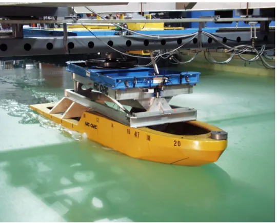
(11) comparison with the measured flexural strengths. The ratio of shear strength to downward breaking flexural strength varied from 1.03 to 3.16. The reported ice thickness, h, is the average thickness of approximately 65 measurements of the ice sheet thickness along the test path. The IOT standards and work procedures were followed for producing and characterizing level ice sheets. All work procedures are given in the IOT documentations for system quality. The procedures followed to prepare the ice tank, seed and grow the ice sheet are given in the IOT work procedures TNK 22, TNK 23, and TNK 37, respectively. The mechanical properties of the ice are determined according to the following work procedures: TNK 26 (for measuring the flexural strength), TNK 27 (for measuring the elastic modulus), TNK 28 (for measuring compressive strength), and TNK 30 (for measuring ice density). Ice thickness measurements were performed as per the work procedure TNK 25. It should be noted that all of the above work procedures are valid for both bubbly ice and non-bubbly ice. Simply, in the case of non-bubbly ice, the bubbler system is turned off. The test program required five (5) different ice sheets with a nominal thickness of 40 mm and a nominal flexural strength of 35 kPa at beginning of test day. The flexural strengths were tempered throughout the test day. A summary of the five ice sheets and their properties are presented in Appendix C. 2.3. Test Matrix. The overall test matrix is summarized in Appendix D. For the tests described in this program, the ice sheets had a target ice thickness of 40 mm and a target flexural strength of 35 kPa. The following manoeuvres were utilized: (1) resistance runs in which the model was towed along a straight line at a zero drift angle, and (2) pure yaw through a constant radius manoeuvre so that the heading of the model was always tangential to the path of its center of gravity resulting in zero sway force and a yaw moment. All tests in ice were performed with a zero degree rudder angle and a model velocity ranging from 0.02 m/s to 0.6 m/s. The constant radius manoeuvre was conducted with two turning radii (50 m and 10 m). Additional resistance tests were also conducted at a model velocity of 0.9 m/s. Concurrent to the testing in ice, manoeuvres in open water were also conducted. The open water runs were performed with a rudder angle of 0, 20, and 30 degrees. 2.4. Description of the Experiments in Ice. The experiments conducted in ice included level ice resistance runs, pre-sawn ice resistance runs, and arc manoeuvring runs in level ice. Figure 3 shows a. 4.

(12) picture of a typical test run in ice. Ship model speeds of 0.02 m/s, 0.05 m/s, 0.1 m/s, 0.2 m/s, 0.3 m/s, 0.4 m/s, 0.5 m/s, 0.6 m/s, and 0.9 m/s were tested in ice (see Appendix D). Appendix E summarizes the channel width measurements obtained in ice tests and shows the run schematics for manoeuvring tests in ice. Figures E.1 to E.5 show schematics for the ice test runs in each sheet. For the first ice sheet, NMS1, the runs conducted are shown in Figure E.1. The second ice sheet, NMS2, used the same test matrix as Runs 1- 3 for Phase III (Figure E.2). The schematics for the ice sheets NMS3, NMS4 and NMS5 are shown in Figures E.3, E.4, and E.5, respectively. For the straight runs, the following test run scenario was performed in the first two ice sheets (NMS1 and NMS2). Initially, a level ice test run was conducted along the centerline of the tank. In NMS1, the model was towed at a constant speed of 0.1, 0.6 and 0.9 m/s with an approximately 20 m run distance each, and a creep test performed at the end (0.02 m/s). Afterwards, the model was tested at the quarter-point (on either side of the center-line). Again, the model was towed at the set constant speeds of 0.1, 0.6, 0.9, and 0.02 m/s (creep speed). For the south quarter point test, a pre-sawn ice test run was performed (same procedure as per the standard resistance test). In NMS2, the same schematic was used and speeds tested were 0.1, 0.3, and 0.6 m/s, followed by a creep test. For turning circle tests, the model was towed at a constant yaw rate with the prescribed arc radius (10 m and 50 m) and run length. The runs were conducted in the last three ice sheets (NMS3, NMS4 and NMS5). 2.5. Description of the Experiments in Open Water. The open water tests for the corresponding ice test runs were baseline open water tests. The experiments conducted in open water included resistance runs and arc manoeuvring. Ship model speeds of 0.02 m/s, 0.05 m/s, 0.1 m/s, 0.2 m/s, 0.3 m/s, 0.4 m/s, 0.5 m/s, 0.6 m/s and 0.9 m/s were tested with three rudder angles (0, 20, and 30 degrees) (See Appendix D). Note that all open water tests were conducted in the ice tank, for calm water conditions (no waves).. 5.

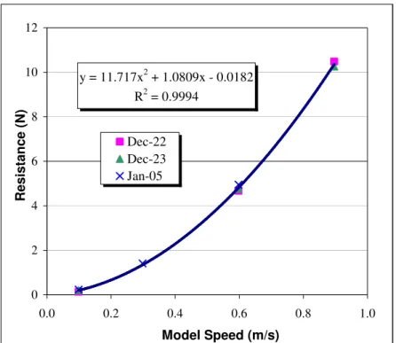
(13) 3.0 TEST RESULTS Plots for typical test results are given in Appendix F. 3.1. Resistance Tests. Open water Baseline open water resistance tests were completed in the ice tank for test speeds corresponding to the ice tests conducted. Figure 4 shows the measured tow force versus model velocity for the open water resistance runs. The numerical values for the mean tow force at each speed are: Model Velocity Mean Tow Force (m/s) (N) 0.1 0.18 0.3 1.41 0.6 4.81 0.9 10.48 The resistance (given in N) in baseline open water, Row, can be obtained from the regression line in Figure 4: Row = 11.717·V2 + 1.0809·V - 0.0182. (1). where V is the tow velocity (in m/s). Ice Tests Figure 5 shows the measured tow force versus model velocity for the resistance tests in both pre-sawn and continuous ice. The numerical values for the mean tow force at each speed are: Presawn Ice Level Ice Model Velocity Mean Tow Force Mean Tow Force (m/s) (N) (N) 0.02 4.50 9.02 0.1 5.95 10.38 0.3 9.01 15.74 0.6 16.36 23.85. 6.

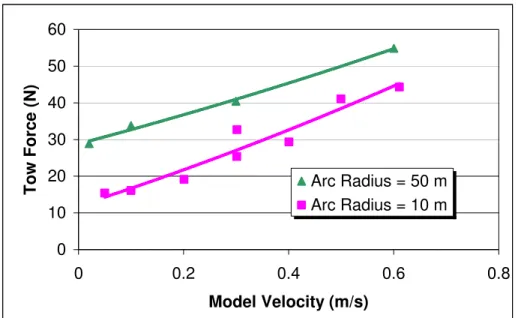
(14) 3.2. Manoeuvring. 3.2.1 Tow forces Open water Baseline open water manoeuvring tests were completed in the ice tank for test speeds corresponding to the ice tests conducted. Figure 6 shows the measured tow (surge) force versus model velocity curves for the open water manoeuvring runs grouped according to rudder angle. The numerical values for the mean tow (surge) force at each speed are: Rudder Angle Rudder Angle Rudder Angle 0 degrees 20 degrees 30 degrees Model Velocity Mean Surge Force Mean Surge Force Mean Surge Force (m/s) (N) (N) (N) R = 10 m R = 50 m R = 10 m R = 50 m R = 10 m R = 50 m 0.1 1.09 0.88 3.73 0.49 4.23 0.40 0.3 2.57 1.18 n/a n/a n/a n/a 0.6 8.43 4.54 12.11 7.51 14.65 8.92 0.9 42.79 10.50 27.36 14.52 25.53 19.41 The resistances in baseline open water manoeuvring, Row, for the two turning radii with zero rudder angle can be obtained from the regression lines in Figure 6: Arc radius = 10m Row = - 33.135·V2 + 5.4·V + 0.6609. (2a). Arc radius = 50m Row = -13.653·V2 + 0.4821·V+ 0.1673. (2b). Ice tests Figure 7 shows the measured tow force versus model velocity curves for the ice manoeuvring runs. The results for Runs 132, 133, 148, and 153 are not shown, as those measurements were suspicious due to problem with the model’s initial alignment. These results were not corrected for ice strength, which may contribute to the scattering of data. The numerical values for the mean tow (surge) force at each speed are:. 7.

(15) Level Ice Mean Surge Force (N) R = 10 R = 50 m m n/a 28.91 15.43 n/a 16.11 33.82 19.12 n/a 29.01 40.42 29.33 n/a 41.08 n/a. Model Velocity (m/s) 0.05 0.1 0.2 0.3 0.4 0.5 0.6 3.2.2 Yaw moments. Open water Figure 8 shows the measured yaw moment versus model yaw rate curves for the open water manoeuvring runs grouped according to rudder angle. The numerical values for the mean yaw moment at each model speed1 are: Rudder Angle Rudder Angle Rudder Angle 0 degrees 20 degrees 30 degrees Model Velocity Mean Yaw Mean Yaw Mean Yaw (m/s) Moment (Nm) Moment (Nm) Moment (Nm) R = 10 m R = 50 m R = 10 m R = 50 m R = 10 m R = 50 m 0.1 0.93 0.07 3.04 -0.04 3.39 0.09 0.3 -0.63 -0.90 n/a n/a n/a n/a 0.6 -7.96 -4.47 -5.06 -4.96 -5.99 -5.27 0.9 -21.02 -10.41 -23.30 -10.54 -24.45 -11.78 The yaw moment (given in N·m) in baseline open water manoeuvring, Now, for the 2 turning radii with zero rudder angle can be obtained from the regression lines in Figure 8: Now = 0.4516·r2 – 0.7781·r. (2c). where r is the yaw rate (in deg/s). Ice Tests Figure 9 shows the measured yaw moment versus model yaw rate curves for the ice manoeuvring runs. The results for Runs 132, 133, 148, and 153 are not shown, as those measurements were suspicious due to problems with the 1. Yaw Rate = Model Speed / Turning Radius. 8.

(16) model’s initial alignment. These results were not corrected for ice strength, which may contribute to the scattering of data. The numerical values for the mean yaw moment at each speed are:. Level Ice Mean Yaw Model Velocity Moment (Nm) (m/s) R = 10 R = 50 m m 0.02 n/a 15.86 0.05 67.91 n/a 0.1 77.58 38.24 0.2 84.26 n/a 0.3 113.52 25.96 0.4 93.42 n/a 0.5 114.19 n/a 0.6 123.00 84.81. 9.

(17) 4.0 EXPERIMENTAL UNCERTAINTY ANALYSIS (EUA) Experimental Uncertainty Analysis is used to gain an acceptable level of confidence in the truthfulness of experimental results. As the objective of this series was primarily on the manoeuvring characteristics of vessels in ice, a full examination was not completed of the applicability of the EUA procedure as developed in Phases I to III of the EU project (Derradji-Aouat and van Thiel, 2004). However, EUA was performed to give a measure of the EU of the ice properties and the reported ice resistance data. For consistency, this test series is referred to as Phase IV of the EUA. 4.1. EUA for Ice Tank Testing – A Procedure Development. A literature review of the history and development of EUA in marine/ocean testing facilities was given by Derradji-Aouat (2002) and the mathematical basis of the EUA procedure was adopted from Coleman and Steele (1998). In a typical experiment, the total uncertainty, U, is the geometric sum of a bias uncertainty component, B, and a random uncertainty component, P: U =±. (B. 2. + P2. ). (3). The bias component, B, consists of uncertainties in instrumentation and equipment calibrations. Examples of bias uncertainty sources are the load cells, RVDT’s (Rotary Variable Differential Transformers), yoyo potentiometers, and the Data Acquisition System (DAS). On the other hand, the precision component, P, deals with environmental and human factors that may affect the repeatability of the test results (i.e. if a test was to be repeated several times, would the same results be obtained each time?). Examples of random uncertainty sources are the changing test environment (such as fluctuations in room temperature during testing), small misalignments in the initial test setup, human factors, etc. Derradji-Aouat (2002) showed that in a typical ice tank ship resistance test, the bias uncertainty component B is much smaller than the random uncertainty component P. He reported that, in Phase I ship model tests in ice, the value of B is at least one order of magnitude smaller than the value of P. He concluded, therefore, that in routine ship resistance ice tank testing, the total uncertainty U can be taken as equal to the random uncertainty component. Simply, without a loss of accuracy, the bias uncertainty component can be neglected. It follows that: U = ±P. 10. (4).

(18) 4.2. EUA Procedure for Ice Tank Testing. There are two major considerations when applying the EUA procedure to ice tank testing: the segmentation hypothesis and the steady state requirement. 4.2.1 Segmentation hypothesis For the ice test runs, several factors have contributed to the decision for keeping the speed of the ship model constant for a longer length than required for a test run, i.e., > 1.5 times the length of the model as required by the ITTC (ITTC, 2002). The main hypothesis is that the time history from one long test run can be divided into segments, and each segment can be analyzed as a statistically independent test. The hypothesis states that (Derradji-Aouat, 2002 and 2003, and Derradji-Aouat and van Thiel, 2004): “The history for a measured parameter (such as tow force versus time) can be divided into 10 (or more) segments, and each segment is analyzed as a statistically independent test. Therefore, the 10 segments in one long test run in ice are regarded as 10 individual (independent but identical) tests.” Coleman and Steel (1998) reported that, in statistical uncertainty analysis, a population of at least 10 measurements (10 data points) is needed. Precision uncertainty is calculated using the mean and the standard deviation of that population. However, in ice tank testing, it is recognized that conducting the same test 10 times is very costly and very time consuming. Therefore, the principle of segmenting the time history of a measured parameter over a long test run into multiple segments results in significant savings in project costs and efforts. By demonstrating that each segment can be analyzed as a statistically independent test, uncertainties are calculated from the means and standard deviations of the individual segments. The segmentation hypothesis is further illustrated in the Phase II report (Derradji-Aouat, 2003). Using the segments, the first calculation step is to obtain mean and standard deviation for each segment. The second step is to calculate the mean of the means and the standard deviation of the means. The mean of the means and standard deviation of the means are needed to compute random uncertainties in the results of the test run (as it will be shown in the subsequent sections). These two basic calculations steps are repeated for all test runs in all five (5) ice sheets. It should be cautioned that the segmentation hypothesis is valid only if the following three conditions are satisfied (Derradji-Aouat, 2004): 1) Each segment should span over 1.5 to 2.5 times the length of the ship model,. 11.

(19) 2) Each segment should include at least 10 events for ice breaking (10 load peaks) or at least 10 collision events (in the case of pack ice test runs), and 3) General trends (of a measured parameter such as tow force versus time) are repeated in each segment. Condition # 1 is based on the fact that the ITTC procedure for resistance tests in level ice (ITTC-4.9-03-03-04.2.1) requires that a test run should span over at least 1.5 times the model length. For high model speeds (> 1 m/s), however, the ITTC procedure requires test spans of 2.5 times the model length. Condition # 2 is based on the fact that in EUA, for an independent test, a population of at least 10 data points is needed to achieve the optimal value of 2 for the factor t (Coleman and Steele, 1998). For tests in ice tanks, 10 to 15 segments are recommended. The gain in any further reduction in the value of t (by having more than 10 to 15 segments) is minimal. Condition # 3 is introduced to ensure that the overall trends in a measurement (such as tow force versus time) are repeated in each segment. This condition serves to provide further assurance into the main hypothesis (“…Therefore, the 10 segments in one long test run are regarded as 10 individual, independent but identical, tests”). Fundamentally, if the trends are not repeated, reasonably, then the segments could not be analyzed as “independent but identical” tests. For these tests, Condition #1 was relaxed, as the shorter runs only allow for the extractions of a smaller numbers (up to 5) of repeating segments for each run. This will affect the calculations of the random uncertainties as explained in Section 4.3. It is important to emphasize the fact that the division of the time history of a measured parameter into consecutive segments is valid only for long test runs at constant speed and heading. If the model speed or heading is changed during the test run, then the segments cannot be analyzed as “identical”. Note that the time histories measured in creeping speed test are not subjected to the segmentation hypothesis. Furthermore, it is recognized that the division of the results of a test run into segments is valid only for the steady state portion of the measured data, and only the steady state portion of the measured time history is to be used. This is required to eliminate the effects of the initial ship penetration into the ice (transient stage), and the effects of the slowdown and full stop of the carriage during the final stages of the test run.. 12.

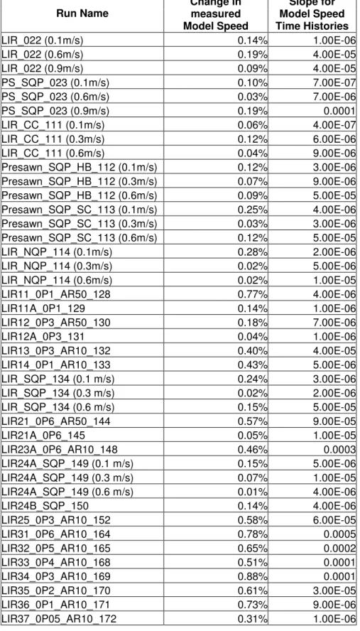
(20) 4.2.2 Steady state requirements In ice tank testing, for any given ice sheet, the ice properties are not completely uniform (same thickness) and homogeneous (same mechanical properties) throughout the ice sheet. This is attributed, mainly, to the ice growing processes and the refrigeration system in the ice tank. An example to illustrate the spatial variability of the material properties is provided by Derradji-Aouat and van Thiel (2004). In addition to the spatial variability of the material properties of ice during an ice test run, the carriage speed may or may not be maintained at exactly the required nominal constant speed2. Due to this inherent non-uniformity of ice sheets, the non-homogeneity of ice properties, and the small fluctuations in the carriage speed, a steady state condition in the time history of a measurement may not be achieved. Theoretically, if the time history of a measured parameter is changing drastically, then the segments could not be analyzed as “identical” tests (condition # 3). The steady state requirement, therefore, calls for a corrective action to account for the effects of non-uniform ice thickness, non-homogenous ice mechanical properties, and small fluctuations in carriage speed on the test measurements. To identify whether or not the time history for a measured parameter has reached its steady state, the following procedure was recommended (Derradji-Aouat, 2002). The measured time histories for all parameters were plotted along with their linear trend lines. A linear trend line with a zero slope (or a slope very close to zero) indicates that a steady state in a measured parameter is achieved. Figures 10a to 10f shows the time histories for the measured tow forces in Phase IV testing. Time histories for Phases I to III testing were provided in the previous reports by Derradji-Aouat (2002), Derradji-Aouat (2003) and Derradji-Aouat and van Thiel (2004), respectively. Figures 10g to 10h show the time histories for the measured yaw moments in Phase IV testing for the manoeuvring runs. After drawing the linear trend lines through all measured tow forces and yaw moments, it was observed that, in a majority of cases, a true steady state was never achieved (Tables 2 and 3). For example, the linear trend lines for representative tow force time histories are shown in Fig. 10. A steep sloping trend line reflects the fact that the tow force or yaw moment did not reach their steady state.. 2. The control system maintains the carriage speed; however, when ice breaks, small fluctuations in carriage speed may take place. 13.

(21) As shown in Tables 2 and 3, the non-steady state led to some significant changes in the tow forces and yaw moments over the towing distance (up to 284.83% and 49.38%, respectively). This non-steady state condition may be attributed to one (or all) of the following three factors: 1) A changing carriage speed (or small fluctuations in carriage speed) during testing, 2) Non-uniform ice thickness, and 3) Non-uniform mechanical properties of the ice (flexural/compressive strengths, elastic modulus, and density of ice). The contribution of each factor is further investigated as follows: Effects of changing model speed Figure 11 shows the time histories of the measured model speed in Phase IV testing. The linear trend lines point to the fact that, during testing, the actual changes in the model speed were very small and so, consequently, they can be neglected. Trend lines through the model velocity histories had slopes between 4 X 10-7 and 5 X 10-4. Table 4 shows that, over the towing distance for run with a particular velocity, the changes in the model velocity ranged between 0.01% and 0.88%. By and large, the model speed is very much steady, therefore, it was assumed that the contribution of the changing model speed into the development of nonsteady state time history of the measured parameters could be ignored. Consequently, no corrections for model speed fluctuations are needed. The same conclusions were reached in previous phases of testing (Derradji-Aouat, 2002 and 2003, and Derradji-Aouat and van Thiel, 2004). Effect of changing model yaw rate and drift angle in the manoeuvring runs The manoeuvring runs in this test series require the PMM to maintain a constant yaw rate and drift angle, in addition to a constant model (tangential) speed. Therefore, the controllability of the carriage on these two variables was assessed. Figure 12 shows the time histories of the measured yaw rate in Phase IV testing. The linear trend lines point to the fact that, during testing, the actual changes in the yaw rate were small and so, consequently, they can be neglected. Trend lines through the yaw rate histories had slopes between 2 X 10-6 and 0.0062, and the changes were larger with larger yaw rate as shown in Figure 12. Table 5 shows that, over the towing distance for run with a particular yaw rate, the changes in the yaw rate ranged between 0.27% and 2.66%. Figure 13 shows the time histories of the drift angle in Phase IV testing. The drift angle was computed as the difference between the targeted yaw angle. 14.

(22) (corresponding to zero drift angle)3 and the measured model yaw angle. The linear trend lines point to the fact that, during testing, the actual changes in the drift angle were not small and so, consequently, they cannot be neglected. Trend lines through the drift angle histories had slopes between 8 X 10-5 and 0.1862, and the changes were larger with larger yaw rate, as shown in Figure 13. Table 6 shows that, over the towing distance for run with a particular yaw rate, the changes in the drift angle ranged between 1.49% and 79.33%. It should be noticed that the derivation from the target drift angle (zero degree) increased with yaw rate (Lau and Derradji, 2004). Effects of non-uniform ice thickness Measured ice thickness profiles along the channels created by test runs in the ice tank are given in Figure 14a. Each profile consisted of a series of ice thickness measurements (every 2 m) along the length of the ice tank. Mean thickness profiles are given in Figure 14b, whereby each mean profile is the average of all measurements at the same tank length location. The linear trends, through the mean profiles, indicate that the ice thickness varied within the range of 4.36% (NMS3) to 8.02% (NMS2), as can be shown in Table 7. To correct for the effects of non-uniform ice thickness on the test measurements, the following correction methodology and rational are used (Derradji-Aouat, 2002): a. Uncertainty analyses for both mean and maximum tow forces may be calculated. In ice engineering, maximum tow forces are indicators for maximum ice loads on the ship structure, while mean tow forces are used in the standard ship resistance calculations. For this phase, only the mean tow force is examined. b. In the following discussion, mean ice resistance values are used to show how the EUA method is conceptualized and developed. The same procedure and equations are used for maximum ice resistance values (Derradji-Aouat, 2002). c. Ice thickness corrections are applied only to the resistance of ice. In ice resistance analysis, the total ice resistance, RIce, is equal to the measured resistance in ice tests, Rt, minus the resistance measured in the baseline open water tests, Row (Derradji-Aouat and van Thiel, 2004).. ( RIce ) Mean 3. =. ( Rt )Mean - ( Row ). The targeted yaw angle was computed from the PMM controlled model motion as follows:  Vy  Vx. β = tan −1 .   − rmeas . 15. (5).

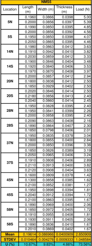
(23) where Row is obtained from the correlation obtained from the baseline open water test results. For resistance tests Equation 1 is used, and for manoeuvring tests with arc radii of 10m and 50 m, Equations 2a and 2b are used, respectively. d. For a given ice sheet, with nominal thickness ho, the following equation is used to calculate mean total ice resistance (Derradji-Aouat, 2003):. ( R Ice )Correct M ean = ( R Ice )M easured M ean ⋅ . ho    hm . (6). where (RIce) Correct Mean is the corrected total ice resistance for the nominal ice thickness ho (ho = 40 mm), (RIce) Measured Mean is the measured total ice resistance for the nominal ice thickness ho. The parameter hm is the ice thickness averaged over the measurements taken at an area within which the corresponding resistance time history segment is corrected. Note that Equations 5 and 6 are also valid when using maximum ice resistance values. This is achieved by substituting the subscript “mean” in Equations 5 and 6 by the subscript “max”. Figures 15a and 15b show the plots for corrected versus measured (uncorrected) mean tow force for the resistance and manoeuvring tests, respectively. Note that only the results of tests in continuous ice were subjected to ice thickness corrections. Note, also, that the time histories measured in the creeping speed test runs were not subjected to corrections for ice thickness variation. The length of each creeping speed test run was small (only one ship length ≈ 3.8 m), and the variation of ice thickness over this small length can be ignored. Effects of non-homogeneous ice properties Measured flexural strength profiles along the length of the ice tank are given in Figure 16a. Mean flexural strength profiles are given in Figure 16b. In-situ cantilever beam flexural strength measurements were conducted along the ice tank. The beam dimensions have the proportions of 1:2:5 (thickness: width: length). The flexural strength, σf, is calculated as:. σf =. 6PL whf 2. (7). where L is the length, w is the width, hf is the thickness, and P is the point load. The uncertainty in the measured flexural strength is Uσf:. 16.

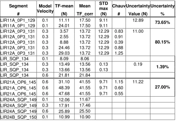
(24) Uσ f = UP2 + UL2 + UW2 + 2Uh2f. (8). where UL, UW, and Uhf are the uncertainties in the measured dimensions L, w and hf, respectively, and Up is the uncertainty in the measured point load. The uncertainties in the flexural strength profiles were calculated using Equation 14, and they are given in Table 8. Uncertainties varied between 33.03% and 88.44%. Measured ice density values in the ice tank are given in Table 9 and shown in Figure 17. The density of ice, ρi, is:. ρi = ρ w −. M V. (9). where ρw is the density of water. M and V are the mass and volume of the ice. The uncertainty involved in the ice density is: U ρ = UH2 + UL2 + UW2 + UM2 i. (10). The value of UM is neglected because it is considered a bias uncertainty (Derradji-Aouat, 2002). The variation of density in the ice tank ranged between 5.60% and 11.59%. From the ice tank operational point of view, in non-bubby ice sheets, density values could not be controlled but uniformity is reasonably assured. In bubbly-ice, however, the opposite is true, the target density values can be achieved but the spatial uniformity of the ice density is compromised. 4.3. Calculations for Random Uncertainties. Step # 1:. In Tables 10 and 11, after the calculations of the mean of means, Mean_TFMean, and standard deviation of means, STD_TFMean, the Chauvenet’s criterion was applied to identify the outliers (outliers are discarded data points). The Chauvenet number for mean tow forces is:. (Chauv # )Mean. =. TFMean -. ( Mean _TFMean ). (11). ( STD _TFMean ). The Chauvenet’s criterion dictates that the Chauv # for each data point should not exceed a certain prescribed value (Coleman and Steele, 1998). For 10 to 15 17.

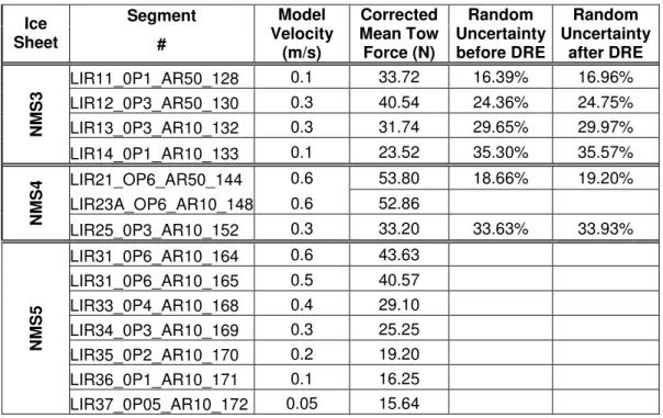
(25) segments, the Chauv # should not exceed 1.96 to 2.13. The Chauvenet numbers for other sample sizes are given in Table 12. A new mean of means and a new standard deviation of means were then calculated from the remaining data points (remaining segments). Step # 2:. After calculating the new mean of the means and the new standard deviation of the means (from the remaining segments - data points), random uncertainties in the mean tow force are:   t ⋅ ( STD_TFMean )  U(TFMean )  =   N  . (12). where the variable t is a function of the degrees of freedom and the confidence limit, and N is the number of the remaining data points (segments). For example, for a sample size N larger than 10 and a confidence limit of 95%, t is approximately equal to 2. Step # 3:. Random uncertainties, calculated using Equation 18, are expressed in terms of uncertainty percentage, UP:   UP(TFMean  .  U(TFMean ) ) = ⋅ 100  Mean_TFMean . (13). 4.3.1 Random uncertainties in resistance tests in ice The calculated uncertainties in mean resistance are summarized in Table 10. The uncertainties range from 0.53% to 80.15%. 4.3.2 Random uncertainties in manoeuvring tests in ice The calculated uncertainties in mean surge force are summarized in Table 11. The uncertainties range from 16.39% to 35.3%. The calculated uncertainties in mean yaw moment are summarized in Table 13. The uncertainties range from 10.01% to 62.96%. 4.3.3 Effect of correction for ice thickness on random uncertainties Corrections for variations in ice thickness profiles (using Equation 6) are made only for tests in continuous ice. Figures 18a and 18b show the comparison between corrected and uncorrected random uncertainties in mean tow force for. 18.

(26) resistance and manoeuvring tests, respectively. The correction for variation in ice thickness did not have much effect of the random uncertainty in both the resistance and manoeuvring tests. 4.3.4 Effects of Data Reduction Equation (DRE) Equation 6 was proposed to correct effects of ice thickness variations on the values of random uncertainties. It should be recognized that the corrected resistance curves are not direct laboratory measurements, but they are calculated from the analytical equation (Equation 6). The process of using analytical equations to correct measured parameters is called “Application of Data Reduction Equations (DRE)”. In EUA, there are additional random uncertainties involved in the application of the DRE. The uncertainty involved in using Equation 6 is: U R U R  0   =    R R    0. 1.   . 2. U +  h  h0.   . 2. 2   . (14). In the above equation, (UR/R) is the total uncertainty in resistance, R. Both (UR0/R0) and (Uh/h0) are the relative uncertainty in the measured ice resistance (as calculated in Tables 10 and 11), and the relative uncertainty in the measured ice thickness, respectively (the uncertainties in ice thickness are shown in Table 4). Note that, in Equation 14, the value of (Uh/h0) is an additional relative uncertainty, which is induced by the application of the DRE. The total relative uncertainty is the geometric sum of both relative uncertainties (UR0/R0) and (Uh/h0). Tables 14a and 14b summarize the mean tow forces, random uncertainties before and after the use of the DRE for the resistance and manoeuvring tests, respectively. After adding the effect of the DRE, in mean tow force, final uncertainties ranged between 4.58% and 80.27% for resistance tests and ranged between 16.96% and 35.57% for manoeuvring tests. 4.4. Bias and Total Uncertainties. In ice tank testing bias uncertainties are neglected (Derradji-Aouat, 2002), and therefore, the total uncertainties are taken as equal to the random ones. 4.5. Comparison with Previous Phases. Total uncertainties obtained in previous phases of testing were generally between 3% and 10% for continuous ice resistance tests. For Phase IV tests, the. 19.

(27) total uncertainties were mainly under 20% for resistance tests and mainly under 35% for manoeuvring tests. The uncertainties obtained in this phase of testing are generally larger than uncertainties calculated in previous phases; this is partially due to the fact than a smaller sample size was used (smaller number of segments) in Phase IV analysis. Another possible explanation may be the effect of the changing boundary conditions when performing arc tests. The model position relative to the tank wall changes during manoeuvring tests, therefore varying the ice boundary conditions. Boundary conditions may also be affected by the testing of several arcs in close proximity within an ice sheet.. 20.

(28) 5.0. CONCLUSIONS. A total of 42 ice test runs (using five different ice sheets) were used to generate data to analysis the manoeuvring characteristics (28 resistance test and 14 manoeuvring tests). The uncertainties obtained in this phase of testing are generally larger than uncertainties calculated in previous phases; this is partially due to the fact than a smaller sample size was used (smaller number of segments) in Phase IV analysis. The development of a EUA procedure for manoeuvring in ice is not possible due to the limited usable data currently available. The work completed for this test series is a preliminary analysis, as a step towards developing a EUA procedure for ice manoeuvring tests. Further manoeuvring tests are required to provide more data for EUA.. 21.

(29) REFERENCES Coleman, H. W. and Steele, W. G. (1998), “Experimentation and Uncertainty Analysis for Engineers.” 2nd edition, John Wiley & Sons publications, New York. Derradji-Aouat, A. (2002). “Experimental Uncertainty Analysis for Ice Tank Ship Resistance Experiments.” IMD/NRC report # TR-2002-04, Institute for Ocean Technology, St. John’s, Newfoundland. Derradji-Aouat, A. (2003). “Phase II Experimental Uncertainty Analysis for Ice Tank Ship Resistance Experiments.” IMD/NRC report # TR-2003-09, Institute for Ocean Technology, St. John’s, Newfoundland. Derradji-Aouat, A. (2004). “A Method for Calculations of Uncertainty in Ice Tank Ship Resistance Testing.” Proceedings of the 19th International Symposium on Sea Ice, Mombetsu, Japan. Derradji-Aouat, A. and van Thiel, A. (2004). “Terry Fox Resistance Tests – Phase III (PMM Testing). The ITTC Experimental Uncertainty Analysis Initiative.” IOT/NRC report # TR-2004-05, Institute for Ocean Technology, St. John’s, Newfoundland. ITTC (2002). “Testing and Extrapolation Methods, Ice Testing, Resistance Test in Level Ice.” ITTC Recommended Procedures, Section ITTC-4.9-03-03-04.2.1, ITTC. Lau, M. and Derradji-Aouat, A. (2004) “Preliminary Modelling of Ship Manoeuvring in Ice Using a PMM”, IOT/NRC report # TR-2006-02, Institute for Ocean Technology, St. John’s, Newfoundland. Marineering Limited (1997). “The Development and Commissioning of a Large Amplitude Planar Motion Mechanism. Volume 1: Main Report.” IMD/NRC report # CR-1997-05, Institute for Ocean Technology, St. John’s, Newfoundland. Spencer, D.S. and Timco, G.W. (1993) “CD Model Ice – A Process to Produce Correct Density (CD) Model Ice.” Proceedings of the 10th International IAHR Symposium on Ice, Vol. 2, Espoo, Finland, pp. 745-755.. 22.

(30) Table 1: Specifications of the PMM Max Sway Amplitude (m) Max Yaw Amplitude (º) Max Sway Velocity (m/s) Max Yaw Rate (º/s) Max Sway Force (N) Max Yaw Moment (N-m). 23. ± 4.0 ± 175 ± 0.70 ± 60.0 ± 2200 ± 3000.

(31) Table 2: Change in tow force time history Run Name LIR_022 (0.1m/s) LIR_022 (0.6m/s) LIR_022 (0.9m/s) PS_SQP_023 (0.1m/s) PS_SQP_023 (0.6m/s) PS_SQP_023 (0.9m/s) LIR_CC_111 (0.1m/s) LIR_CC_111 (0.3m/s) LIR_CC_111 (0.6m/s) Presawn_SQP_HB_112 (0.1m/s) Presawn_SQP_HB_112 (0.3m/s) Presawn_SQP_HB_112 (0.6m/s) Presawn_SQP_SC_113 (0.1m/s) Presawn_SQP_SC_113 (0.3m/s) Presawn_SQP_SC_113 (0.6m/s) LIR_NQP_114 (0.1m/s) LIR_NQP_114 (0.3m/s) LIR_NQP_114 (0.6m/s) LIR11_0P1_AR50_128 LIR11A_0P1_129 LIR12_0P3_AR50_130 LIR12A_0P3_131 LIR13_0P3_AR10_132 LIR14_0P1_AR10_133 LIR_SQP_134 (0.1 m/s) LIR_SQP_134 (0.3 m/s) LIR_SQP_134 (0.6 m/s) LIR21_0P6_AR50_144 LIR21A_0P6_145 LIR23A_0P6_AR10_148 LIR24A_SQP_149 (0.1 m/s) LIR24A_SQP_149 (0.3 m/s) LIR24A_SQP_149 (0.6 m/s) LIR24B_SQP_150 LIR25_0P3_AR10_152 LIR31_0P6_AR10_164 LIR32_0P5_AR10_165 LIR33_0P4_AR10_168 LIR34_0P3_AR10_169 LIR35_0P2_AR10_170 LIR36_0P1_AR10_171 LIR37_0P05_AR10_172. Change in measured Tow Force 10.66% 0.27% 13.91% 1.94% 8.42% 9.43% 0.76% 17.28% 6.51% 8.11% 1.06% 2.82% 23.04% 15.87% 6.30% 5.67% 24.26% 18.19% 28.55% 137.28% 42.89% 284.83% 24.78% 0.54% 12.52% 1.67% 24.01% 57.61% 57.17% 1.68% 21.83% 8.13% 45.23% 10.91% 9.21% 0.41% 0.72% 20.23% 57.61% 46.73% 21.82% 38.85%. 24. Slope for Tow Force Time Histories 0.0422 0.0074 0.6214 0.0019 0.0982 0.2601 0.0024 0.1192 0.1284 0.0125 0.0041 0.0431 0.0076 0.0267 0.0575 0.0081 0.2333 0.4608 0.0985 0.1736 0.4587 0.3325 1.0867 0.0041 0.0128 0.0061 0.2846 2.7376 0.8394 0.5723 0.0916 0.0689 1.2073 0.0341 0.417 0.1238 0.0888 1.4613 2.0592 0.6864 0.1396 0.0868.

(32) Table 3: Change in yaw moment time history Run Name LIR11_0P1_AR50_128 LIR12_0P3_AR50_130 LIR13_0P3_AR10_132 LIR14_0P1_AR10_133 LIR21_0P6_AR50_144 LIR23A_0P6_AR10_148 LIR25_0P3_AR10_152 LIR31_0P6_AR10_164 LIR32_0P5_AR10_165 LIR33_0P4_AR10_168 LIR34_0P3_AR10_169 LIR35_0P2_AR10_170 LIR36_0P1_AR10_171 LIR37_0P05_AR10_172. Change in measured Yaw Moment 23.42% 87.23% 15.80% 20.79% 79.27% 35.48% 45.17% 17.62% 12.64% 49.38% 6.27% 28.44% 13.55% 27.44%. 25. Slope for Yaw Moment Time Histories 0.0466 0.2962 0.7138 0.2771 1.7824 4.136 1.7395 2.2625 0.8852 2.2502 0.2726 0.5857 0.1303 0.122.

(33) Table 4: Change in velocity time history Run Name LIR_022 (0.1m/s) LIR_022 (0.6m/s) LIR_022 (0.9m/s) PS_SQP_023 (0.1m/s) PS_SQP_023 (0.6m/s) PS_SQP_023 (0.9m/s) LIR_CC_111 (0.1m/s) LIR_CC_111 (0.3m/s) LIR_CC_111 (0.6m/s) Presawn_SQP_HB_112 (0.1m/s) Presawn_SQP_HB_112 (0.3m/s) Presawn_SQP_HB_112 (0.6m/s) Presawn_SQP_SC_113 (0.1m/s) Presawn_SQP_SC_113 (0.3m/s) Presawn_SQP_SC_113 (0.6m/s) LIR_NQP_114 (0.1m/s) LIR_NQP_114 (0.3m/s) LIR_NQP_114 (0.6m/s) LIR11_0P1_AR50_128 LIR11A_0P1_129 LIR12_0P3_AR50_130 LIR12A_0P3_131 LIR13_0P3_AR10_132 LIR14_0P1_AR10_133 LIR_SQP_134 (0.1 m/s) LIR_SQP_134 (0.3 m/s) LIR_SQP_134 (0.6 m/s) LIR21_0P6_AR50_144 LIR21A_0P6_145 LIR23A_0P6_AR10_148 LIR24A_SQP_149 (0.1 m/s) LIR24A_SQP_149 (0.3 m/s) LIR24A_SQP_149 (0.6 m/s) LIR24B_SQP_150 LIR25_0P3_AR10_152 LIR31_0P6_AR10_164 LIR32_0P5_AR10_165 LIR33_0P4_AR10_168 LIR34_0P3_AR10_169 LIR35_0P2_AR10_170 LIR36_0P1_AR10_171 LIR37_0P05_AR10_172. Change in Slope for measured Model Speed Model Speed Time Histories 0.14% 1.00E-06 0.19% 4.00E-05 0.09% 4.00E-05 0.10% 7.00E-07 0.03% 7.00E-06 0.19% 0.0001 0.06% 4.00E-07 0.12% 6.00E-06 0.04% 9.00E-06 0.12% 3.00E-06 0.07% 9.00E-06 0.09% 5.00E-05 0.25% 4.00E-06 0.03% 3.00E-06 0.12% 5.00E-05 0.28% 2.00E-06 0.02% 5.00E-06 0.02% 1.00E-05 0.77% 4.00E-06 0.14% 1.00E-06 0.18% 7.00E-06 0.04% 1.00E-06 0.40% 4.00E-05 0.43% 5.00E-06 0.24% 3.00E-06 0.02% 2.00E-06 0.15% 5.00E-05 0.57% 9.00E-05 0.05% 1.00E-05 0.46% 0.0003 0.15% 5.00E-06 0.07% 1.00E-05 0.01% 4.00E-06 0.14% 4.00E-06 0.58% 6.00E-05 0.78% 0.0005 0.65% 0.0002 0.51% 0.0001 0.88% 0.0001 0.61% 3.00E-05 0.73% 9.00E-06 0.31% 1.00E-06. 26.

(34) Table 5: Change in yaw rate time history Change in measured Yaw Rate 0.34% 1.11% 1.05% 0.76% 1.65% 0.57% 0.34% 1.76% 0.57% 0.27% 0.94% 0.72% 0.72% 2.66%. Run Name LIR11_0P1_AR50_128 LIR12_0P3_AR50_130 LIR13_0P3_AR10_132 LIR14_0P1_AR10_133 LIR21_0P6_AR50_144 LIR23A_0P6_AR10_148 LIR25_0P3_AR10_152 LIR31_0P6_AR10_164 LIR32_0P5_AR10_165 LIR33_0P4_AR10_168 LIR34_0P3_AR10_169 LIR35_0P2_AR10_170 LIR36_0P1_AR10_171 LIR37_0P05_AR10_172. Slope for Yaw Rate Time Histories 2.00E-06 5.00E-05 0.0006 5.00E-05 0.0003 0.0021 0.0002 0.0062 0.001 0.0003 0.0006 0.0002 5.00E-05 5.00E-05. Table 6: Change in drift angle time history Change in measured Drift Angle 20.67% 25.58% 33.43% 72.47% 22.25% 31.03% 34.93% 40.91% 1.49% 13.45% 42.50% 79.33% 47.85% 61.39%. Run Name LIR11_0P1_AR50_128 LIR12_0P3_AR50_130 LIR13_0P3_AR10_132 LIR14_0P1_AR10_133 LIR21_0P6_AR50_144 LIR23A_0P6_AR10_148 LIR25_0P3_AR10_152 LIR31_0P6_AR10_164 LIR32_0P5_AR10_165 LIR33_0P4_AR10_168 LIR34_0P3_AR10_169 LIR35_0P2_AR10_170 LIR36_0P1_AR10_171 LIR37_0P05_AR10_172. 27. Slope for Drift Angle Time Histories 8.00E-05 6.00E-04 0.0177 0.0014 0.0031 0.1402 0.0196 0.1862 0.0024 0.0116 0.0188 0.0131 0.0015 0.0015.

(35) Table 7: Mean thickness profiles Tank Position (m) 2 4 6 8 10 12 14 16 18 20 22 24 26 28 30 32 34 36 38 40 42 44 46 48 50 52 54 56 58 60 62 64 66 H mean STDEV Uh(N) Uh(%). NMS1 39.58 40.35 40.1 41.55 42.08 42.33 41.8 41.73 41.75 41.78 40.95 40.25 39.75 39.58 40.08 39.95 39.48 39.38 38.7 38.98 39.65 39.6 39.43 39.33 38.93 38.38 39.13 38.75 38.65 39 38.85 38.28 36.60 39.94 1.19 2.37 5.94%. Thickness (mm) NMS2 NMS3 NMS4 36.37 34.48 37.75 38.78 37.83 40.1 40.03 38.9 40.63 40.53 38.85 41.63 40.48 39.75 41.7 40.1 40.87 42.12 38.7 41.05 41.37 38.22 41.13 41.47 38.27 41.08 41.33 37.62 41.07 41 37.45 40.72 40.7 36.9 40.38 40.57 36.72 40.65 39.98 36.38 40.65 39.43 36.25 40.78 39.38 36.23 40.22 39.4 36.07 40.52 40.18 36.2 40.05 40.1 36.27 39.98 40.3 36.95 39.83 40.1 37.35 39.75 39.98 37.2 39.18 40.3 37.22 38.6 39.4 37.72 38.78 39.28 37.98 39 38.75 38.33 39.95 39.5 38.92 39.93 39.45 39 39.15 39 39.87 39.6 39.5 40.23 40.05 40.32 40.65 38.10 1.53 3.06 8.02%. 28. 39.94 0.87 1.74 4.36%. 40.24 0.90 1.81 4.49%. NMS5 37.15 38.77 39.75 40.73 42.3 41.6 41.25 41.6 41.7 41.6 40.18 41.2 40.7 40.25 40.18 40.4 40.4 40.35 38.55 39.2 39 38.45 38.85 39.3 39.13 39.65 40.85 39.5 41.2. 40.24 1.08 2.17 5.39%.

(36) Table 8a: Mean flexural strength profile NMS1. NMS2. Thickness Location Length (m) Width (m) (m) 15N. 15S. 34N. 34S. 53N. 53S Mean STDEV U (%). 0.2000 0.2000 0.1950 0.2050 0.2000 0.2000 0.2100 0.2000 0.2050 0.2000 0.2050 0.2000 0.2080 0.2000 0.2150 0.2100 0.2000 0.2050. 0.0868 0.0849 0.0835 0.0792 0.0767 0.0743 0.0853 0.0838 0.0832 0.0851 0.0837 0.0818 0.0819 0.0869 0.0840 0.0834 0.0800 0.0822. 0.0414 0.0418 0.0429 0.0408 0.0403 0.0407 0.0399 0.0400 0.0402 0.0391 0.0387 0.0402 0.0392 0.0384 0.0387 0.0393 0.0388 0.0391. Load (N). Location. 7.06 7.26 7.80 5.54 5.64 4.80 6.32 7.45 7.94 5.10 5.69 5.69 5.79 6.37 6.77 5.10 5.30 5.98. 15N. 15S. 30N. 30S. 45N. 45S. 0.2025294 0.0830824 0.0398 6.2 0.0041851 0.0026439 0.0009987 0.9718811 4.13% 6.36% 5.02% 31.35%. 60N. 60S Mean STDEV U (%). 29. Length (m) Width (m) 0.2100 0.2060 0.2020 0.1900 0.2000 0.2000 0.2090 0.2030 0.2070 0.2000 0.2000 0.2000 0.2010 0.2090 0.1980 0.1970 0.2070 0.2000. 0.0900 0.0866 0.0843 0.0859 0.0865 0.0850 0.0860 0.0875 0.0795 0.0898 0.0934 0.0935 0.0864 0.0911 0.0832 0.0870 0.0901 0.0930. Thickness (m) 0.0380 0.0376 0.0386 0.0384 0.0380 0.0391 0.0357 0.0358 0.0364 0.0358 0.0364 0.0361 0.0371 0.0367 0.0377 0.0368 0.0370 0.0370. Load (N) 7.16 7.06 5.93 6.86 6.37 6.86 3.82 4.12 3.97 4.02 4.12 5.20 4.90 4.61 4.71 4.76 5.10 5.83. 0.1950 0.0861 0.0408 5.34 0.1980 0.0875 0.0407 4.61 0.1870 0.0846 0.0410 5.39 0.1970 0.0850 0.0392 5.39 0.1950 0.0942 0.0387 5.59 0.1990 0.0965 0.0381 6.37 0.201 0.0880292 0.0373429 5.34 0.0050632 0.0040388 0.0011066 1.0351496 5.04% 9.18% 8.30% 38.79%.

(37) Table 8b: Mean flexural strength profile NMS3 Location. 18N. 18S. 37N. 37S. 52N. 52S. 59N. 59S Mean STDEV U (%). Thickness Length (m) Width (m) (m). NMS4 Load (N). Location Length (m) Width (m). 0.1950 0.0883 0.0415 6.18 0.2030 0.0901 0.0413 6.08 0.2080 0.0918 0.0407 5.39 0.2030 0.0920 0.0402 4.02 0.1980 0.0799 0.0401 3.33 0.2110 0.0870 0.0401 3.63 0.2050 0.0901 0.0408 5.69 0.1990 0.0943 0.0406 5.20 0.1960 0.0936 0.0406 5.98 0.2150 0.0953 0.0413 5.79 0.2010 0.0905 0.0400 3.73 0.1960 0.0785 0.0395 2.75 0.1950 0.0862 0.0400 4.02 0.1920 0.0853 0.0400 4.22 0.1920 0.0912 0.0392 3.53 0.1920 0.0951 0.0388 4.12 0.2100 0.1002 0.0390 3.87 0.1950 0.0923 0.0396 3.33 0.2050 0.0900 0.0400 3.38 0.2080 0.0895 0.0395 3.24 0.1970 0.0927 0.0407 3.43 0.2070 0.0915 0.0400 2.94 0.2080 0.0965 0.0400 2.75 0.2050 0.0904 0.0406 2.35 0.1950 0.0840 0.0399 2.16 0.1980 0.0892 0.0402 2.40 0.2011154 0.09068 0.0401615 3.9811538 0.006605 0.0042404 0.0006783 1.2334483 6.57% 9.35% 3.38% 61.96%. 18N. 18S. 37N. 37S. 46N. 46S. 55N. 55S Mean STDEV U (%). 30. Thickness (m). Load (N). 0.1930 0.0918 0.0423 5.98 0.2130 0.0950 0.0418 5.59 0.1900 0.0921 0.0416 5.00 0.1980 0.0931 0.0408 4.56 0.2040 0.0877 0.0405 3.92 0.1900 0.0819 0.0403 3.92 0.1900 0.0906 0.0409 5.10 0.2020 0.0935 0.0406 5.39 0.1970 0.0906 0.0407 5.20 0.1980 0.0947 0.0400 5.30 0.1900 0.0816 0.0404 3.92 0.2000 0.0865 0.0400 3.73 0.1910 0.0860 0.0402 4.02 0.2010 0.0880 0.0404 4.41 0.1950 0.0823 0.0397 2.99 0.2020 0.0940 0.0394 3.19 0.1920 0.0945 0.0394 2.99 0.2120 0.0878 0.0392 2.01 0.2020 0.0854 0.0390 1.81 0.2080 0.0867 0.0392 2.01 0.2020 0.1019 0.0387 1.67 0.2050 0.0870 0.0394 2.11 0.2210 0.0824 0.0394 2.40 0.1850 0.0900 0.0396 1.37 0.2050 0.0844 0.0396 0.98 0.1990 0.0890 0.0402 1.23 0.1994231 0.088664 0.04004 3.4923077 0.0072748 0.0042718 0.0007805 1.5267883 7.33% 9.64% 3.90% 87.44%.

(38) Table 8c: Mean flexural strength profile NMS5 Location. 5N. 5S. 14N. 14S. 20N. 20S. 28N. 28S. 37N. 37S. 45N. 45S. 58N. 58S Mean STDEV U (%). Length (m). Width (m). Thickness Load (N) (m). 0.1960 0.0866 0.0398 5.00 0.2000 0.0856 0.0397 5.39 0.1990 0.0850 0.0395 4.85 0.2000 0.0856 0.0392 4.56 0.1950 0.0850 0.0398 4.07 0.2050 0.0865 0.0395 4.46 0.1980 0.0863 0.0412 3.63 0.1910 0.0942 0.0410 3.82 0.2030 0.0859 0.0412 3.33 0.1900 0.0846 0.0404 3.48 0.1920 0.0840 0.0406 3.53 0.1970 0.0870 0.0408 3.97 0.2000 0.0857 0.0412 2.94 0.1800 0.0838 0.0412 2.50 0.1850 0.0929 0.0402 2.50 0.2020 0.0846 0.0414 2.50 0.2180 0.0856 0.0413 2.40 0.2040 0.0860 0.0414 2.45 0.1950 0.0828 0.0395 2.40 0.1950 0.0841 0.0399 2.26 0.2000 0.0858 0.0395 2.40 0.2090 0.0863 0.0408 2.16 0.1890 0.0864 0.0407 2.30 0.1850 0.0798 0.0406 2.01 0.1950 0.0835 0.0378 3.04 0.1800 0.0855 0.0400 2.84 0.2000 0.0850 0.0396 3.38 0.1850 0.0826 0.0389 3.19 0.2050 0.0965 0.0406 3.24 0.1910 0.0808 0.0406 2.89 0.2110 0.0913 0.0400 3.82 0.2120 0.0908 0.0404 3.63 0.1600 0.0809 0.0378 1.42 0.1300 0.0858 0.0385 1.62 0.2100 0.0852 0.0381 1.27 0.1950 0.0898 0.0394 1.81 0.2040 0.0912 0.0394 1.72 0.2100 0.0863 0.0395 1.67 0.1890 0.0969 0.0400 2.06 0.1850 0.0972 0.0405 1.72 0.1910 0.0955 0.0408 1.81 0.1930 0.0911 0.0405 2.06 0.1890 0.0836 0.0410 1.67 0.2010 0.0869 0.0402 1.67 0.19614 0.086966 0.0400909 2.850909 0.010464 0.004276 0.0009333 1.048584 10.67% 9.83% 4.66% 73.56%. 31.

(39) Table 9: Ice density values NMS1 3 Length (m) Width (m) Tank Thickness (m) Sub. Force (g) Density (kg/m ) Location (m) Value Chauv # Value Chauv # Value Chauv # Value Chauv # Value Chauv # North 0.1018 0.0992 0.0364 59.2 841 60 South 0.1054 0.1023 0.0357 37.2 905.9 60 Mean 0.1036 0.1007 0.036 48.2 873.45 0.0026 0.0022 0.0004 15.556 45.891 STDEV Uncertainty 3.52% 3.08% 1.73% 45.64% 7.43%. Length (m) Tank Location (m) Value Chauv # North 62 South 0.1032 0.650814 62 North 0.1035 0.500626 66 South 66 North 70 South 0.1062 1.15144 70 Mean 0.1043 STDEV 0.0017 1.84% Uncertainty. NMS2 Width (m) Thickness (m) Sub. Force (g) Density (kg/m3) Value Chauv # Value Chauv # Value Chauv # Value Chauv # 0.1046 0.779431 0.0409 0.880528 0.1067 1.127527 0.0403 0.206654. 81 0.889857 70 0.192344. 819.2 0.908438 845.1 0.163078. 0.105 0.348095 0.0391 1.087182 49.9 1.082201 888 1.071516 0.1054 0.0401 66.967 850.77 0.0011 0.0009 15.77 34.748 1.21% 2.67% 27.19% 4.72%. NMS3 3 Length (m) Tank Width (m) Thickness (m) Sub. Force (g) Density (kg/m ) Location (m) Value Chauv # Value Chauv # Value Chauv # Value Chauv # Value Chauv # North 0.1052 0.1015 0.0393 66.4 844.2 39 South 0.1045 0.1053 0.0399 66.8 850.4 39 Mean 0.1048 0.1034 0.0396 66.6 847.3 STDEV 0.0005 0.0027 0.0004 0.2828 4.3841 Uncertainty 0.64% 3.67% 1.58% 0.60% 0.73% NMS4 3 Tank Length (m) Width (m) Thickness (m) Sub. Force (g) Density (kg/m ) Location (m) Value Chauv # Value Chauv # Value Chauv # Value Chauv # Value Chauv # North 0.1063 0.1064 0.0412 90.1 808.9 39 South 0.106 0.1032 0.0401 69.5 844.1 39 Mean 0.1061 0.1048 0.0406 79.8 826.5 STDEV 0.0003 0.0022 0.0007 14.566 24.89 Uncertainty 0.35% 3.03% 2.52% 25.81% 4.26% NMS5 3 Density (kg/m ) Tank Length (m) Width (m) Thickness (m) Sub. Force (g) Location (m) Value Chauv # Value Chauv # Value Chauv # Value Chauv # Value Chauv # North 37 South 0.0991 0.0998 0.0404 34.9 915.4 37 North 0.1062 0.1041 0.041 61.3 867.2 36 South 36 Mean 0.1027 0.102 0.0407 48.1 891.3 STDEV 0.005 0.003 0.0004 18.668 34.083 Uncertainty 6.94% 4.17% 1.29% 54.89% 5.41%. 32.

(40) Table 10a: Summary of random uncertainties in Phase 4 resistance tests Segment. Model TF-mean Mean Velocity # (N) TF_corr 53.33 55.28 LIR_022 0.1 57.66 55.28 LIR_022 0.1 57.15 55.28 LIR_022 0.1 80.03 78.22 LIR_022 0.6 76.13 78.22 LIR_022 0.6 81.55 78.22 LIR_022 0.6 91.47 86.60 LIR_022 0.9 83.85 86.60 LIR_022 0.9 13.65 13.30 PS_SQP_023 0.1 13.98 13.30 PS_SQP_023 0.1 13.83 13.30 PS_SQP_023 0.1 32.00 30.23 PS_SQP_023 0.6 30.46 30.23 PS_SQP_023 0.6 46.06 44.71 PS_SQP_023 0.9 43.30 45.57 LIR_CC_111 0.1 43.14 45.57 LIR_CC_111 0.3 43.92 42.48 LIR_CC_111 0.3 37.64 42.48 LIR_CC_111 0.3 39.88 42.48 LIR_CC_111 0.3 49.19 52.76 LIR_CC_111 0.6 52.05 52.76 LIR_CC_111 0.6 5.95 6.27 PRESAWN_SQP_HB_112 0.1 9.01 9.42 PRESAWN_SQP_HB_112 0.3 16.36 16.96 PRESAWN_SQP_HB_112 0.6 2.01 2.09 PRESAWN_SQP_SC_113 0.1 5.12 5.03 PRESAWN_SQP_SC_113 0.3 4.60 5.03 PRESAWN_SQP_SC_113 0.3 12.68 13.03 PRESAWN_SQP_SC_113 0.6 20.21 20.82 LIR_NQP_114 0.1 19.30 20.82 LIR_NQP_114 0.1 28.97 27.87 LIR_NQP_114 0.6 24.55 27.87 LIR_NQP_114 0.6 45.86 47.50 LIR_NQP_114 0.9. 33. STD ChauvUncertainty Uncertainty max (N) # Value (N) % 2.34 1.15 2.70 4.88% 2.34 0.68 2.34 0.47 2.75 0.28 3.18 4.06% 2.75 1.11 2.75 0.83 5.31 7.51 8.68% 5.31 0.16 1.03 0.18 1.38% 0.16 0.97 0.16 0.06 1.05 1.48 4.90% 1.05 0.17 0.17 3.38 3.38 3.38 2.06 2.06. 0.24 1.09 0.88 0.20. 0.53%. 3.90 9.19% 2.92. 0.39 0.39. 0.55. 0.70 0.70 3.31 3.31. 0.99 4.68. 5.53%. 10.86%. 4.78% 16.80%.

(41) Table 10b: Summary of random uncertainties in Phase 4 resistance tests Segment # LIR11A_0P1_129 LIR11A_0P1_129 LIR12A_0P3_131 LIR12A_0P3_131 LIR12A_0P3_131 LIR12A_0P3_131 LIR12A_0P3_131 LIR_SQP_134 LIR_SQP_134 LIR_SQP_134 LIR_SQP_134 LIR21A_OP6_145 LIR21A_OP6_145 LIR21A_OP6_145 LIR24A_SQP_149 LIR24A_SQP_149 LIR24A_SQP_149 LIR24B_SQP_150. Model TF-mean Mean Velocity (N) TF_corr 0.1 11.11 17.50 0.1 24.01 17.50 0.3 3.57 13.72 0.3 2.55 13.72 0.3 8.88 13.72 0.3 24.46 13.72 0.3 29.03 13.72 0.1 8.09 8.06 0.3 13.49 13.56 0.3 13.66 13.56 0.6 21.81 21.84 0.6 0.6 0.6 0.1 0.3 0.6 0.1. 31.10 48.39 47.68 12.06 17.91 25.89 10.99. STD ChauvUncertainty Uncertainty max (N) # Value (N) % 9.11 12.89 73.65% 9.11 12.29 0.83 11.00 12.29 0.91 80.15% 12.29 0.39 12.29 0.88 12.29 1.25. 41.55 41.55 41.55 11.67 17.46 25.50 10.90. 0.13 0.13 9.71 9.71 9.71. 34. 0.19. 1.15 0.60 0.55. 1.39%. 11.22 27.00%.

(42) Table 11: Summary of random uncertainties in Phase 4 manoeuvring tests (tow force) Segment. Model TF-mean Mean Velocity # (N) TF_corr 0.1 32.92 33.72 LIR11_0P1_AR50_128 0.1 39.02 33.72 LIR11_0P1_AR50_128 29.51 0.1 33.72 LIR11_0P1_AR50_128 0.3 45.30 40.54 LIR12_0P3_AR50_130 0.3 45.50 40.54 LIR12_0P3_AR50_130 0.3 30.53 40.54 LIR12_0P3_AR50_130 0.3 36.23 31.74 LIR13_0P3_AR10_132 0.3 26.86 31.74 LIR13_0P3_AR10_132 0.1 27.45 23.52 LIR14_0P1_AR10_133 0.1 19.20 23.52 LIR14_0P1_AR10_133 0.6 60.32 53.80 LIR21_OP6_AR50_144 0.6 49.49 53.80 LIR21_OP6_AR50_144 52.41 52.86 LIR23A_OP6_AR10_148 0.6 0.3 38.16 33.20 LIR25_0P3_AR10_152 0.3 27.10 33.20 LIR25_0P3_AR10_152 LIR31_0P6_AR10_164 LIR31_0P6_AR10_165 LIR33_0P4_AR10_168 LIR34_0P3_AR10_169 LIR35_0P2_AR10_170 LIR36_0P1_AR10_171 LIR37_0P05_AR10_172. 0.6 0.5 0.4 0.3 0.2 0.1 0.05. 44.31 41.08 29.33 25.35 19.12 16.11 15.43. STD ChauvUncertainty Uncertainty max (N) # Value (N) % 4.79 0.20 5.53 16.39% 4.79 1.08 4.79 0.89 8.55 0.56 9.88 24.36% 8.55 0.59 8.55 1.15 6.66 9.41 29.65% 6.66 5.87 8.30 35.30% 5.87 7.10 10.04 18.66% 7.10 7.90 7.90. 43.63 40.57 29.10 25.25 19.20 16.25 15.64. Table 12: Chauvenet’s numbers Number of Observations (N) 3 4 5 6 7 8 9 10 11 12 13 14 15. 35. Chauvenet’s # 1.38 1.54 1.65 1.73 1.80 1.85 1.92 1.96 1.99 2.03 2.06 2.10 2.13. 11.17. 33.63%.

(43) Table 13: Summary of random uncertainties in Phase 4 manoeuvring tests (yaw moment). NMS5. NMS4. NMS3. Ice Sheet. Segment. Model YM-mean Velocity # (N-m) 0.1 29.08 LIR11_0P1_AR50_128 0.1 50.45 LIR11_0P1_AR50_128 0.1 35.24 LIR11_0P1_AR50_128 0.3 38.97 LIR12_0P3_AR50_130 0.3 15.31 LIR12_0P3_AR50_130 0.3 23.65 LIR12_0P3_AR50_130 0.3 142.80 LIR13_0P3_AR10_132 0.3 126.48 LIR13_0P3_AR10_132 0.1 123.24 LIR14_0P1_AR10_133 0.1 107.12 LIR14_0P1_AR10_133 0.6 58.14 LIR21_OP6_AR50_144 0.6 111.56 LIR21_OP6_AR50_144 108.42 LIR23A_OP6_AR10_148 0.6. STD ChauvUncertainty Uncertainty max YM_corr (N-m) # Value (N-m) % 38.26 11.00 0.83 12.70 33.20% 38.26 11.00 1.11 38.26 11.00 0.27 25.98 12.00 1.08 13.85 53.33% 25.98 12.00 0.89 25.98 12.00 0.19 16.32 134.64 11.54 12.12% 134.64 11.54 115.18 11.40 16.12 13.99% 115.18 11.40 84.85 37.78 53.43 62.96% 84.85 37.78 108.42 Mean. LIR25_0P3_AR10_152. 0.3. 117.02. 111.45. 7.89. LIR25_0P3_AR10_152. 0.3. 105.87. 111.45. 7.89. LIR31_0P6_AR10_164 LIR31_0P6_AR10_165 LIR33_0P4_AR10_168 LIR34_0P3_AR10_169 LIR35_0P2_AR10_170 LIR36_0P1_AR10_171 LIR37_0P05_AR10_172. 0.6 0.5 0.4 0.3 0.2 0.1 0.05. 253.99 170.55 120.98 77.78 43.59 23.90 16.27. 123.00 114.19 93.42 115.59 84.26 77.58 67.91. 36. 11.15. 10.01%.

(44) Table 14a: Effect of the DRE on uncertainty in resistance tests Segment #. NMS4. NMS3. NMS2. NMS1. Ice Sheet. Model Velocity (m/s). Corrected Random Random Mean Uncertainty Uncertainty Resistance before DRE after DRE (N) 4.88% 7.69% 55.28 4.06% 7.20% 78.22. LIR_022. 0.1. LIR_022. 0.6. LIR_022. 0.9. 86.60. 8.68%. 10.51%. PS_SQP_023. 0.1. 13.30. 1.38%. 6.10%. PS_SQP_023. 0.6. 30.23. 4.90%. 7.70%. PS_SQP_023. 0.9. 44.71. LIR_CC_111. 0.1. 45.57. 0.53%. 8.04%. LIR_CC_111. 0.3. 42.48. 9.19%. 12.20%. LIR_CC_111. 0.6. 52.76. 5.53%. 9.74%. PRESAWN_SQP_HB_112. 0.1. 6.27. PRESAWN_SQP_HB_112. 0.3. 9.42. PRESAWN_SQP_HB_112. 0.6. 16.96. PRESAWN_SQP_SC_113. 0.1. 2.09. PRESAWN_SQP_SC_113. 0.3. 5.03. 10.86%. 13.50%. PRESAWN_SQP_SC_113. 0.6. 13.03. LIR_NQP_114. 0.1. 20.82. 4.78%. 9.34%. LIR_NQP_114. 0.6. 27.87. 16.80%. 18.62%. LIR_NQP_114. 47.50. LIR11A_0P1_129. 0.9 0.1. 17.50. 73.65%. 73.78%. LIR12A_0P3_131. 0.3. 13.72. 80.15%. 80.27%. LIR_SQP_134. 0.1. 8.06. LIR_SQP_134. 0.3. 13.56. 1.39%. 4.58%. LIR_SQP_134. 0.6. 21.84. LIR21A_OP6_145 LIR24A_SQP_149 LIR24A_SQP_149 LIR24A_SQP_149 LIR24B_SQP_150. 0.6 0.1 0.3 0.6 0.1. 41.55 11.67 17.46 25.50 10.90. 27.00%. 27.37%. 37.

(45) Table 14b: Effect of the DRE on uncertainty in manoeuvring tests. NMS5. NMS4. NMS3. Ice Sheet. LIR11_0P1_AR50_128. Model Velocity (m/s) 0.1. Corrected Mean Tow Force (N) 33.72. LIR12_0P3_AR50_130. 0.3. 40.54. 24.36%. 24.75%. LIR13_0P3_AR10_132. 0.3. 31.74. 29.65%. 29.97%. LIR14_0P1_AR10_133. 0.1. 23.52. 35.30%. 35.57%. LIR21_OP6_AR50_144. 0.6. 53.80. 18.66%. 19.20%. LIR23A_OP6_AR10_148. 0.6. 52.86. LIR25_0P3_AR10_152. 0.3. 33.20. 33.63%. 33.93%. LIR31_0P6_AR10_164. 0.6. 43.63. LIR31_0P6_AR10_165. 0.5. 40.57. LIR33_0P4_AR10_168. 0.4. 29.10. LIR34_0P3_AR10_169. 0.3. 25.25. LIR35_0P2_AR10_170. 0.2. 19.20. LIR36_0P1_AR10_171. 0.1. 16.25. LIR37_0P05_AR10_172. 0.05. 15.64. Segment #. 38. Random Random Uncertainty Uncertainty before DRE after DRE 16.39% 16.96%.

(46) Figure 1a: Terry Fox model on the shop floor (model in its wooden cradle).. Insert pic from Phase 3 Figure 2 PMM. Figure 1b: Terry Fox model on the swing frame on the shop floor.. 39.

(47) Figure 2a: Actual Planar Motion Mechanism (PMM) on the shop floor.. Figure 2b: CAD- top isometric - view for the Planar Motion Mechanism (PMM).. 40.

(48) Figure 2c: Actual Planar Motion Mechanism (top view).. Bottom. Top. Figure 2d: Top and bottom CAD views of the PMM.. 41.

(49) Figure 3: Typical test run in ice.. 42.

(50) 12. Resistance (N). 10. y = 11.717x2 + 1.0809x - 0.0182 R2 = 0.9994. 8. Dec-22 Dec-23 Jan-05. 6. 4. 2. 0 0.0. 0.2. 0.4. 0.6. 0.8. 1.0. Model Speed (m/s). Figure 4: Open water resistance tests. 30. y = 4.7043x2 + 23.376x + 8.2165 R2 = 0.9068. 25. Pre-sawn. Resistance (N). 20. Level Ice 15. 10. y = 13.758x2 + 11.683x + 4.4158 R2 = 0.9988. 5. 0 0.0. 0.1. 0.2. 0.3. 0.4. 0.5. Model Speed (m/s). Figure 5: Ice resistance tests. 43. 0.6. 0.7.

(51) Rudder angle = 0 degrees. Tow Force (N). 10. y = -13.653x2 + 0.4821x + 0.1673 R2 = 0.9999. 0 0. 0.2. -10 -20. AR = 50m. 0.4. 0.6. 0.8. 1. y = -33.135x2 + 5.94x + 0.6609 R2 = 0.9877. AR = 10m -30 Model Velocity (m/s). Rudder angle = 20 degrees 10. y = -11.067x2 - 2.0934x + 0.2779. Tow Force (N). 5 0 -5 0 -10 -15 -20. 0.2 0.4 y = -56.101x2 + 23.026x + 1.2976. 0.6. 0.8. 1. AR = 50 m AR = 10m. -25 Model Velocity (m/s). Tow Force (N). Rudder angle = 30 degrees 10 y = -53.618x2 + 18.716x + 2.0267 5 0 -5 0 0.2 0.4 0.6 0.8 2 -10 y = -13.849x - 1.0283x + 0.3316 -15 -20 AR = 50m -25 AR = 10m -30. 1. Model Velocity (m/s). Figure 6: Results for open water manoeuvring tests (tow force). 44.

(52) 60. Tow Force (N). 50 40 30 20. Arc Radius = 50 m Arc Radius = 10 m. 10 0 0. 0.2. 0.4. 0.6. Model Velocity (m/s). Figure 7: Results for ice manoeuvring tests (tow force). 45. 0.8.

(53) Rudder angle = 0 degrees AR = 50m. Yaw Moment (Nm). 20. AR = 10m. 15 y = 0.4516x2 - 0.7781x 10 5 0 0. -1. -2. -3. -4. -5. -6. Yaw Rate (deg/s). Rudder angle = 20 degrees AR = 50 m Yaw Moment (Nm). 5. AR = 10m. 0 -5 0. -1. -2. -3. -4. -5. -6. y = -1.8046x2 - 5.0484x. -10 -15 -20. y = -28.313x2 - 9.0114x. -25. Yaw Rate (deg/s). Yaw Moment (Nm). Rudder angle = 30 degrees 5 0 -5 0 -10 -15 -20 -25 -30 -35. AR = 50m AR = 10m -1. -2. -3. -4. -5. -6. y = -2.1949x2 - 5.2359x y = -32.079x2 - 7.0166x. Yaw Rate (deg/s). Figure 8: Results for open water manoeuvring tests (yaw moment). 46.

(54) Yaw Moment (Nm). 140 120 100 80 60. Arc Radius = 50 m Arc Radius = 10 m. 40 20 0 0. -1. -2. -3. Yaw Rate (deg/s) Figure 9: Results for ice manoeuvring tests (yaw moment). 47. -4.

(55) NMS1: LIR_022 (0.1 m/s). 130. 225. Tow Force (N). 100. Tow Force (N). NMS1: LIR_022 (0.6 m/s). 300. 70. 40. 10. 150 75 0 -75. y = 0.0074x + 77.508. y = 0.0422x + 49.588 -150 225. -20 50. 100. Time (s) 150. 200. 250. 50. NMS1: LIR_022 (0.9 m/s). 410. y = -0.6214x + 256.42. 235. Time (s). 245. 255. NMS1: PRESAWN_SQP_023 (0.1 m/s). 40. 300. Tow Force (N). Tow Force (N). 30 190 80 -30. 10 0. y = 0.0019x + 13.473. -10. -140. -20. -250 260. 270. Time (s). 280. 100. 290. 150. 200. 250. y = -0.2601x + 124.32. 150. Tow Force (N). 75. 50. 6. 25. Time (s). NMS1: PRESAWN_SQP_023 (0.9 m/s). NMS1: PRESAWN_SQP_023 (0.6 m/s). 100. Tow Force (N). 20. 100 50 0. 0. y = -0.0982x + 58.067. -50. -25 250. Time (s). 270. 280. -100. 290. 290. NMS2: LIR_CC_111 ( 0.1m/s). 150. 200. Time (s). 300. 310. NMS2: LIR_CC_111 (0.3m/s) y = -0.1192x + 69.808. y = -0.0024x + 43.557. 125. 150. Tow Force (N). Tow Force (N). 260. 100 75 50. 100. 50. 0. 25 0. -50 50. 100. Time (s). 150. 200. 200. 225. Figure 10a: Tow force-time history. 48. Time (s). 250. 275.