Publisher’s version / Version de l'éditeur:
Proceedings of the International Conference on Port and Ocean Engineering
Under Arctic Conditions, 2013
READ THESE TERMS AND CONDITIONS CAREFULLY BEFORE USING THIS WEBSITE.
https://nrc-publications.canada.ca/eng/copyright
Vous avez des questions? Nous pouvons vous aider. Pour communiquer directement avec un auteur, consultez la première page de la revue dans laquelle son article a été publié afin de trouver ses coordonnées. Si vous n’arrivez pas à les repérer, communiquez avec nous à [email protected].
Questions? Contact the NRC Publications Archive team at
[email protected]. If you wish to email the authors directly, please see the first page of the publication for their contact information.
NRC Publications Archive
Archives des publications du CNRC
This publication could be one of several versions: author’s original, accepted manuscript or the publisher’s version. / La version de cette publication peut être l’une des suivantes : la version prépublication de l’auteur, la version acceptée du manuscrit ou la version de l’éditeur.
Access and use of this website and the material on it are subject to the Terms and Conditions set forth at
Evaluating the ISO arctic structures standard against full-scale
empirical data
Timco, G.W.; Barker, A.; Baker, S.; Frederking, R.
https://publications-cnrc.canada.ca/fra/droits
L’accès à ce site Web et l’utilisation de son contenu sont assujettis aux conditions présentées dans le site LISEZ CES CONDITIONS ATTENTIVEMENT AVANT D’UTILISER CE SITE WEB.
NRC Publications Record / Notice d'Archives des publications de CNRC:
https://nrc-publications.canada.ca/eng/view/object/?id=3ce47f0b-210f-4f2d-b746-b03f23cf6047 https://publications-cnrc.canada.ca/fra/voir/objet/?id=3ce47f0b-210f-4f2d-b746-b03f23cf6047EVALUATING THE ISO ARCTIC STRUCTURES STANDARD
AGAINST FULL-SCALE EMPIRICAL DATA
G.W. Timco, A. Barker, S. Baker and R. Frederking National Research Council of Canada
Ottawa, ON, K1A 0R6 Canada
ABSTRACT
The ISO 19906 Arctic offshore structures standard presents a means for designing offshore platforms in ice-covered waters. This paper uses the Standard to predict loads for two simple scenarios. The predictions were made by an experienced ice engineer and an experienced engineer with no background in ice mechanics. Their predictions are compared to full-scale data. The comparison shows that different results can be obtained for the same scenario depending upon assumptions made (where there is little or no guidance in the Standard). The analysis highlights some of the factors that should be clarified in a revised version of the Standard. It is also suggested that sample calculations be included in a revised version. Overall, however, the users found the Standard helpful and relatively easy to use.
INTRODUCTION
The ISO 19906 Arctic offshore structures standard (ISO 2010) presents a means for designing offshore platforms in ice-covered waters. There was enormous effort to develop this Standard by a large number of engineers and scientists (see Blanchet et al. 2007; Spring et al. 2011). The Standard contains both a Normative section (which provides the criteria for the design) and an Informative section (which provides general guidance to meet the normative section criteria). Information has been supplied on the application of the Standard (McKenna et al. 2011).
Since its development there has been an active thrust to evaluate it and to identify its applications, strengths and weaknesses (see e.g. OGP 2010; Masterson and Tibbo 2011; Määttänen and Kärnä 2011; Moslet et al. 2011; Palmer 2011; Thomas et al. 2011). The present paper takes a new approach at evaluating the Standard.
Four authors are involved with this paper. The first author (Garry Timco) identified two scenarios of a structure in ice-covered waters. These scenarios were based on situations in which full-scale data were available, or full-scale data could be re-evaluated to provide information on ice loads. The scenarios were passed along to the second author (Anne Barker) and the third author (Scott Baker) for them to estimate loads based on the ISO Standard. Information on the full-scale data was not given to them. Thus, this allows a comparison of full-scale data with predictions based solely on the Standard. There was a second objective to this work. Anne is an experienced ice engineer with over 12 years of ice engineering experience. Scott is also an experienced civil engineer but has no experience with ice engineering. Therefore their views of the Standard would be quite different. They were asked to provide ice loads and how they calculated them, along with any assumptions that they had to make to do this. They were also asked to identify any points of confusion that arose in using the Standard. They were given a limit time of 1 day for these calculations. The
POAC’13
Espoo, Finland
Proceedings of the 22nd International Conference on
Port and Ocean Engineering under Arctic Conditions June 9-13, 2013 Espoo, Finland
fourth author (Bob Frederking) was the co-chair of the Technical Panel that developed the Normative Section on ice loads. He was asked to review the approaches and provide comments on their approaches and the intent of the Standard to deal with these ice/structure scenarios.
Two scenarios were developed for this paper. They are relatively simple situations where full-scale data is available. The scenarios are as given below along with the predictions based on the ISO Standard. Some empirical data is then added to compare to the predictions. Finally comments are given from the perspective of the development and use of the Standard.
SCENARIO #1 – WIDE CAISSON STRUCTURE
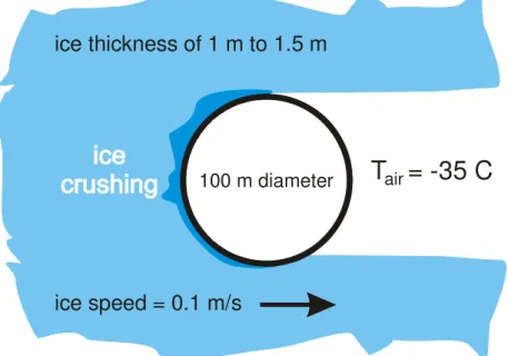
The first scenario was as follows: Estimate the loads that would be exerted on a 100 m wide
vertical caisson structure that is in moving pack ice. The ice thickness could range from 1.0 m to 1.5 m and the ice speeds are low (typically 0.1 m/s). Assume that the ice fails in crushing. Temperatures could be as low as -35°C.
Figure 1: Schematic illustration of the ice interaction with a vertical caisson structure (Scenario #1)
Anne Barker Approach
Anne used the expression on page 168 of the Standard to estimate these loads. She calculated a global pressure according to Equation (A.8-20)
(A.8-20) FG = pG h w
where FG is the global force, pG is the global ice pressure, h is the ice thickness and w is the structure width. The ice pressure was calculated using Equation (A.8-21) as
(A.8-21) pG = CR (h/h1)n (w/h)m
where pG is the global average ice pressure in MPa, w is the projected width of the structure in m, h is the thickness of the ice sheet in m, h1 is a reference thickness of 1 m, m is an empirical coefficient equal to −0.16, n is an empirical coefficient, equal to −0.50 + h/5 for h < 1.0 m,
ice thickness of 1 m to 1.5 m
ice speed = 0.1 m/s
T = -35 C
air 100 m diameterand to −0.30 for h ≥ 1.0 m, and CR is the ice strength coefficient, expressed in MPa. The Standard gives information on the CRvalue and suggests using a value of 2.8 for Beaufort Sea ice and 1.8 for Baltic ice conditions. Anne checked the requirement that the aspect ratio (w/h) was greater than two so this equation would apply. Since the ice thickness was greater than 1 m, Anne used n=-0.3 and she assumed that this was Beaufort Sea ice based on the low temperature. This gave load values of 134 MN and 190 MN for h = 1.0 m and 1.5 m respectively. Anne indicated that a more accurate CR value could be determined, but the available information specified in the scenario was insufficient to do so.
Scott Baker Approach
Scott started by going to Section A8.2.4.3 which describes vertical structures. He then read the section on the failure modes (A.8.2.4.2) to learn about the ice crushing failure mode. He started with the basic equation (A.8-19) for the global ice action FG with respect to the ice pressure and area:
(A.8-19) FG = pG AN
where pG is the ice pressure averaged over the nominal contact area associated with the global action and AN is the nominal contact area. Then, he used Equation A.8-21 to calculate the global average pressure using the same approach as that described above for Anne. His predicted load values were the same as those predicted by Anne.
Full-Scale Data
With respect to full-scale data, there were a number of ice loading events measured on the Molikpaq with similar ice conditions. Timco and Johnston (2004) outlined the loads on various caisson structures in the Beaufort Sea. From this data, a number of data points can be extracted that were described as ice crushing. These load values were measured with ice moving at a rate ranging from 0.04 to 0.4 cm/s with air temperatures that ranged from -12°C to -27°C. Some events had floating rubble around the Molikpaq but crushing was still noted as the failure mode for the ice. Thus these conditions are very similar to those developed for Scenario #1.
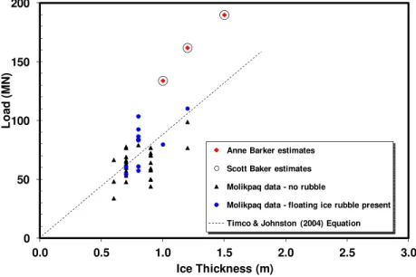
Figure 2 shows a plot of the measured load extrapolated to a 100 m wide structure. Measured values ranged up to 110 MN for an ice thickness of 1.2 m. There is a trend of increasing load with increasing ice thickness.
Timco and Johnston (2004) developed predictive equations for ice loads on vertical caisson structures. The loads were a function of the failure mode of the ice. For ice crushing, the load equation is FG = Tf w h where Tf is a failure mode parameter which is 1.09 MN/m2 for ice crushing and w is the caisson width and h is the ice thickness. This curve is also plotted on Figure 2. It should be noted that the full-scale values in Figure 2 and the Timco and Johnston (2004) equation relate to measured ice load values. Therefore they are not upper bound values.
Bob Frederking Comments
In any application of a standard it is advisable to go back and review the objectives of the standard. In the Scope of ISO 19906 it states “The objective of this International Standard is to ensure that offshore structures in arctic and cold regions provide an appropriate level of reliability with respect to personnel safety, environmental protection and asset value to the owner, to the industry and to society in general.” Thus it is a reliability based standard, in
which either probabilistic or deterministic methods may be used. In either method an equation for calculating ice forces is required, and this is what is being evaluated here. Equation A.8-21 is a fairly simple equation; ice thickness and structure width are given, only the ice strength coefficient CR is open to interpretation. Anne has used the information that the air temperature could be as low as -35 °C to take a value of 2.8 MPa for CR. She has also assessed the limit of applicability of Equation A.8-21 to cases of aspect ratio (width/ice thickness) greater than 2. Scott, not being familiar with 19906, went back and reviewed both A.8.2.4.2 Ice failure modes and A.8.2.4.3 Vertical structures. He then applied Equation A.8-21 and determined the same values of global ice actions as Anne.
Figure 2: Load comparisons for Scenario #1
As indicated in clause A.8.2.4.3.3 Global pressure for sea ice, Equation A.8-21 was intended to provide an upper bound to global ice pressure. Thus it is not surprising that the predicted loads are in agreement with the full-scale data but slightly higher than individual load measurements. In clause A.8.2.4.3.3, structure rigidity is mentioned and that in certain circumstances the degree of rigidity could increase or decrease the value of CR. This issue is discussed extensively in A.8.2.4.3.3, so it is surprising that neither mentioned this. The next clause, A.8.2.4.3.4 Influence of local ice conditions on ice pressures, provides guidance on how CR could be adjusted to local ice conditions. The intention in clauses A.8.2.4.3.3 and A.8.2.4.3.4 was to provide guidance so that appropriate values of CR could be determined for ice conditions other that the Beaufort or Baltic Seas. Anne commented that the available information specified in the scenario was insufficient to determine a more accurate CR value.
SCENARIO #2 – MULTI-LEG PLATFORM
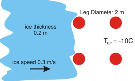
The second scenario was as follows: Estimate the loads on the front legs of 4-legged multi-leg
platform in mild ice conditions. The width of the leg is 2 m and the ice is 0.2 m thick. The ice advances in a direction perpendicular to the line between the two legs at a speed of 0.3 m/s. The air temperature is moderate (say -10°C). Estimate the loads on each leg and comment on the non-simultaneity of the loads on the legs (i.e. will doubling the load on one leg give an accurate estimate of the total load on the platform?). What factors should influence the loads?
0 50 100 150 200 0.0 0.5 1.0 1.5 2.0 2.5 3.0 Lo a d ( M N ) Ice Thickness (m)
Anne Barker estimates Scott Baker estimates Molikpaq data - no rubble
Molikpaq data - floating ice rubble present Timco & Johnston (2004) Equation
Figure 3: Schematic illustration of ice interacting with a multi-leg platform (Scenario #2).
Anne Barker Approach
Anne used Equation (A.8-60) to estimate the global action Fs as: (A.8-60) FS = ks kn kj F1
where F1 is the action on one leg, ks accounts for the interference and sheltering effects, kn accounts for the effect of non-simultaneous failure, and kj accounts for ice jamming. She did not use the value of the ice speed nor the temperature in the calculations. Since the spacing between the legs was not given, she assumed a value of 30 m. The values used in Equation A8-60 were determined as follows:
• ks= 3.5 (assumed maximal sheltering given 90° loading);
• kn = 0.9 (non-simultaneous but assumed that simultaneous failure not likely unless the structure was very compliant – didn’t know from the data provided);
• kj = 1 (jamming not expected since L/w >4. No guidance was given for the value so a value of 1 was assumed)
• F1 was calculated using Equation A.8-21 (given above). For this calculation, m =-0.16,
n =-0.46 (since h<1 m) and CR was taken as 2.8. (Anne commented that more
information on estimating the CR value would be useful). This gave pG of 4.1 MPa and a value for F1 of 1.6 MN. An assumption was made that the ice would fail in crushing. Then the global action would be FS = 3.5*0.9*1*1.6 = 5 MN.
Scott Baker Approach
Scott also used Equation A.8-60 to determine the global action on the platform. He started by determining the action on one leg using information in section A.8.2.4.3. He used Equation A.8-21 to first determine the pressure pG on the leg. Based on the text on page 169, he used a value for CR of 1.8 since the ice speed was greater than 0.1 m/s. He determined a value for pG of 2.61 MPa. Based on this and Equation A.8-20 he calculated the action on one leg as 1.04 MN.
He determined the coefficients for Equation A.8-60 based on the following reasoning:
Leg Diameter 2 m
ice thickness
0.2 m
ice speed 0.3 m/s
• ks – the sheltering factor. Based on the text on page 178 for a typical multi-leg platform with four legs, the maximal sheltering factor is 3.0 to 3.5. He chose a value of 3.5 as a conservative value;
• kn – the effect of non-simultaneous failure – here he assumed a value of 0.9 based on information on page 178 and noted that there was no other choice;
• ks – the effect of jamming – using the information on page 178 ice jamming is expected if L/w <4. Since the clear distance between the legs (L) was not given, he assumed a value of 10 m. Thus L/w = 5 so jamming would not be expected. Scott noted that the Standard does not provide further details for kj so he assumed a value of 1 for the calculations.
Scott used Equation A.8-60 and these values to determine the global action of (3.5*0.9*1*1.04) = 3.3 MN.
He commented that there was very little information on kn so he couldn’t comment on the non-simultaneity of the loads.
Local Pressure Analysis
Garry decided to look at the approach for the local design pressure. He did this since the ice-loaded area was quite small (0.4 m2) which is typically associated with areas for local pressures. He used the ISO Section A.8.2.5.2 Local actions from thin first-year ice and specifically Section A.8.2.5.2.3 Full thickness local pressure to estimate the full thickness ice pressure (pF) as
(A.8-63) pF = 4.0 for h ≤ 0.35 m
Then, in a deterministic design the ISO code states that the local pressure (pL) acting on the loaded area (which is given by Equation A8.61 viz., A = a wL where a is the height of the loaded area and wL is the width of the loaded area) is given by
(A.8-64) pL = γL pF
where γL = 2.5. Thus this gave a local pressure of 10 MPa. To determine an estimate of the
force for this calculation, the area is required. Here the code states that the loaded area in this case is a*wL and it is illustrated in Figure A8-18. This figure illustrates that the loaded height is 40% of the full ice thickness (i.e., a/h = 0.4). Thus, the force on the leg, assuming a width of 2 m is given by FL = γL pF (0.4 h) w = 2.5*4*0.4*.2*2 = 1.6 MN. This is the same global
force calculated by Anne using the global load approach.
It is interesting to note that this value of 1.6 MN could easily be obtained by multiplying the
pF value by the ice thickness and the width of the leg, i.e, FL = pF * h*w = 4*.2*2 = 1.6 MN. Thus the code appears to get this value in an apparently more complicated manner (since the multiplication of the γL value of 2.5 and the 0.4 of the ice thickness results in a value of one).
A better explanation for this would be desirable.
Section A8.2.5.2.3 also potentially could cause mistakes since the first sentence reads that this local pressure is “associated with the full ice sheet (floe) thickness”. Thus one might imply that the whole ice thickness should be used for the loaded area calculation (instead of the 0.4 reduction). This is re-enforced by the definition of “a” in Equation A8.61 which states that a is the height of the loaded area. A logical assumption is that the loaded area is the ice
thickness. These potential mistakes could be avoided if a better explanation of Figure A8-18 was supplied for non-specialists of pressure-area jargon. That is, the code is not incorrect but a better explanation with regard to the use of Figure A8-18 would be useful.
Full-Scale Data
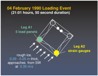
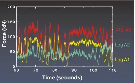
Johnston et al. (2000) reported on the loads measured on two legs of the Chinese JZ-20 platform. In this case, two legs were instrumented to measure the loads that result from advancing sea ice floes. One leg was equipped with five load panels, which allowed the local load and total leg load to be determined. The other leg was strain-gauged, providing another estimate of the leg load. Johnston et al. (2000) analyzed in detail an ice loading event that took place on the platform on February 4, 1990. During this event, rough ice with a thickness of 0.20 to 0.25 m thickness approached the platform from the SW at a speed of 0.35 m/s (see Figure 4). Leg A1 was fitted with five HSVA load panels and with this modification, the width of the leg was 2.02 m. Leg A2 was strain gauged and had a width of 1.67 m. Thus, these conditions are very similar to those developed for Scenario #2.
Figure 4: Details of the ice loading event on the Chinese JZ-20 platform (after Johnston et al. 2000).
More than 80 minutes of digital data is available for analysis. Johnston et al. (2000) selected a short 50 second interval for a detailed analysis. The event was chosen from the load record because it provided a good illustration of the transition from high-frequency loading to low-frequency, large oscillation, saw-tooth loading.
Figure 5 shows the load-time record for the ice loading event. The loads on both legs were quite cyclic with a change in frequency approximately half-way through the loading event. Loads on Leg A1 reached values of 100 kN (0.1 MN) whereas the loads on Leg A2 were lower and reached a value of approximately 80 kN (0.08 MN).
rough ice, thick, approaches from SW at 0.20 - 0.25 m 0.35 m/s Leg A2 strain gauges Leg A1
04 February 1990 Loading Event
(21:01 hours, 50 second duration)
Figure 5: Load-time series for the loading event analyzed by Johnston et al. (2000).
Johnston et al. (2000) also examined the relationship of the loads on each leg compared to the total load on the two legs. They did this by adjusting the leg diameter of Leg A1 to a width of 1.67 m by a linear scaling of the width. Table 1 shows the 95th percentile and 99th percentile loads on Leg A1 (2*FA1_a), Leg A2 (2*FA2) and the total load on two legs (FA1A2_a). Doubling
the load on Leg A1 results in an over-prediction of 28 - 30% for loads in the tail of the distribution. Extrapolation of the loads on Leg A2 over-predicts the measured total load on two legs by 11 - 18 %.
Table 1: Comparison of Extrapolated and Measured Loads in the Extreme Tail of the Distribution (after Johnston et al. 2000)
Table 2 provides a comparison of the predicted values with those measured on the JZ20 platform. The table provides a comparison of the predicted values both for a single leg and for the whole platform. Here the local load value calculated by Garry using the local pressure approach has been included for this comparison. The table shows disagreement in the predicted loads and a very significant difference between the measured and predicted loads.
Table 2: Comparison of the predicted and measured loads on the multi-leg platform
Time (seconds)
Force (
k
N
)
Leg A1 Leg A2 A1& A2Description Parameter 95th percentile 99th percentile
(kN) (kN)
Doubled, measured load on Leg A1 (adjusted) 2*FA1_a 156 167
Doubled, measured load on Leg A2 2*FA2 133 154
Total load on Leg A1 and Leg A2 FA1A2_a 120 130
AB global approach GT local pressure approach SB global approach JZ20 data
MN MN MN MN
Load on one 2 m wide leg 1.6 1.6 1.04 0.1
Bob Frederking Comments
The guidance in clause A.8.2.4.9 Multi-leg structures, is not complete and the additional guidance in the two references cited in the clause adds little. An estimate of the global ice action on a multi-leg structure requires assumptions and judgements. Equation A.8-60 for the global action requires the global action on a single leg, which is then adjusted by accounting for factors of sheltering, non-simultaneity and jamming between the legs. Both Anne and Scott used Equation A.8-21 to calculate the global ice action on one leg. Leg diameter and ice thickness are given, so again the strength coefficient CR is open to interpretation. Scott used the Baltic Sea CR as being representative of the ice conditions for Scenario #2. The fact that Anne used the Beaufort Sea value of CR, but expressed uncertainty in estimating values of CR suggests that clearer guidance could be provided in clause A.8.2.4.3.3.
Determining the global action on the multi-leg structure requires estimating values of the sheltering factor, ks, and the non-simultaneity, kn, factor. Guidance is provided for these values, based on limited field measurements and physical model tests. The jamming factor kj is perhaps misleading, since if jamming occurs, the ice action on a single leg is no longer germane, and ice action on a blocked structure should be considered. This is an area that could be improved in the next edition of ISO 19906.
Comparing the predicted actions with the results of full-scale measurements from JZ-20 structure in the Bohai Sea is perhaps misleading. The thin, and consequently warm ice, even for an air temperature of –10°C would imply a CR value less than 1.8 MPa. Furthermore, the JZ-20 measurements were only on two legs. Some allowance should be made for ice actions on all 4 legs. But even allowing for this the predicted loads are more than an order of magnitude larger than the loads measured on the JZ20 platform.
Garry has examined local pressures as guided by clause A.8.2.5.3 to determine the local pressure and then the global force because the ice was thin and the global area was small (0.4 m2). Global ice pressure and local ice pressure are defined separately in the standard and are used for different purposes. Clause A.8.2.5 Local ice actions, introduces local pressures and points out that their application is for the design of local structure, that is the shell or stiffening elements. Local pressures are on local areas within a global area. Applying local pressures to determine a global force is not the intent of this group of clauses. As Garry pointed out A.8.2.5.3 seems to go through a circular argument of first reducing the thickness (multiplying by a factor of 0.4) and then increasing the local pressure by a factor of 2.5. This does incidentally produce the same global force, but the important and intended result of this process is to specify realistic local ice pressures on small areas, which are required in the safe design of local structure.
In general, in using any standard it is important to read the document more broadly than just the section of interest. Thought, care and no small amount of time go into organizing content and selecting wording to guide an engineer to a safe design. Having fresh eyes use a standard and provide feedback is welcomed by standards developers, and does lead to improvement. DISCUSSION AND CONCLUSIONS
This simple approach has identified a number of interesting features about the ISO Arctic offshore structures standard.
The scenario of predicting loads on a wide vertical caisson was relatively straightforward and the predicted load values by both predictors agreed and were in line with observed full-scale data. Both predictors commented that they would like to have a way to refine the Ice Strength coefficient CR to improve the accuracy of the predictions for different locations. Anne listed more assumptions for her calculations (i.e. she assumed no ridges, no structural compliance) which were not noted by the engineer with no ice mechanics experience. Scott commented “In
general, calculating the global action due to ice crushing (Eqn A.8-20) was fairly straightforward, with the only real issue being to determine the appropriate CR value.”
The multi-leg scenario was not as straightforward as the simple vertical caisson. Anne and Scott both used the same approach but they predicted different values due to different assumptions. None of the predictions were even close to the observed full-scale data. Anne noted more insight by indicating that there are several influencing factors including the ice drift angle, jamming, non-simultaneous loading, structural compliance, leg spacing influences) which were not evident to Scott in a straightforward calculation. Both predictors commented that the guidance on the “k” factors in Equation A.8-60 was very sparse. Both would have liked more guidance on all of these factors (i.e. ks, kn and kj). Both predictors made similar comments about the lack of a methodology to refine the value of CR. Of course the fact that the predicted loads were not close to the full-scale values must be addressed in a revised version of the Standard. Garry’s additional calculation to look at local pressures provided some interesting results and highlighted the need to distinguish between the local pressure and the global pressure. Bob’s comments with respect to this are particularly important in this regard.
This paper has presented a simple methodology to evaluate some aspects of the ISO Arctic offshore structures Standard. Two simple scenarios were developed and some insight into the use and limitations of the Standard were outlined. Scott summarized his experience as follows: “Overall the code is relatively well laid out and not too hard to follow for someone
who’s inexperienced with it. As we discussed, it would be valuable to include one or more sample calculations for common problems”.
This exercise has pointed out the absolute need to read the code thoroughly and more broadly than just what appears to be the section of interest. Engineers with ice mechanics experience were much more aware of the assumptions and limitations of the standard compared to an experienced engineer with limited ice knowledge. Even with these relatively basic scenarios, there was some disagreement in the estimated loads. Ongoing use and dialogue about the ISO 19906 Arctic offshore structures standard should help to improve the standard and highlight its strengths and weaknesses.
REFERENCES
Blanchet, D., Croasdale, K.R., Spring, W., Thomas, G. 2007. ISO/TC 67/SC7/WG 8 - An International Standard for Arctic Offshore Structures. Proceedings POAC'07, Vol. 1, pp 3-20, Dalian, China.
ISO 19906, 2010. Petroleum and natural gas industries-Arctic offshore structures. International Organization for Standardization. Geneva, Switzerland.
Johnston, M.E., Timco, G.W., Frederking, R., Jochmann, P. 2000. Simultaneity of Measured Ice Load on Two Legs of A Multi-Leg Platform. Proceedings OMAE’00, Paper 00-1007, New Orleans, USA.
McKenna, R., Spring, W., Thomas, G., 2011. Use of the ISO 19906 Arctic Structures Standard. Proceedings OTC Arctic Technology Conference, Paper OTC 22074, Houston, TX, USA.
Masterson, D.M., Tibbo, J.S. 2011. Comparison of ice load calculations using ISO 19906, CSA, API and SNIP. Proceedings POAC'11, paper POAC11-59, Montreal, QC, Canada. Määttänen, M., Kärnä, T., 2011. ISO 19906 ice crushing load design extension for narrow structures. Proceedings POAC'11, paper POAC11-63, Montreal, QC, Canada.
Moslet, P.O., Gudmestad, O.T., Sildnes, T., Sæbø, E. 2011. The new ISO 19906 standard and related Arctic activities at DNV. Proceedings POAC'11, paper POAC11-62, Montreal, QC, Canada.
OGP, 2010. Calibration of action factors for ISO 19906 Arctic offshore structures. Report No. 422, International Association of Oil & Gas Producers, December 2010.
Palmer, A.C., 2011. Moving on from ISO 19906: what ought to follow? Proceedings POAC'11, paper POAC11-60, Montreal, QC, Canada.
Spring, W., McKenna, R.F., Thomas, G., Blanchet, D. 2011. ISO 19906 - an international standard for arctic offshore structures. Proceedings POAC'11, paper POAC11-K3, Montreal, QC, Canada.
Thomas, G., Masterson, D., Spring, W. 2011. Overview of Case Studies for Draft ISO 19906. Proceedings OTC Arctic Technology Conference, Paper OTC 22073, Houston, TX, USA. Timco, G.W., Johnston, M. 2004. Ice Loads on the Caisson Structures in the Canadian Beaufort Sea. Cold Regions Science and Technology 38, 185-209.