Expectation propagation in GenSpace graphs for summarization

Publisher’s version / Version de l'éditeur:

Questions? Contact the NRC Publications Archive team at https://publications-cnrc.canada.ca/fra/droits

L’accès à ce site Web et l’utilisation de son contenu sont assujettis aux conditions présentées dans le site LISEZ CES CONDITIONS ATTENTIVEMENT AVANT D’UTILISER CE SITE WEB.

The 9th International Conference on Data Warehousing and Knowledge

Discovery (DaWak 2007) [Proceedings], 2007

READ THESE TERMS AND CONDITIONS CAREFULLY BEFORE USING THIS WEBSITE. https://nrc-publications.canada.ca/eng/copyright

NRC Publications Archive Record / Notice des Archives des publications du CNRC :

https://nrc-publications.canada.ca/eng/view/object/?id=bb62158f-31f2-4eda-9389-61f7c572a050 https://publications-cnrc.canada.ca/fra/voir/objet/?id=bb62158f-31f2-4eda-9389-61f7c572a050

NRC Publications Archive

Archives des publications du CNRC

This publication could be one of several versions: author’s original, accepted manuscript or the publisher’s version. / La version de cette publication peut être l’une des suivantes : la version prépublication de l’auteur, la version acceptée du manuscrit ou la version de l’éditeur.

Access and use of this website and the material on it are subject to the Terms and Conditions set forth at

Expectation propagation in GenSpace graphs for summarization

Geng, Liqiang; Hamilton, Howard J.; Korba, Larry

Expectation Propagation in GenSpace

Graphs for Summarization*

Geng, L., Hamilton, H.J., and Korba, L.

September 2007

* The 9th International Conference on Data Warehousing and Knowledge Discovery (DaWak 2007). September 2007. NRC 49355.

Copyright 2007 by

National Research Council of Canada

Permission is granted to quote short excerpts and to reproduce figures and tables from this report, provided that the source of such material is fully acknowledged.

Expectation Propagation in GenSpace Graphs for

Summarization

Liqiang Geng1, Howard J. Hamilton2, and Larry Korba1

1

Information Security Group, NRC-IIT, Fredericton, NB, E3B 9W4 2

Department of Computer Science, University of Regina, Regina, SK, S4S 0A2 1

Information Security Group, NRC-IIT, Ottawa, ON, K1A 0R6

[email protected], [email protected], [email protected]

Abstract. Summary mining aims to find interesting summaries for a data set and to use data mining techniques to improve the functionality of Online Analytical Processing (OLAP) systems. In this paper, we propose an interactive summary mining approach, called GenSpace summary mining, to find the interesting summaries based on user expectations. In the mining process, to record the user’s evolving knowledge, the system needs to update and propagate new expectations. In this paper, we propose a linear method for consistently and efficiently propagating user expectations in a GenSpace graph. For a GenSpace graph where uninteresting nodes can be marked by the user before the mining process, we propose a greedy algorithm to determine the propagation paths in a GenSpace subgraph that reduces the time cost subject to a fixed amount of space.

1 Introduction

Summarization at different concept levels is a crucial task addressed by online analytical

processing (OLAP). For a multidimensional table, the number of OLAP data cubes is exponential. Exploiting the cube space to find interesting summaries with basic rollup and drilldown operators is a tedious task for users. Many methods and tools have been proposed to facilitate the exploitation process. The use of iceberg cube has been proposed to selectively aggregate summaries with an aggregate value above minimum support thresholds [1]. This approach assumes that only the summaries with high aggregate values are interesting. Discovery-driven exploration has been proposed to guide the exploitation process by providing users with interestingness measures based on statistical models [9]. The use of the diff operator has been proposed to automatically find the underlying reason (the detailed data that accounts for the difference) for a surprising difference in a data cube identified by the user [8].

Nonetheless, these approaches for finding interesting summaries have three weaknesses. First, huge amount of summaries can be produced, and during exploration, the data analyst must examine summaries one by one to assess them before the tools can be used to assist the exploitation. Secondly, the capacity for incorporating existing knowledge is limited. Thirdly, the ability to respond to dynamic changes in the user's

knowledge during the knowledge discovery process is limited. For example, if the information that more Pay-TV shows are watched during the evening than the afternoon has already been presented to the user, it will subsequently be less interesting to the user to learn that more Pay-TV shows are watched starting at 8:00PM than shows starting at 4:00PM

To overcome these limitations, we are developing a summarization method based on generalization space (GenSpace) graphs [3]. The GenSpace mining process has four steps [3]. First, a domain generalization graph (DGG) for each attribute is created by explicitly identifying the domains appropriate to the relevant levels of granularity and the mappings between the values in these domains. The expectations are specified by the user for some nodes in each DGG to form an ExGen graph and then propagated to all the other nodes in the ExGen graph. In this paper, the term “expectations” refers to the user’s current beliefs about the expected probability distributions for a group of variables at certain conceptual levels. Second, the framework of the GenSpace graph is generated based on the ExGen graphs for individual attributes, and the potentially interesting nodes in this graph are materialized. Third, the given expectations are propagated throughout the GenSpace subgraph consisting of potentially interesting nodes, and the interestingness measures for these nodes are calculated [5]. Fourth, the highest ranked summaries are displayed. Expectations in the GenSpace graph are then adjusted and the steps are repeated as necessary. Having proposed the broad framework for mining interesting summaries in GenSpace graphs in [3], we now propose a linear expectation propagation method that can efficiently and consistently propagate the expectations in GenSpace graphs.

Significant work has been conducted on incorporating user’s domain knowledge and applying subjective interestingness measures to find interesting patterns. However, all of these methods only apply to discovered rules. In this paper, we incorporate the user’s knowledge to find interesting summaries.

Expectation propagation in GenSpace is similar to Bayesian belief updating in that they both propagate a user’s beliefs or expectations from one domain to another. However, the Bayesian belief updating deals with conditional probability of different variables, and does not deal with multiple concept levels of a single variable. Therefore, it does not apply to the problem addressed in this paper.

The remainder of this paper is organized as follows. In Section 2, we give the theoretical basis for ExGen graphs and GenSpace graphs. In Section 3, we propose a linear expectation propagation method. In Section 4, we propose a strategy for selecting propagation paths in a GenSpace subgraph. In Section 5, we explain our experimental procedure and present the results obtained on Saskatchewan weather data. In Section 6, we present our conclusions.

2 ExGen Graphs and GenSpace Graphs

An ExGen graph is used to represent the user’s knowledge relevant to generalization for an attribute, while a GenSpace graph is used for multiple attributes. First, we give some formal definitions.

Definition 1. Given a set X = {x1, x2, …, xn} representing the domain of some attribute and

a set P = {P1, P2, …, Pm} of partitions of the set X, we define a nonempty binary relation

p

p

Pi, there exists a section Sb ∈ Pj, such that Sa ⊆ Sb . For convenience, we often refer to the

sections by labels. The graph determined by generalization relation is called domain

generalization graph (DGG). Each arc corresponds to a generalization relation, which is a

mapping from the values in the parent node to that of the child. The bottom node of the graph corresponds to the original domain of values X and the top node T corresponds to the most general domain of values, which contains only the value ANY.

In the rest of the paper, we use “summary”, “node”, and “partition” interchangeably.

Example 1. Let MMDDMAN be a domain of morning, afternoon, and night of a specific non-leap year {Morning of January 1, Afternoon of January 1, Night of January 1, …,

Night of December 31}, and P a set of partitions {MMDD, MM, Week, MAN}, where MMDD = {January 1, January 2, …, December 31}, MM = {January, February, …, December}, Week = {Sunday, Monday, …, Saturday}, and MAN = {Morning, Afternoon, Night}. Values of MMDDMAN are assigned to the values of the partitions in the obvious

way, i.e., all MMDDMAN values that occur on Sunday are assigned to the Sunday value of

Week, etc. Here MMDD

p

p

from the generalization relation.

Definition 2. An expected distribution domain generalization (or ExGen) graph

〉

〈P, Arc ,E is a DGG that has expectations associated with every node. Expectations represent the expected probability distribution of occurrence of the values in the domain corresponding to the node. For a node (i.e., partition) Pj = {S1, …, Sk}, we have

1 ) ( 0 , ≤ ≤ ∈ ∀S_i P_j E S_i and ( ) 1 1 =

∑

E , where E(Si) denotes the expectation of

occurrence of section Si.

Example 2. Continuing Example 1, for the partition MAN = {Morning, Afternoon, Night}, we associate the expectations [0.2, 0.5, 0.3], i.e., E(Morning) = 0.2, E(Afternoon) = 0.5, and E(Night) = 0.3.

Figure 1. An Example DGG.

Definition 3. Assume node Q is a parent of node R in an ExGen graph, and therefore for each section Sb ∈ R, there exists a set of specific sections {

k a a

S

S

,

...,

U

∑

( , we say that nodes Q and R are

consistent. An ExGen graph G is consistent if all pairs of adjacent nodes in G are

consistent.

Theorem 1. An ExGen graph G is consistent iff every node in G is consistent with the bottom node.

Proof. The proof of Theorem 1 is given in [2].

An ExGen graph is based on one attribute. If the generalization space consists of more than one attribute, we can extend it to a GenSpace graph [2]. Each node in a GenSpace is the Cartesian product of nodes in all ExGen graphs. Theorem 1 for ExGen graphs can be adapted directly to GenSpace graphs.

3 Propagation of Expectations in GenSpace Graphs

Due to the combinational number of the nodes in a GenSpace graph, it is not practical to require that the user specify the expectations for all nodes. In exploratory data mining, the user may begin with very little knowledge about the domain, perhaps only vague assumptions about the (a priori) probabilities of the possible values at some level of granularity. After the user specifies these expectations, a data mining system should be able to create default preliminary distributions for the other nodes. We call the problem of propagating a user’s expectations from one node or a group of nodes to all other nodes in a GenSpace graph the expectation propagation problem.

For each node in a GenSpace graph, the user can specify the expectations as an explicit probability distribution, or as a parameterized standard distribution, or leave the expectations unconstrained. If a standard distribution is specified, it is discretized into an explicit probability distribution. If expectations are not specified for a node, they are obtained by expectation propagation.

We propose the following three expectation propagation principles: (1) the results of propagations should be consistent, (2) if new expectations are being added, the new information should be preserved, while the old expectations should be changed as little as possible, and (3) if available information does not fully constrain the distribution at a node, the distribution should be made as even as possible.

To guarantee that propagation preserves consistency, we first propagate the new expectations directly to the bottom node, and then propagate the expectations up to the entire graph. Since bottom-up propagation makes all nodes consistent with the bottom node, the entire graph is consistent, according to Theorem 1. Bottom-up propagation will be elaborated in Section 4. Here we concentrate on the first step of our approach, specific

expectations determination, i.e., how to propagate expectations from any non-bottom

nodes specified by the user to the bottom node.

Based on expectation propagation principles, we treat the problem of specific expectations determination as an optimization problem. Given a set of nodes with new expectations, the expectations at the bottom node X are found by representing the constraint due to each node as an equation and then solving the set of equations. For a

node i with ji sections Sik, where 1≤k ≤ ji, assume that E’(Sik) is the new expectation

for each section Sik, and s is an element of X, i.e., s ∈ X. We have '( ) '( _ik) S s S E s E ik =

∑

Under these constraints, we minimize 2

)) ( ) ( ' (

∑

E , where E’(s) and E(s) are

new and old expectations for element s in bottom node, to make the changes to the node X as small as possible. This minimization reflects the intuition that the old knowledge is preserved as much as possible. Since the number of variables equals to the number of the records in the bottom node, for large GenSpace graphs, the optimization process, like Lagrange multipliers, has a prohibitive time and space cost.

We propose the linear propagation method for finding an approximation to the solution to the optimization problem. We use the following linear equation to obtain the new expectations for the bottom node,

) ( ) ( ) ( ' ) ( ' E s S E S E s E ik ik

= , where s is a section of X and

s

∈

S

equation, we accept the probability ratio among the sections and also retain the ratio among the elements of each section.

This method has three advantages. First, it is computationally efficient, because it involves only linear computation with time complexity of O(|N||X|), where |N| is the size of node N where the user changed his/her expectations. Secondly, it does not need to resolve conflicts among the user’s new expectations, because we propagate new expectations in sequence rather than simultaneously as with the optimization method. Thirdly, we have identified an upper bound in terms of the changes of expectations specified by the user for the expectation changes between the old and new expectations for all the nodes in a GenSpace graph. In this sense, the user’s old information is preserved.

Theorem 2. Let N be a node in a GenSpace graph G with m sections S1, ..., Sm. Suppose

the old expectations for node N are {E(S1), …, E(Sm)}, the new expectations for N are )} ( ' ..., ), ( ' {E S₁ E S_m and − _{= α} = _{( )} ) | ) ( ) ( ' | ( max 1 i i i m i _{E S} S E S E _{. After propagating}

E’ from N to the entire GenSpace graph using the linear propagation method, the relative

variance vP for any node P satisfy =

∑

= P m i iP iP iP P P S E S E S E m v 1 2 ) ) ( ) ( ) ( ' ( 1 _{, where}

mP denotes the number of sections in node P.

Proof: the proof is given in the Appendix.

Example 3. Theorem 2 tells us that if we change the expectations for each weekday by no more than 20%, after propagation, the expectation change for all other nodes (including nodes Month, Day and, Morning-Afternoon-Night) will not exceed 20%.

A drawback of the linear propagation method is that if expectations in two or more nodes are updated simultaneously, it cannot update expectations in other nodes

simultaneously, as the optimization method does. However, we can obtain an approximation by applying the linear method multiple times, once for each updated node.

4 Propagation in GenSpace Subgraphs

If the user can identify some uninteresting nodes, we can prune them before propagation and only materialize the potentially interesting nodes. Pruning all uninteresting nodes saves the most storage, but it may increase propagation time.

Selecting views to materialize draws much attention from researchers [4, 6, 7]. Harinarayan et al. proposed a linear time cost model for aggregating a table [4]. They found that the time cost for producing a summarization is directly proportional to the size of the raw table. Therefore, in our case, when we propagate expectations from node A to node B, the time cost is directly proportional to the size of node A.

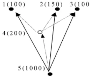
Example 4. In Figure 2, nodes are shown with a unique identifier and their size. The solid ovals denote interesting nodes and the blank ovals denote uninteresting nodes. If we prune node N4, the propagation cost from node N5 to N1, N2, and N3 is size(N5) * 3 = 3000. If we

preserve N4 as a hidden node, the propagation cost is size(N5) + size(N4) * 3 = 1600.

Keeping hidden nodes reduces the propagation cost by nearly 50%.

1 ( 1 0 0 ) 2 ( 1 5 0 ) 3 ( 1 0 0 )

4 ( 2 0 0 )

5 ( 1 0 0 0 )

Figure 2. Efficiency Improvement Due to Keeping Uninteresting Nodes.

Sarawagi et al. encountered a similar problem when they calculated a collection of group-bys [10]. They converted the problem into a directed Steiner tree problem, which is an NP-complete problem. They used a heuristic method to solve their problem. Here, we consider our problem as a constrained directed Steiner tree problem, where there is a space limit for the uninteresting nodes. Furthermore, to use a Steiner tree model, we need to create additional arcs in the graph to connect all pairs of nodes that have a generalization relation, which causes extra storage space. We propose a greedy method to select hidden nodes and find an efficient propagation path for subgraphs.

Definition 4. (Optimal Tree) Given a GenSpace graph G = <P, Arc, E> and a set of nodes N ⊆ P such that the bottom node X ∈ N, a optimal tree OT of N in G is a tree that consists of nodes in N. The root of the tree is X. For every non-bottom node n ∈ N, its parent is an ancestor in G of minimum size that belongs to N.

An optimal tree for a set of nodes has the most efficient propagation paths for the subgraph consisting of these nodes, because every node obtains expectations from its smallest possible ancestor in the subgraph.

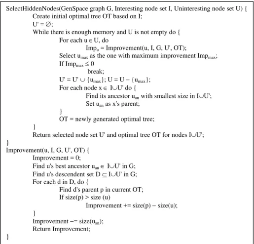
Algorithm SelectHiddenNodes for choosing hidden nodes and determining the propagation paths is given in Figure 3. We first create the optimal tree consisting of only the interesting nodes, then check the uninteresting nodes, and select the one that results in the greatest reduction in the scanning cost, which is defined as the sum of the sizes of the parent nodes in the optimal trees for all nodes. Then we modify the optimal tree to incorporate the selected nodes. This process continues until the space cost reaches the given threshold or no improvement can be obtained or no candidate uninteresting nodes are left. Selecting an uninteresting node will affect propagation efficiency in two ways. First it will cause an extra propagation cost for propagating expectations to this node; secondly, it may reduce the cost for its interesting descendents. Function Improvement calculates the efficiency improvement for an uninteresting node u. If it returns a positive value, it will reduce the scanning cost.

Figure 3. Algorithm for Selecting Hidden Nodes and Creating Optimal Tree. SelectHiddenNodes(GenSpace graph G, Interesting node set I, Uninteresting node set U) {

Create initial optimal tree OT based on I; U' = ∅;

While there is enough memory and U is not empty do { For each u ∈U, do

Impu = Improvement(u, I, G, U', OT);

Select umax as the one with maximum improvement Impmax; If Impmax ≤ 0

break;

U' = U' ∪ {umax}; U = U − {umax}; For each node x ∈ I∪U' do {

Find its ancestor uan with smallest size in I∪U'; Set uan as x's parent;

}

OT = newly generated optimal tree; }

Return selected node set U' and optimal tree OT for nodes I∪U'; }

Improvement(u, I, G, U', OT) { Improvement = 0;

Find u's best ancestor uan ∈ I∪U' in G; Find u's descendent set D ⊆ I∪U' in G; For each d in D, do {

Find d's parent p in current OT; If size(p) > size (u)

Improvement += size(p) − size(u); }

Improvement −= size(uan); Return Improvement; }

5 Experimental Results

We implemented the GenSpace summary mining software and applied it to three real dataset. Due to space limitations, we only present the results for Saskatchewan weather dataset here. This dataset has 211,584 tuples and four attributes, time, station,

temperature, and precipitation. Take reference to [2] for the ExGen graphs for these

attributes.

First, we compared the efficiency of the linear propagation method and the optimization method on the ExGen graph in Figure 1. The experiments were conducted in Matlab 6.1 in a PC with 512M memory and 1.7 GHz CPU. We tested on two cases. Table 1 compares the running time. We can see that for the optimization method, when the size of the bottom node (number of the variables) increases from 365 to 1095, the running time increases dramatically from 67 seconds to 1984 seconds. For the linear propagation method, in both cases, the running time is unperceivable.

Table 1. Comparison of running time between optimization and linear methods

Running time (Sec) Cases # of variables # of constraints

Optimization linear

Case 1 365 19 67 <1

Case 2 1095 3 1984 <1

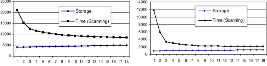
To show the efficiency of the SelectHiddenNodes algorithm, we present two cases: (1) mark all nodes in the lowest 5 levels (out of 19 levels) as uninteresting and (2) mark all the nodes in the lowest 5 levels or with specific date values or specific temperature values as uninteresting. The results are shown in Table 2. The Storage column lists the storage cost in thousands of records. The Scanning column lists the number of the records scanned during propagation, in thousands of records. The Time column lists the propagation cost in seconds. We first compare the storage and the scanning costs between the subgraph obtained from SelectHiddenNodes and that from pruning all uninteresting nodes.In case 1, after selecting hidden nodes, the storage increased by 25%, while the scanning cost decreased by 60%. In case 2, the storage cost increased by 26%, and the scanning cost decreased by 82%. In both cases, the scanning cost decreased significantly while the storage cost increased by a smaller percentage. Then we compare the storage and time costs between the subgraph selected by SelectHiddenNodes and the entire GenSpace graph. For both cases, both storage and scanning costs are significantly less for the subgraph obtained from SelectHiddenNodes. Figure 4 shows the storage and scanning costs after selecting varying numbers of nodes for cases 1 and 2. The X-axis denotes the number of the nodes currently selected, and the Y-axis denotes the storage and scanning costs, in thousands of records. We can see that in both cases, the first few nodes contribute the most to the reduction of the scanning cost.

We also tested the scalability of the algorithm. Figure 5(a) compares the scanning costs of propagation in the full GenSpace graph, the subgraph composed of only interesting

nodes, and the subgraph obtained from SelectHiddenNodes. Figure 5(b) compares the corresponding storage costs. The results show that the time savings are significant for

SelectHiddenNodes regardless of the size of the bottom nodes, and that its storage cost

falls in an acceptable range.

Table 2. Propagation Costs in GenSpace Subgraph.

Storage (K) Scanning (K) Time(Sec)

Entire GenSpace Preserve all 15309 18669 2037

Prune all 4128 21173 2149 Case 1 SelectHiddenNodes 5156 8391 1056 Prune all 912 11703 983 Case 2 SelectHiddenNodes 1152 2155 152

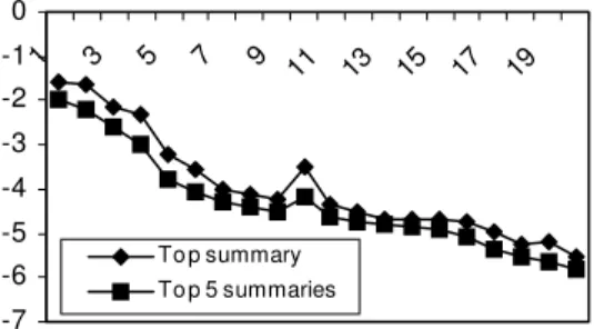
The analysis for the detailed process and the quality of the results was presented in [2]. In this paper, we show the interestingness values (logarithm of the variances) for the top summaries and the top five summaries for twenty iterations (see Figure 6). As the process iterates, both the measures are roughly decreasing functions of the number of iterations. This shows that the user’s expectations become closer to the real distributions, which coincides with our expectations and demonstrates the effectiveness of our method.

0 5000 10000 15000 20000 25000 1 2 3 4 5 6 7 8 9 10 11 12 13 14 15 16 17 18 Storage Time (Scanning) 0 2000 4000 6000 8000 10000 12000 14000 1 2 3 4 5 6 7 8 9 10 11 12 13 14 15 16 17 18 Storage Time (Scanning)

(a) Case 1 (b) Case 2

Figure 4. Change Trend of Storage and Time When Selecting Hidden Nodes.

0 2000 4000 6000 8000 10000 12000 14000 16000 40K 80K 120K 160K 200K Size of bottom nodes

T hous ands of r ec or ds s c a nned GenSpace Pruning all SelectHiddenNodes 0 2000 4000 6000 8000 10000 12000 40K 80K 120K 160K 200K Size of bottom nodes

T hous ands of r ec or ds s c a nned GenSpace Pruning all SelectHiddenNodes

Figure 5. Time saved in percentage for data sets with different sizes. -7 -6 -5 -4 -3 -2 -1 0 1 3 5 7 9 _{11 13 15 17 19} To p summary To p 5 summaries

Figure 6. Logarithm of variances for the top summaries in the first 20 iterations.

6 Conclusions

We proposed an efficient method to propagate a user’s expectations in a GenSpace graph, which describes a variety of ways of performing generalization. Based on the propagated expectations, the system finds interesting summaries in the GenSpace graph based on current expectations. We also proposed a strategy for selecting propagation paths in a GenSpace subgraph that reduces the time cost subject to a fixed amount of space. Experiments on real data sets show the effectiveness and efficiency of our approach. In the future, we will employ the known dependencies between attributes to facilitate the propagation process.

References

[1] Beyer, K. and Ramakrishnan, R., Bottom-up computation of sparse and iceberg CUBEs.

Proceedings of ACM SIGMOD, 359-370, 1999.

[2] Geng, L. and Hamilton, H. J., Expectation Propagation in ExGen Graphs for Summarization, Tech. Report CS-2003-03, Department of Computer Science, University of Regina, May 2003. [3] Hamilton, H. J., Geng, L., Findlater, L., and Randall, D. J., Efficient Spatio-Temporal Data

Mining with GenSpace Graphs, Journal of Applied Logic, 4(2):192-214, 2006.

[4] Harinarayan, V., Rajaraman, A., and Ullman, J. D., Implementing Data Cubes Efficiently.

Proceedings of ACM SIGMOD '96, 205-216, 1996.

[5] Hilderman, R.J. and Hamilton, H.J., Knowledge Discovery and Measures of Interest, Kluwer Acadamic, 2001.

[6] Lawrence, M. and Rau-Chaplin, A. Dynamic view selection for OLAP, Proceedings of

DaWaK2006 , Krakow, Poland, 33-44, September 4-8, 2006.

[7] Li, H., Huang, H., and Liu, S. PMC: Select materialized cells in data cubes, Proceedings of

DaWaK2005, 168-178, Copenhagen, Denmark, August 22-26, 2005.

[8] Sarawagi, S., Explaining Differences in Multidimensional Aggregates. In Proc. of the 25th Int'l

Conference on Very Large Databases (VLDB), 1999.

[9] Sarawagi, S., Agrawal, R., and Megiddo, N., Discovery Driven Exploration of OLAP Data Cubes. In Proc. Int. Conf. of Extending Database Technology (EDBT'98), March 1998.

[10] Sarawagi, S., Agrawal, R., and Gupta, A., On Computing the Data Cube. Research Report RJ10026, IBM Almaden Research Center, 1996.