HAL Id: hal-03026383
https://hal.inrae.fr/hal-03026383
Preprint submitted on 27 Nov 2020
HAL is a multi-disciplinary open access
archive for the deposit and dissemination of sci-entific research documents, whether they are pub-lished or not. The documents may come from teaching and research institutions in France or abroad, or from public or private research centers.
L’archive ouverte pluridisciplinaire HAL, est destinée au dépôt et à la diffusion de documents scientifiques de niveau recherche, publiés ou non, émanant des établissements d’enseignement et de recherche français ou étrangers, des laboratoires publics ou privés.
Distributed under a Creative Commons Attribution - NonCommercial - NoDerivatives| 4.0 International License
throughput genotyping and whole-genome sequencing
Clémence Fraslin, Florence Phocas, Anastasia Bestin, Mathieu Charles, Maria
Bernard, Francine Krieg, Nicolas Dechamp, Céline Ciobotaru, Chris Hozé,
Florent Petitprez, et al.
To cite this version:
Clémence Fraslin, Florence Phocas, Anastasia Bestin, Mathieu Charles, Maria Bernard, et al.. Genetic determinism of spontaneous masculinisation in XX female rainbow trout: new insights using medium throughput genotyping and whole-genome sequencing. 2020. �hal-03026383�
1
Genetic determinism of spontaneous masculinisation in XX female
rainbow trout: new insights using medium throughput genotyping
and whole-genome sequencing
Clémence Fraslin1$*, Florence Phocas1*, Anastasia Bestin2, Mathieu Charles1,3, Maria
Bernard1,3, Francine Krieg1, Nicolas Dechamp1, Céline Ciobotaru1, Chris Hozé1,4,
Florent Petitprez5, Marine Milhes6, Jérôme Lluch6, Olivier Bouchez6, Charles Poncet7,
Philippe Hocdé8, Pierrick Haffray2, Yann Guiguen9, and Edwige Quillet1
1Université Paris-Saclay, INRAE, AgroParisTech, GABI, 78350, Jouy-en-Josas, France 2SYSAAF, Station LPGP/INRAE, Campus de Beaulieu, 350002 Rennes, France
3INRAE, SIGENAE, 78350 Jouy-en-Josas, France 4Allice, MNE 149 rue de Bercy, 75595, Paris, France
5Programme Cartes d’Identité des Tumeurs, Ligue Nationale Contre le Cancer, 75013 Paris,
France
6INRAE, US 1426, GeT-PlaGe, 31326, Castenet-Tolosan, France 7INRAE, UMR1095, Gentyane, 63000 Clermont-Ferrand, France 8Charles MURGAT Pisciculture, 38270 Beaufort, France
9INRAE, LPGP, 35000 Rennes, France
*clemence.fraslin@roslin.ed.ac.uk, florence.phocas@inrae.fr
$Present address: The Roslin Institute and Royal (Dick) School of Veterinary Studies, The
University of Edinburgh, Edinburgh, United Kingdom Key words: QTL, heritability, sex, maleness, fish
Abstract
Rainbow trout has a male heterogametic (XY) sex determination system controlled by a major sex-determining gene, sdY. Unexpectedly, a few phenotypically masculinised fish are regularly observed in all-female farmed trout stocks. To better understand the genetic determinism underlying spontaneous maleness in XX-rainbow trout, we recorded the phenotypic sex of 20,210 XX-rainbow trout from a French farm at 10 and 15 months post-hatching. The masculinisation rate was 1.45%. We performed two genome-wide association studies (GWAS) using both medium-throughput genotyping (31,811 SNPs) and whole-genome sequencing (WGS, 8.7 million SNPs) on a subsample of 1,139 individuals classified as females, intersex or males. The genomic heritability of maleness ranged between 0.48 and 0.62 depending on the method and number of SNPs used for estimation. At the 31K SNPs level, we detected four QTLs on three chromosomes (Omy1, Omy12 and Omy20). Using WGS information, we narrowed down the positions of the two QTLs detected on Omy1 to 96 kb and 347 kb respectively, with the second QTL explaining up to 14% of the total genetic variance of maleness. Within this QTL, we detected three putative candidate genes, fgfa8, cyp17a1 and an
2 uncharacterised protein (LOC110527930), which might be involved in spontaneous maleness of XX-female rainbow trout.
Introduction
The discovery of factors underlying sex determination in fish is a challenge for fundamental biological and evolutionary perspectives and for aquaculture purposes as in some species, managing sex ratios of farmed stocks is essential for the production efficiency. Unlike birds and mammals which have highly conserved and simple heterogametic genetic sex determination systems, teleost fish species exhibit an amazing diversity of sex determination systems, with different master sex determining genes as well as many minor genetic determinants interacting with environmental effects (in particular temperature) and epigenetic mechanisms1–3. Among teleost fish, salmonids are known as strict gonochoristics with the
individual sex determined at fertilization and remaining the same throughout their live1. In
rainbow trout (Oncorhynchus mykiss), the genetic determinism of sex has first been described as a male heterogametic mechanism (males XY, females XX) based on observations in progenies of hormonally sex-reversed individuals4,5 and the absence of male in gynogenetic
offspring6. The master gene controlling sex determination in salmonids7,8 is an unusual sex
determining gene called sdY (sexually dimorphic Y chromosome) that evolved from the duplication of the irf9 immune related gene. sdY is expressed during early differentiation in the testis where it interacts with the conserved female differentiation factor Foxl29 to prevent
cyp19a1a up-regulation and the subsequent oestrogen production needed for ovarian
differentiation10. However, despite a strict sex-linkage of the sdY locus in many salmonid
species8, spontaneous masculinisation of XX females have been reported in rainbow trout, first
in experimental groups11, but also in commercial populations (unpublished data). These
spontaneous masculinisation and their transmission across generations have been characterized in gynogenetic families, where the role of minor genetic factors acting in addition to the major
3
sdY sex determination system has been suspected11,12. Later, Guyomard et al.13 (2014) detected
QTLs associated to masculinisation in two doubled haploid gynogenetic trout families. In addition to this genetic control, a few studies have also shown that high temperature treatments applied before the sexual differentiation and at the period of thermosensitivity can enhance the frequency of maleness in rainbow trout14,15, as shown in some other species including for
instance channel catfish (Ictalurus punctatus), Nile tilapia (Oreochromis niloticus) and seabass (Dicentrarchus labrax)16,17. Interestingly, in most of the studies in trout, intermediate
phenotypes (intersex individuals with only partial masculinisation of gonads) were recorded. In rainbow trout farming, the production of all-female populations is advantageous due to their late sexual maturation (at 2 years-old) compared to males (about 1 year of age), because maturing males exhibit a reduced growth and flesh quality (reduction of muscle lipid content and discoloration) and are more sensitive to fungal saprolegnosis. In all-female stocks, reproduction is performed by mating standard XX-females with sex-reversed XX-males. Sex reversal is obtained by feeding young trout fry with a diet containing a masculinising hormone, the 17α-methyltestosterone before the sexual differentiation period18. The administration of
hormones to obtained sex-reversed males is carried out under strict veterinary controls according to the European directive (99/22/CE, 29 April), and treated animals are euthanized after reproduction and discarded from the food chain.
Therefore, there is a dual interest in investigating factors that govern the spontaneous maleness in trout. Depending on the nature of those factors, they could be exploited either to reduce the occurrence of undesirable males observed in all-females populations or to produce sex-reversed males without using hormones, an asset for more sustainable aquaculture.
To further investigate the genetic architecture of this spontaneous maleness, we performed a Genome-Wide Association Study (GWAS) in a French commercial rainbow trout population, in which spontaneous maleness has been repeatedly reported. Genotype information obtained
4 with a medium-density trout genotyping array and whole genome sequence (WGS) information were combined to accurately map QTL and detect candidate genes responsible for spontaneous maleness.
Methods
Fish rearing
In June 2017, at the French trout farm « Les Fils de Charles Murgat » (Beaufort, France), 2.5 years-old breeders were reproduced after photoperiodic induction of maturation. In total, 50 dams (XX) and 50 sex-reversed sire (XX) were mated according to 5 full-factorial mating designs (10 dams x 10 sires per factorial) to produce all XX-eggs. Fertilized eggs were separated into two batches corresponding to two temperature treatments (25,000 and 45,000 eyed eggs per batch) and incubated at 10.5°C until hatching. Hatching rate was 64% and 58% in the two batches, which is in the usual range when using progenitors whose spawning has been shifted by photo-period. At the end of yolk resorption (35 days post-fertilisation, dpf), larvae were kept at 12°C in the first group (control) while in the second group, the water temperature was increased by 1°C/day until it reached 18°C. The water temperature was then maintained constant for 1134 degree-days covering the expected window of gonad differentiation12. It was
then decreased by 1°C/day during 6 days to reach the same temperature as in the control group (12°C) and both groups were then reared between 12 to 14°C. At 84 dpf, 13,000 fish from each temperature group were randomly sampled and kept in the experiment. In order to prevent too much size heterogeneity within the groups and any risk of biased sampling at time of phenotyping, each group was temporarily split (at 214 dpf) into two subgroups according to the fish size and kept separated for 37 days, allowing the smaller fish to catch up in size with the bigger fish. Fish were then regrouped until sex was recorded. During the whole experiment, fish were fed a commercial diet according standard recommendations. As part of the standard
5 breeding practices in a commercial broodstock, the handling of fish was not subject to oversight by an institutional ethic committee.
Phenotypic sex recording
In order to determine the phenotypic sex of the XX-offspring, 13,241 fish from both control and 18°C groups (6,560 and 6,681 fish, respectively) were sexed at 10 month-post fertilisation (mpf) and the remaining 6,969 fish were sexed 5 months later (3,456 and 3,513 fish, respectively). The overall mean body weight of fish was respectively 234g at 10 mpf and around 860g at 15 mpf. Fish were euthanized by electro-narcosis, according to standard procedures for commercial trout farming and both gonads were visually examined to determine sex. When necessary, visual observation was confirmed by observation of the gonads under a binocular magnifier (1,079 fish) and, in some cases, with a histological control (23 fish).
Fish were distributed in four sex classes (no matter the degree of maturation) as followed:
- Female, for fish with two ovaries observed and no visible sign of testis area (See Supplementary Figure S1, panel a for an example).
- Intersex, for fish with either one entirely female gonad and one entirely male gonad, or with both male and female areas in at least one of the gonads (the other gonad may be male, female, intersex or undetermined) (n = 132). The presence of ovarian lamellae was the criterion used to declare a female area in a gonad, whether oocytes were present or not (See Supplementary Figure S1, panel b for an example)..
- Male, for fish with two testis observed, or for five fish, one testis only (the other gonad being undifferentiated) and no visible sign of any ovary area (n = 162) (See Supplementary Figure S1, panel c for an example)..
Fish with undifferentiated gonads that could not be sexed after binocular or histological observation were classified as undetermined and removed from the analysis (n = 84).
6 All intersex trout (n=132), all males (n=162) as well as 858 females with well-developed ovaries were kept for QTL detection (563 from the control group, at both 10 and 15 mpf, and 295 from the 18°C group at 15 mpf). Sex was recorded as a categorical variable with three levels as follow: sex = 1 for females, sex = 2 for intersex, sex = 3 for males.
Genotyping and sequencing
Pieces of caudal fin sampled from those 1,152 fish were sent to Gentyane genotyping platform (INRAE, Clermont-Ferrand, France) for DNA extraction using the DNAdavance kit from Beckman Coulter following manufacturer instructions. Genotyping was performed with the AxiomTM Trout Genotyping Array from Thermofisher19 that contains 57,501 SNPs.
Quality controls of genotyped SNPs were performed as described in D’Ambrosio et al.20 in
particular to remove SNPs with probe polymorphism and multiple locations on the genome. In addition, only the 31,811 SNPs with a call rate higher than 0.97, a test of deviation from Hardy-Weinberg equilibrium with a p-value > 0.0001 and a minor allele frequency (MAF) higher than 0.05 were conserved for the analysis. Individuals with a call rate lower than 0.90 were removed from the genotype dataset (n=5). All missing genotypes were imputed using the FImpute software21 (version 2.2) in order to get the full 31,811 SNPs genotypes for the animals
considered in the analysis.
Samples of caudal fin were also collected from a set of 60 females (50 dams + 10 relatives) for DNA extraction and whole genome sequencing. DNA was extracted with a Promega Relia Prep dDNA tissue miniprep system (A2051) following manufacturer instructions. DNAseq was performed at the GeT-PlaGe core facility (INRAE, Toulouse, France, https://get.genotoul.fr/en/). DNA-seq were prepared according to Illumina’s protocols using the Illumina TruSeq Nano DNA HT Library Prep Kit. Briefly, DNA was fragmented by sonication, size selection was performed using SPB beads (kit beads) and adaptors were ligated to be sequenced. Library quality was assessed using Advanced Analytical Fragment Analyzer and
7 libraries were quantified by QPCR using Kapa Library Quantification Kit. DNA sequencing was performed on an Illumina NovaSeq6000 using a paired-end read length of 2x150 bp with the Illumina NovaSeq6000 S4 Reagent Kits.
After sequence mapping on the reference genome assembly22 (bwa mem v0.7.17,
GCA_002163495.1), 34,064,394 variants were obtained using a homemade pipeline (https://forgemia.inra.fr/bios4biol/workflows/tree/master/Snakemake/IMAGE_calling) with three variant calling tools (GATK v3.7.0, FreeBayes v1.2.0 and SAMtools mpileup v1.8.0). Quality controls and filtering were performed using vcftools23 (version 1.15). First, indels and
SNPs on un-located contigs or mitochondrial DNA were removed. Only the 21,904,314 bi-allelic SNPs located on identified chromosomes were further considered in the analysis. Then, a filtering was performed on variant coverage, with the removal of variants with either less than 10X reads or more than 50X reads (considered as putative duplicated regions). Variants with more than 58 individuals being homozygous for either the reference or the alternative allele were removed. In other words, 14,478,077 variants with at least two individuals different from the 58 others (either heterozygous or homozygous for the alternative alleles) were kept. Finally, only the 8,784,147 variants with a MAF equal or above 10% were conserved for the GWAS analysis and imputation.
Imputation to whole-genome-sequence
Imputation to whole-genome-sequence (WGS) of the 31K SNPs genotypes of the progeny was performed chromosome by chromosome using the latest version of FImpute software21 (version
3.0) based on the reference population constituted by the 60 sequenced females. After imputation, 8,765,613 SNPs with a MAF higher than 1% were kept for the WGS analysis. In order to reduce the variant dataset to produce a genomic relationship matrix, SNPs in linkage disequilibrium were filtered out with the indep-pairwise option of the PLINK software24
8 of SNPs in the window was calculated and one SNP for the pair was removed if the r² was higher than 0.7 for a first filtering and higher than 0.3 for a second filtering performed on a 100 bp sliding window. The reduced dataset obtained was composed of 275,283 SNP.
Genome Wide Association Studies
Models
Genome wide association studies (GWAS) were performed at the genotyping level on the 31K SNPs dataset and at the sequence level (WGS) on the 8.7 million SNPs dataset using two different approaches, a marker-by-marker analysis and a Bayesian Stochastic Search Variable Selection approach.
The first GWAS approach was performed with the GCTA software25 that performs a
marker-by-marker analysis under a mixed linear model with a correction for data structure based on a genomic relationship matrix26 (GRM).
The model used in this first GWAS is described by the equation (1): 𝑦𝑖 = 𝜇 + 𝑇𝑖+ 𝑎𝑗𝑥𝑖𝑗+ 𝑢𝑖 + 𝜀𝑖 (1)
With yi the observed phenotype for the ith individual (sex in 3 levels), 𝜇 the overall mean in the
population, Ti the fixed effect of the temperature treatment (2 levels), aj the additive effect of
the reference allele of the candidate SNP (j) to be tested as fixed effect for sex association and xij the reference allele count (0,1, or 2) for the SNP j for individual i, ui is the random polygenic
additive value of individual i and 𝜀𝑖 the residual effect for individual i. The vector of residual effects is normally and independently distributed 𝜺 ~𝑁(0, 𝑰𝜎𝑒2) with σ²e the residual variance.
The random vector of polygenic effects followed a normal distribution 𝒖 ~𝑁(0, 𝑮𝜎𝑔2) with 𝜎 𝑔2
the estimated genetic variance and G a GRM constructed using only SNPs information. We first performed a GWAS on the 31K SNPs level with a GRM constructed using all 31K SNPs included in the model, this approach will be referred to as GCTA-chip (see Table 1). In order to refine the position and size of the QTL detected by the analysis at the 31K SNPs level, we
9 performed similar GWAS using the WGS dataset. This GWAS at the sequence level was performed on the whole 8.7 million SNPs with a GRM constructed with 275K SNPs according to Yang et al.26. This GWAS will be referred to as GCTA-seq for the rest of this article (Table
1).
The second GWAS approach was performed using the Bayesian Stochastic Search Variable Selection approach BayesCπ27 implemented in the BESSiE software28 (version 1.0). In this
BayesCπ approach at each iteration, a proportion π of SNP is assumed to have a non-zero-effect on the trait, thus at each iteration the number of SNP effects to be estimated is lower than the number of phenotypic records. The statistical model used is defined according to equation 2:
𝑦𝑖 = 𝜇 + 𝑇𝑖 + 𝑢𝑖 + ∑ 𝛿𝑗𝑘𝑎𝑗
𝑛
𝑗=1
𝑔𝑖𝑗+ 𝜀𝑖𝑘 (2)
With yi the observed phenotype the ith individual (sex in 3 levels), μ the overall mean in the
population, Ti the fixed effect of the temperature treatment (2 levels), ui, the additive polygenic
effect for individual i, aj is the additive effect of the reference allele for the jth SNP with its
genotype for individual i (gij) coded as 0, 1 or 2 and n the number of SNP in the analysis; δjk is
the indicator variable for the non-zero effect of the jth SNP at the kth iteration; 𝜀
𝑖𝑘the residual
effect for the ith individual at the kth iteration. As in the previous model, the random vector of
polygenic effects followed a normal distribution 𝒖 ~𝑁(0, 𝑮𝜎𝑔2) with 𝜎
𝑔2 the estimated genetic
variance and G the GRM constructed using information from the 275K SNPs. The vector of residual effects is normally and independently distributed𝜺 ~𝑁(0, 𝑰𝜎𝑒2) with σ²
e the residual
variance.
At each cycle k, the decision to include SNP j in the model depends on the indicator variable δjk, with the effect (aj) of the SNP j estimated if δjk is equal to 1, and not estimated if δjk is equal
to 0. This indicator variable27 is sampled from a binomial distribution with a probability π that
10 As for the marker-by-marker approach, a first GWAS using the BayesCπ model was performed on the 31K SNPs level with determined parameters in order to have 1% of the marker included in the model at each cycle. This approach will be referred to as BCπ-chip (Table 1). To refine the localisation of QTL, the second GWAS at the WGS level was performed using only SNP located on a portion of one chromosome (selected using the results of the GCTA-seq analysis) with the effect of all other SNPs (from that chromosomes and others) included in the polygenic effect calculated with the GRM estimated with the 275K SNPs. For this approach, which will be referred to as BCπ-seq (Table 1), the proportion π of SNPs to be included in the analysis at each cycle was constrained to 0.02% (i.e. 3 SNPs included at each iteration).
Both BayesCπ analyses were performed with a MCMC algorithm. A total of 500,000 iterations were used for the BCπ-chip and 1 million iterations were used for the BCπ-seq, with, for both analyses, a burn-in period of 50,000 cycles and results saved every 20 cycles. In order to control the reproducibility of our analyses, they were both run twice, with two different seeds for the random number generator to initialize MCMC algorithm. Convergence was assessed by visual inspection of trace plots of the SNP effects and variance components estimates for all different seeds.
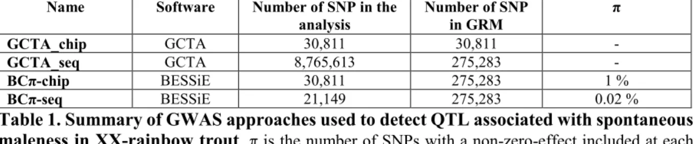
Name Software Number of SNP in the
analysis Number of SNP in GRM π
GCTA_chip GCTA 30,811 30,811 -
GCTA_seq GCTA 8,765,613 275,283 -
BCπ-chip BESSiE 30,811 275,283 1 %
BCπ-seq BESSiE 21,149 275,283 0.02 %
Table 1. Summary of GWAS approaches used to detect QTL associated with spontaneous maleness in XX-rainbow trout. π is the number of SNPs with a non-zero-effect included at each cycle k of the MCMC algorithm. GRM: Genomic Relationship Matrix
Estimation of genetic parameters
Variance components and heritability were estimated using the average information of restricted maximum likelihood analysis (AI-REML) implemented in GCTA software25 with the
same model as equation (1). The two GRM build with 31K and 257K SNPs for GWAS were used separately to estimate genetic parameters at the genome and the sequence level.
11 The values obtained with the 31K SNPs GRM were used as prior for both BayesCπ models and genetic variance(𝜎𝐴2) was calculated as the sum of the polygenic variance (𝜎
𝑈 2, estimated by
BESSiE) and the genomic variance (𝜎𝐺2) estimated by n SNPs calculated according to (3):
𝜎𝐺2 = ∑ 2𝑝𝑖𝑞𝑖𝑎𝑖2 𝑛
𝑖=1
(3)
With pi and qi the allele frequencies for the ith SNP and ai the estimated additive effect of the ith
SNP.
Genomic heritability (h²g) was estimated as ℎ𝑔2 = 𝜎𝐴 2
(𝜎𝐴2+ 𝜎 𝐸2)
⁄ with 𝜎𝐴2 the estimated genetic
variance and σ²E the residual variance.
QTL definition
For the GCTA-chip and GCTA-seq analysis, we determined chromosome-wide suggestive and genome-wide significance thresholds using a Bonferroni correction of α = 1% (genome-wide threshold = -log10(α/n); chromosome-wide threshold = -log10(α/[n/30]) with n the number of
SNP in the analysis (30,811 or 8.7 millions). Only SNPs with -log10(P-value) over the
chromosome-wide threshold for chip and over the genome-wide threshold for GCTA-seq were considered. Approximate confidence intervals (CIs) for each QTL with a peak SNP value over the significance threshold were estimated using a drop-off limit29 of 1.5 unit of
- log10(P-value) and a maximum distance of 1 Mb for the chip and 200 kb for the
GCTA-seq between two successive SNPs with -log10(P-value) over the drop-off limit starting from the
position of the peak SNP.
In the GCTA-seq, when two successive QTLs were detected at a distance lower than 50 bp and with less than 250 kb between their peak SNPs, the CIs were cumulated in a credibility interval (See Supplementary Table S1 for detailed CIs).
12 For the Bayesian approaches, the degree of association between a SNP and the phenotype was assessed using the Bayes Factor30 (BF):
𝐵𝐹 = 𝑃𝑗 (1 − 𝑃𝑗) ⁄ 𝜋 (1 − 𝜋) ⁄ (4)
With Pj the probability of the SNP j having a zero effect and π the proportion of SNP having a
non-zero effect on the trait (in our case π = 1% for BCπ-chip and π = 0.02% for BCπ-seq). BF was transformed into logBF computed as twice the natural logarithm in order to obtain values of the same usual range as the P-value, thus facilitating the visual appraisal of QTL and the comparison between methods31. To defined QTLs with the BayesCπ approaches, we defined
two categories to classify the strength of the evidence in favour of a QTL32: evidence was
consider as strong for 8 ≤ logBF < 10 and as very strong for logBF ≥ 10. Because the Bayes Factor is not a statistic test, confidence intervals cannot be derived, but credibility intervals can be built as defined in Michenet et al.33. Credibility intervals were determined using the threshold
logBF ≥ 8 for defining a peak SNP showing evidence for a QTL in either a chip or a BCπ-seq analysis. For the BCπ-chip approach, the credibility interval included every SNP with a logBF > 3 within a 1 Mb sliding window from the peak SNP. For the BCπ-seq approach, it included every SNP with a logBF > 5 within a 200 kb sliding window from the peak SNP. The proportion of genetic variance explained by each SNP was derived from the Bayesian analyses and calculated according to (5):
𝑉𝑔𝑖 =
2𝑝𝑖𝑞𝑖𝑎𝑖2 𝜎𝐴2 (5)
With pi and qi the allele frequencies for the ith SNP, ai the estimated additive effect of the ith
SNP and 𝜎𝐴2 the total additive genetic variance (as defined earlier). To estimate the proportion
of variance explained by a QTL, the proportions of genetic variance explained by all the SNPs within the credibility interval were cumulated.
13
Candidate genes and SNP annotation
Candidate genes located within a reduced interval determined as the intersection of confidence and credibility intervals estimated using both GCTA-seq and BCπ-seq analysis were listed from the NCBI Oncorhynchus mykiss Annotation Release 100 (GCF_002163495.1).
Annotation of SNPs within those intervals was performed using the SNPEff software34 (version
4.3) with the NCBI Oncorhynchus mykiss Annotation Release 100 (GCA_002163495.1)22 as a
reference. SNPs were then filtered according to their estimated putative impact, all SNPs with a modifier putative impact were filtered out and only SNP with a low, moderate, or high putative impact were conserved.
Pedigree and dams’ genotypes
Genomic pedigree information’s were recovered using identity by descent (IBD) estimates from PLINK software24 (version 1.9) using information of the 31K SNPs. The percentage of
masculinised fish in the genotyped offspring of each dam was calculated (see Supplementary Table S2). The 50 dams used in the mating scheme were named according to the proportion of masculinised fish in their offspring with the AA-dam having the higher proportion of masculinised offspring and the BX-dam having the lower proportion of masculinised offspring (Figure 1). Among the dams with at least 10 progeny recorded, the 22 dams with extreme progeny phenotypes were selected: the 11 dams (labelled from BH to BR) that had less than 8% of masculinised fish in their offspring and the 11 dams (labelled from AA to AK) that had more than 35% of masculinised offspring. Those 22 dams with extreme masculinisation rate in the offspring sample were selected for in-depth analysis of their genotypes at the QTL regions.
Results
Phenotyping, genotyping and pedigree
In this experiment we phenotyped 20,210 XX-rainbow trout from the French trout farm « Les
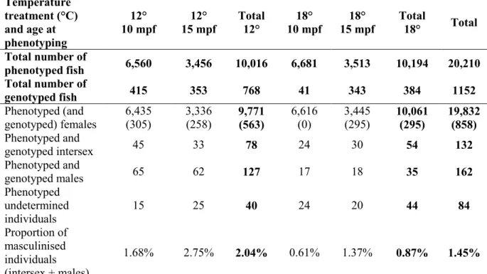
14 were partially (intersex), or completely masculinised. From the 294 masculinised individuals, 45.0% were intersex with both female and male gonadal tissues. Among these intersex individuals, 60.6% had a right gonad completely masculinised or more masculinised than the left gonad. A significant (p = 3.201e-12) higher maleness (males + intersex) was observed in the group that was reared at 12° (2.0%) than in the group reared at 18° (0.9%) (see Table 2).
Temperature treatment (°C) and age at phenotyping 12° 10 mpf 12° 15 mpf Total 12° 18° 10 mpf 18° 15 mpf Total 18° Total Total number of phenotyped fish 6,560 3,456 10,016 6,681 3,513 10,194 20,210 Total number of genotyped fish 415 353 768 41 343 384 1152 Phenotyped (and genotyped) females 6,435 (305) 3,336 (258) 9,771 (563) 6,616 (0) 3,445 (295) 10,061 (295) 19,832 (858) Phenotyped and genotyped intersex 45 33 78 24 30 54 132 Phenotyped and genotyped males 65 62 127 17 18 35 162 Phenotyped undetermined individuals 15 25 40 24 20 44 84 Proportion of masculinised individuals (intersex + males) 1.68% 2.75% 2.04% 0.61% 1.37% 0.87% 1.45%
Table 2. Phenotyping records for the XX-rainbow trout produced at “Les fils de Charles
Murgat” farm.
mpf: months post-fertilisation
From the 1,152 genotyped XX-rainbow trout, 1,139 fish genotyped for 30,811 SNPs were retained after quality controls. Pedigree was recovered for all genotyped offspring except four, the 50 dams had in average 22.7 genotyped offspring (min = 2, max = 63). The average percentage of masculinised fish in the genotyped offspring sample was 20.7%, ranging from 0% for eight females to 71.4% for the AA-dam (see Figure 1 and Supplementary Table S2). The 11 dams (labelled from dam AA to dam AK) that had the highest proportion of masculinised offspring in the genotyped sample bred 370 fish accounting for 68% of masculinised genotyped offspring. On contrary, the 11 dams (labelled from dam BH to dam BR) with a low masculinised rate among their genotyped offspring sample accounted for only
15 5% of masculinised genotyped offspring. Among those 22 dams, we detected two couples of related (IBD coefficients of 0.36) dams (AA-BK and AI-BR) with one “sister” having a highly masculinised offspring (71.4% for AA or 37.5% for AI) and the other “sister” that produce a low number of masculinised offspring (6.1% for BK or 0% for BR).
Figure 1. Total number of genotyped offspring (females, males and intersex) for each of the 50 dams (AA to BX) used in the mating scheme. The 22 dams with more than 10
genotyped offspring and extreme masculinisation rate selected for in-depth analysis of their genotypes at QTL regions are underlined.
Estimation of genetic parameters for spontaneous maleness in XX-rainbow
trout
The variance components and heritability of the sex phenotype estimated under different genomic models using either the 30,811 SNPs on the chip or the 8,784,147 SNPs on WGS are presented in Table 3. The estimated heritability of maleness was high, ranging from 0.48 with the GCTA-chip analysis to 0.62 with the GCTA-seq analysis. The estimated genetic variance (σ²A) was consistent across all models, with the lower value obtained for GCTA-chip (0.21),
intermediate values obtained with BayesCπ models (0.24 and 0.25 for BCπ-chip and BCπ-seq, respectively) and the highest genetic variance estimate (0.26) was obtained with the GCTA-seq analysis. With the increasing number of SNPs (from 31K to WGS) in the model or with the addition of a polygenic effect under a Bayesian approach, the estimate of genetic variance was increased, showing that the 31K SNPs genotyped were insufficient to capture all the genetic variation. Therefore, the real heritability of maleness is expected to be about 0.6 in rainbow trout. Analysis h²G± SE σ²P ± SE σ²E ± SE σ²A ± SE σ²U ± SE σ²G ± SE GCTA-chip 0.48 ± 0.04 0.43 ± 0.02 0.22 ± 0.01 0.21 ± 0.03 - - BCπ-chip* 0.56 ± 0.05 0.43 ± 0.02 0.19 ± 0.02 0.24 ± 0.03 0.10 ± 0.03 0.14 ± 0.03 GCTA-seq 0.62 ± 0.06 0.42 ± 0.02 0.16 ± 0.02 0.26 ± 0.03 - - BCπ-seq* 0.59 ± 0.05 0.44 ± 0.02 0.17 ± 0.02 0.25 ± 0.03 0.21 ± 0.03 0.04 ± 0.01 Table 3. Genetic and genomic parameters estimates for spontaneous maleness under the different statistical models. h²G: genomic heritability, calculated as σ²A / (σ²A + σ²E). σ²A: Total genetic variance, σ²U: polygenic variance, σ²G: genetic variance explained by SNPs, σ²E: residual
16
variance, σ²P: phenotypic variance (= σ²A + σ²E). *value of one string among the two or four used for GWAS, the string with the closest final π to the 1% or 0.02% was chosen.
Based on the BCπ-chip model, we estimated that the 31K SNPs spanning all the genome accounted for only 58% of the total genetic variance of sex (Table 3). Using the BCπ-seq model we estimated that the sequence segment spanning the 4 Mb located between 62 and 66 Mb on Omy1 accounted for 16% of the total genetic variance of sex (Table 3).
Genome Wide Association Studies of maleness in XX-female rainbow trout
GCTA-chip and BCπ-chip approaches at the 31K genotyping level
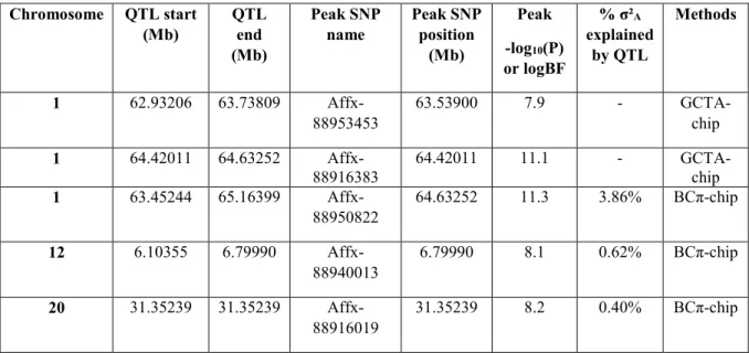
Based on the 31K SNPs, we detected four QTLs associated with maleness on three different chromosomes (Omy1, 12 and 20) with the GCTA and the BayesCπ analyses (see Table 4). With the GCTA-chip approach, we detected two QTLs on Omy1, with the first QTL being suggestive only, at 1% at the chromosome-wide level, and explaining less than 0.2% of the total genetic variance. The second QTL was significant, at 1% at the genome-wide level, under GCTA-chip analysis (-log10 (P-value) = 11.1) and had a very strong evidence under a BCπ-chip analysis
(logBF = 11.3) (Table 4). Even if the two peak SNPs of this QTL differed across the two GWAS approaches with the GCTA peak SNP being located 212 kb before the BCπ peak SNP, they were in close vicinity with only three markers in-between the two peak SNPs. This second QTL explained 3.9% of the total genetic variance. We did not distinguish the two QTLs with the BCπ-chip approach, as the credibility interval estimated with BCπ-chip was 1.7 Mb and contained the two peak SNPs detected with GCTA-chip.
The two other QTLs located on Omy12 and Omy20 were detected using the BCπ-chip approach only (Table 4). The QTL located on Omy12 explained 0.6% of the total genetic variance. The QTL on Omy20, defined by a single SNP located at 31.352 Mb, explained 0.4% of the total genetic variance. This last QTL was suggestive at 5% at the chromosome-wide level under GCTA-chip analysis (-log10(P-value) = 4.2).
17 Chromosome QTL start (Mb) QTL end (Mb) Peak SNP name Peak SNP position (Mb) Peak -log10(P) or logBF % σ²A explained by QTL Methods 1 62.93206 63.73809 Affx-88953453 63.53900 7.9 - GCTA-chip 1 64.42011 64.63252 Affx-88916383 64.42011 11.1 - GCTA-chip 1 63.45244 65.16399 Affx-88950822 64.63252 11.3 3.86% BCπ-chip 12 6.10355 6.79990 Affx-88940013 6.79990 8.1 0.62% BCπ-chip 20 31.35239 31.35239 Affx-88916019 31.35239 8.2 0.40% BCπ-chip Table 4. Summary of QTLs associated with spontaneous maleness in XX-rainbow trout: characteristics for QTLs detected with GCTA-chip and BCπ-chip methods. The QTL start and end positions correspond to the confidence and credibility intervals for GCTA-chip and BCπ-chip, respectively. For BCπ-chip, the logBF is calculated as twice the natural logarithm of Bayes Factor. The % of genetic variance, σ²A, explained by the QTL was calculated as the sum of the variance by BCπ-chip
model of all SNP in the QTL credibility interval divided by the corresponding σ²A. GCTA-seq and BCπ-seq approaches at the whole genome sequence level
Using the WGS data and GCTA-seq approach, we only detected significant QTLs on Omy1, in a delimited region in-between 62 and 66 Mb. In total six peak SNPs corresponding to six putative QTLs (see Supplementary Table S1 and Supplementary Figure S2) were detected. Therefore, the BCπ-seq approach was performed considering only the 21K SNP spanning this 4 Mb-window on Omy1 in addition to a genome-wide polygenic component. Using this approach we detected only two QTLs (see Table 5 and Supplementary Figure S3). The first putative QTL detected by the GCTA-seq analysis was not detected using the BCπ-seq approach. Therefore, it will not be discussed any further as it is likely that the association is only due to linkage disequilibrium with the SNPs included in the second QTL region. The second putative QTL detected between 63.229 and 63.774 Mb with the GCTA-seq approach was also detected with the BCπ-seq approach in a reduced credibility interval (between 63.459 and 63.556 Mb, see Table 5); it was hereafter considered as the first true QTL on Omy1.
18 The four remaining putative QTLs from the GCTA-seq analysis were very close to each other, with less than 250 kb between two successive peak SNPs, and the limits of their confidence intervals (CIs) approximated by a drop-off approach were all distant from less than 3 kb. Therefore these four CIs were fused into a single credibility interval of 342 kb. This second QTL was also detected with the BCπ-seq analysis (Table 5). While the peak SNP of the first QTL was the same under the two BCπ-seq analyses, this was not the case for this second QTL. However, the two peak SNPs were only separated by 3.2 kb and the credibility intervals were strongly overlapping (Table 5).
Based on the average of the two BCπ-seq analyses, among the 16% of genetic variance explained by all the 21K SNPs included in the BCπ-seq model, the first QTL explained about 0.5% and the second QTL explained about 14% of the genetic variance.
Chromosome QTL start (Mb) QTL end (Mb) QTL size (kb) Peak SNP name Peak SNP position (Mb) Peak SNP -log10(P) or logBF % σ²A explained by QTL Methods 1 63.229379 63.774478 545.1 Omy1-63493395 63.493395 10.61 - GCTA-seq 1 64.360291 64.707100 341.6 Omy1-64597800 64.597800 13.74 - GCTA-seq 1 63.459553 63.555809 96.27 Omy1-63520900 63.542090 12.97 0.56% BCπ-seq1 1 64.266321 64.649580 383.26 Omy1-64607018 64.607018 14.67 13.55% BCπ-seq1 1 63.459545 63.727071 267.53 Omy1-63520900 63.542090 11.55 0.51% BCπ-seq2 1 64.087947 64.632497 544.55 Omy1-64610233 64.610233 17.32 14.56% BCπ-seq2
Table 5. Summary characteristics for the two QTLs associated with maleness in XX-rainbow trout detected on the whole genome sequence using GCTA-seq and BCπ-seq methods. For GCTA-seq, the start and stop position of the first QTL correspond to a CI estimated with a drop-off approach and the start and stop positions of the second QTL correspond to the credibility interval estimated as the union of confidence intervals of four QTLs. The BCπ-seq1 and BCπ-seq2 correspond to the same analysis run with two different seeds for MCMC initialization (random number generator). Significance of peak SNP are calculated as the –log10(p-value) for GCTA-seq, and as logBF estimated as twice the natural logarithm of Bayes Factor for BCπ-seq. % σ²A: proportion of total genetic variance explained by the credibility interval of the QTL calculated using BCπ-seq approaches.
At the end of the second QTL we found a haplotype block of 15 consecutive SNPs (spanning 745 kb from 64.632011 to 64.632756 Mb) that have a significant effect on masculinisation (all the 15 SNPs have -log10(P-value) between 12.2 and 13.6 and among them five SNPs with logBF
19 > 9). For this 15 SNP-haplotype, masculinised fish were overrepresented among the homozygous genotypes for the alternative allele (different from the reference genome sequence). Interestingly, for the same block of 15 SNPs, eight of the 11 dams with almost no masculinised offspring carried two copies of the reference genome haplotype (the three remaining dams being heterozygous at these 15 SNPs). Among the 11 dams with a high rate of masculinised offspring, only three were homozygous for the reference haplotype, six were heterozygous and the last two (labelled AA and AJ in Figure 1) were homozygous for the alternative haplotype. In the offspring, the homozygous genotype for the alternative haplotype was overrepresented in masculinised fish (51.5% of masculinised fish) and underrepresented in females (8.7% of females). On the contrary, the reference haplotype was observed either at the heterozygous or homozygous state for respectively 50.6% and 40.2% of the female progeny.
Positional candidate genes and SNP annotation
In total five genes were positioned within the first QTL region spanning from 63.459 to 63.556 Mb (see Supplementary Table S3). The peak SNP from GCTA-seq (at 63.493 Mb) was located within the pygb gene (glycogen phosphorylase, brain form, from 63.487 to 63.508 Mb), and the peak SNP from both BCπ-seq runs (6.542 Mb) was located within the ninl gene (ninein-like protein, from 63.542 to 63.594 Mb). Among the 669 annotated SNPs spanning the QTL region, only 23 SNPs were indicated with either a low (16 SNPs) or a moderate (7 SNPs) potential effect on gene expressions when annotated with the SNPEff software (See Figure 2 and Supplementary Table S4). The only SNP that was both significant (-log10(P-value) = 9.6) and
annotated with a potential moderate effect was located at 63 543 061 bp within the ninl gene and annotated has a missense variant (Figure 2). This SNP was very close to the peak SNP detected by the two BCπ-seq analyses (Table 5).
Figure 2. Annotated SNPs located within the first QTL region from 63.549 to 63.556 Mb on the chromosome 1. The significance of SNP (dots) effect is given by the –log10(p-value) estimated with the GCTA-seq approach. The dark blue is the 1% at the genome wide level threshold. Putative impact of SNP on genes was estimated by SNPEff, only SNP with MODERATE or LOW effects on
20
genes are represented. Genes located within this QTL are represented by rectangle: banf1 (barrier-to-autointegration factor-like), pygb (glycogen phosphorylase, brain form), abhd12 (alpha/beta-Hydrolase domain containing 12), gins1 (DNA replication complex GINS protein PSF1), ninl (ninein-like protein).
Within the second QTL region spanning from 64.360 to 64.633 Mb, 14 genes were annotated. All the 3 peak SNPs (table 5) detected by the different WGS analyses were located in the intergenic region between the hells gene (helicase, lymphoid specific) and an uncharacterized protein (LOC110527930, see Supplementary Table S3). In total, 1,498 SNPs were annotated in the QTL region, and only 44 SNPs had either a moderate (15 SNPs) or low (29 SNPs) potential effect on gene expression (Figure 3 and Supplementary table E). Among those 44 SNPs, 12 SNPs with a potential effect on 3 genes i.e., cyp17a1 (Cytochrome P450 Family 17 Subfamily A Member 1), hells, and LOC110527930 were significant (-log10(P-value) >10) based on
GCTA-seq analysis (Figure 3). One significant SNP (-log10(P-value) = 10.2) was annotated as
a missense variant within the cyp17a1 gene (Figure 3). Two significant SNPs (-log10(P-value)
= 12.8 and 11.7) were annotated for a low potential effect on the hells gene as they corresponded respectively to a synonymous mutation and a variant within a splice region or an intron of the gene (see Supplementary Table S5). Finally, nine SNPs from the haplotype block of 15 SNPs previously identified, were annotated with either low or moderate potential effects on the LOC110527930 uncharacterized protein (see Supplementary Table S5). All the seven SNPs annotated for moderate effects were missense variants. Among them, two SNPs, located at 64 632 546 bp and at 64 632 583 bp (Figure 3), seemed to be good candidates for the causative mutation as they were both significant in the GCTA-seq and one BCπ-seq analysis (-log10
(P-value) = 13.6 and logBF > 11).
Figure 3. Annotated SNPs located within the second QTL region, from 64.360 to 64.633 Mb on the chromosome 1. The significance of SNPs (dots) is given by the –log10(p-value) estimated with the GCTA-seq approach. The dark blue is the 1% at the genome wide level threshold. Putative impact of SNP on genes was estimated by SNPEff. Only SNP with MODERATE or LOW effects on genes are represented. Genes located within this QTL are represented by rectangle: slc2a15a (solute carrier family 2, facilitated glucose transporter member 9-like), fgf8 (fibroblast growth factor 8), fbxw4 (F-box/WD repeat-containing protein 4), wbp1l (WW domain binding protein 1-like), cyp17a1 (Cytochrome P450 Family 17 Subfamily A Member 1), borcs7 (BLOC-1-reltaed complex subunit 7),
21
protein 6), zgc:175214 (RING finger protein 122-like), calhm2 (calcium homeostasis modulator protein 2), hells (lymphocyte-specific helicase-like), LOC110527930 (uncharacterized protein).
Discussion
To the best of our knowledge, this study is the first one to study spontaneous masculinisation in XX rainbow trout through a GWAS. The analysis was carried out in a rainbow trout commercial line reared either under standard temperatures (12-14.5°C) or after a high temperature treatment during early stages.
The overall masculinisation rate was 1.45%, which is in range of what is reported by several French farmers (unpublished data). Unexpectedly, the masculinisation rate was significantly higher for the group reared at the 12°C water temperature than for the group exposed to the high temperature treatment at 18°C. This result is in contradiction with the observation from Valdivia et al.15 (2014) who observed a masculinizing effect of early hot temperature treatment
(18°C vs 12°C). However, in their experiment, the temperature treatment was applied a little bit earlier (at 32 dpf, instead of 35 dpf), so the temperature we applied might have not completely overlap the critical thermosensitive period of sex differenciation35,36 inducing a
repression instead of an induction of masculinisation. This hypothesis should deserve further work to be confirmed. Different genetic backgrounds could also contribute to the observed differences in response to thermal treatment. In Validivia et al.15 (2014), the tested families
belonged to the INRA XX-mal lineage, an experimental line different from the commercial population used in this study. The hypothesis is further supported by the fact that distinct maleness QTLs were detected in INRA XX-mal families13 and in this study (see below),
suggesting that masculinizing factors may differ according to populations, resulting in different susceptibility to temperature. Indeed, different sex ratios have been reported in rainbow trout populations with various genetic backgrounds in response to temperature treatments14,37. In
other fish species such as Atlantic silverside38 or Nile tilapia39, sex differentiation is also known
22 The observed level of masculinisation was variable among masculinised fish with about 40 and 61% of intersex fish in the 12°C and 18°C groups, respectively. Within those intersex individuals, whatever the rearing temperature of fry, the right gonad was very often more masculinised than the left gonad. This particularity was first described by Quillet et al. (2004)40
and confirmed by Valdivia et al. (2013, 2014)12,15, in families originating from the INRA
XX-mal carrying line. Under norXX-mal rearing condition, the left-right asymmetry (LR) is almost
undetectable as intersex fish remain rare and poorly described. However, the observation of such an asymmetry in another rainbow trout population suggests that this a general feature in rainbow trout and that gonads in this species develop in an asymmetrical LR manner, as it has been reported in mammals, birds, amphibians and reptiles41 and in some fish42–44.
In this study, we reported high genomic heritability estimates for spontaneous maleness (from 0.48 up to 0.62) with the QTLs detected explaining only a small proportion (up to 14%) of the estimated genetic variance. Using the BCπ-chip model, we estimated that 58% of the genetic variance was explained by the pan-genomic 31K SNPs. The remaining 42% of genetic variance was probably not captured by the SNPs due to their heterogeneous density distribution across the genome and also due the inaccurate estimates (regressed towards 0) of their effects with only 1,139 phenotyped and genotyped individuals.
Concerning the identification of the genetic determinants of the maleness, we detected four QTLs on three different chromosomes, two QTLs being on Omy1, one on Omy12 and the last one on Omy20. Both QTLs on Omy12 and Omy20 were only detected in the 31K SNPs analyses and were not confirmed on WGS analyses. The QTL on Omy20 might be the result of a spurious association as it was defined by a single SNP in both BCπ-chip and GCTA-chip analysis. It is interesting to note that in their study in gynogenetic families from INRA XX-mal line, Guyomard et al.13 (2014) detected four QTLs associated with spontaneous maleness on
23 too. However, it had a wide CI, covering the entire chromosome, so it is not possible to say if the QTL we detected in the present study on Omy20 is the same and is shared between the two genetic backgrounds. As we did not detect QTL on the three other chromosomes they reported, maleness in rainbow trout with different genetic backgrounds is likely to be controlled by a variety of underlying genetic mechanisms.
The two main QTLs associated with masculinisation in our population were both detected on Omy1, which has never been reported as associated with neither sex determinism nor maleness in rainbow trout. Using WGS information, we were able to reduce the CI of the first QTL from 806 kb (GCTA-chip, Table 4) to 545 kb based on GCTA-seq analysis and even 96 kb for the credibility interval estimated with one of the BCπ-seq runs (Table 5). While highly significant, this QTL explained only 0.5% of the total genetic variance. This low proportion of variance explained may be the result of a strong linkage disequilibrium of those SNPs with some SNPs of the second QTL, which was mapped at a close distance (< 1.2 Mb between the peak SNPs of these two QTLs), making this first QTL an artefact. Within this first QTL region, no gene seems to have a functional role in gonad development; however, this QTL may contain regulating factors involved in the control of genes contained in the second QTL.
For the second QTL, the credibility interval ranged from 268 kb to 545 kb depending on the different WGS analyses (Table 5 and Supplementary Table S1). Based on the BCπ-seq analysis, we estimated that this second QTL explain about 14% of the total genetic variance while it explained less than 4% of the total genetic variance under the BCπ-chip analysis. It is difficult to know whether this proportion of variance was either overestimated under the BCπ-seq model or underestimated under the BCπ-chip model because we ignored the covariance between close SNPs estimates when deriving this proportion. Nevertheless, this QTL is explaining a sufficient part of the genetic variance to deserve specific attention in breeding programs.
24 Within this main QTL region, three genes may be potential candidates for explaining the spontaneous masculinisation. First, the fgf8a gene might be involved in the left-right (LR) asymmetrical gonad development observed in the intersex fish. This fgf8 gene is part of the fibroblast growth factor family which plays a major role in vertebrate development and has been reported to be fundamental for proper LR asymmetric development of multiples organs (brain, heart and gut) in zebrafish45. The second and biologically more convincing candidate
gene is cyp17a1 as it is a major enzyme of the steroidogenic pathway and is involved in the synthesis of biologically active gonadal androgens and oestrogens. Indeed, cyp17a1 has been identified as potentially involved in spontaneous maleness in common carp (Cyprinus carpio)46
and was recently characterized as being involved in the gonad differentiation in zebrafish with complete masculinisation phenotype in cyp17a1 deficient zebrafish47. However, in our analysis,
the only SNP with a putative missense effect for this gene was significant in the GCTA-seq analysis only (-log10(p-value) = 10.2) and had very low logBF values in both BCπ-seq approach
(0 or 2.4). However, even if the cyp17a1 gene was not within the most significant region of the QTL (in-between the hells gene and LOC110527930) in terms of significance/evidence tests, we could not exclude its implication potentially through long distance regulation of its expression. Based on the GWAS as well as the SNP annotation, the uncharacterized LOC110527930 protein was the most relevant candidate found in our analysis with a haplotype block of 15 consecutive SNPs (from Omy1-64632011 to Omy1-64632756) that were all significant (-log10(P-value) > 12) and presented alternative genotypes for 4 dams with opposite
proportions of masculinised progeny (2 dams with highly masculinised genotyped offspring and 2 dams with low masculinised genotyped offspring). In addition, seven of those SNPs were annotated with a putative missense effect on the LOC110527930 protein. However, there is no published evidence that this uncharacterized protein could play a role in gonadal sex
25 differentiation and more work is still needed to characterise this protein and its potential effect on gonadal differentiation.
The high heritability (up to 0.62) of spontaneous maleness estimated in this study opens up opportunities to manage maleness in all-female trout populations. In particular, in case the two highly significant QTLs detected on Omy1 in the present population were confirmed to play a role in spontaneous maleness in numerous other rainbow trout populations with diverse genetic origins, the identified SNPs could then be used in a cost-efficient genotyping test to identify female broodstock with a higher propensity to transmit male or intersex phenotype in their progeny. Breeders willing to limit the occurrence of undesirable masculinised individuals in their commercial all-female stocks, could target those SNPs to discard broodstock that could sire a masculinised progeny. We tested various combinations of SNPs from the two QTLs detected on Omy1 in order to maximise the efficiency of detection of the masculinised fish while keeping low the number of false positives (i.e. females) to develop a test with good specificity in our studied population. Before applying the same test in other populations, the effect of those SNPs should be confirmed in a large set of populations with diverse genetic backgrounds. Our preliminary results regarding maleness QTLs in either the XX-mal families from the INRA experimental population and the French commercial population used in this study suggest that this might not be the case. Within the main QTL (from 64.360 to 64.707 Mb), all significant SNPs would give similar results, any SNP homozygous for the alternative allele would allow the detection of 44.7 to 51.5% of masculinised fish in our sample, whereas only 6.8 to 13.7% of the homozygous fish for the alternative allele would be females. In particular, using the alternative allele of any SNP from the haplotype block of 15 SNPs described previously (between 64,632,011 and 64,632,756 bp) would allow detecting 51.5% of masculinised fish in our sample. Among those 15 SNPs, the SNP Affx-88950822 is present on the commercial 57K chip and could be of immediate use, provided its effect is found in other
26 trout populations. Every combination of two or more SNPs within this main QTL would results in a smaller proportion of false positive (less females discarded) but also in a slightly smaller proportion of males identified. Still in our samples, pairing this Affx-88950822 SNP (or any other SNP from the associated 15-SNP haploblock) with SNPs from the first QTL on Omy1 (from 63,459 to 63,556 Mb) would slightly increase the test sensitivity (identifying more masculinised fish) without eliminating too many true females.
From a breeder perspective, additional research is needed to improve knowledge about genetic basis and environmental factors determining spontaneous maleness in all-female stocks before any application in the industry. In addition to the confirmation of the existence of the same QTLs in various rainbow trout populations, the expected genetic and phenotypic responses under different thermal regimes and either pedigree-based or marker-assisted selection should be quantified to assess the efficiency of the strategy to limit the rate of spontaneous males in the production of all-female stocks. Further investigation is also needed with regard to the production of sex-reversed male breeders based on the use of spontaneous sexual inversion to prevent the use of hormones. Indeed, the high heritability of maleness suggests that the use of spontaneously masculinised individuals as progenitors of all-female populations would increase the frequency of undesirable masculinized progeny. Combining masculinising genetic factors together with an environmental (temperature) control of gonad masculinization according to the destination of the fish (broodstock vs all-female production stock) and/or the rearing environment might offer a solution to manage the trade-off. However, because of the overall low masculinization rates recorded in this study, we were not able to detect any potential interaction between rearing temperature and genotype, and we have no suspicion of the existence of such an interaction, as a GWAS with GCTA-chip, carried out with individuals from the 12°C group only, detected the same QTLs as for the overall population (results not shown). In the current state of knowledge on the effect of temperature on sexual differentiation,
27 it is too early to propose an efficient way of controlling the rearing conditions to either enhance or limit spontaneous maleness in rainbow trout. Although the prospect of using hormone-free neomales is very attractive, a potential important drawback may be to come back to the flesh quality and animal welfare issues (flesh loss of lipids, color and firmness due to precocious maturation; mortality due to Sparolegnia fungus) initially encountered in commercial stocks with XY-males.
In conclusion, in this study we detected minor genetic factors involved in maleness in rainbow trout in the absence of the master gene sdY. Two QTLs detected on Omy1 explained up to 15% of the total genetic variance of maleness in the population used in this study and we identified three candidate genes that might be involved in the masculinisation of XX-rainbow trout. Among those three genes, one uncharacterised protein (LOC110527930) was the most relevant candidate and more work would be need to characterise the potential effect of this protein on gonadal differentiation.
References
1. Devlin, R. H. & Nagahama, Y. Sex determination and sex differentiation in fish: an overview of genetic, physiological, and environmental influences. Aquaculture 208, 191– 364 (2002).
2. Martínez, P. et al. Genetic architecture of sex determination in fish: applications to sex ratio control in aquaculture. Front. Genet. 5, (2014).
3. Mank, J. E. & Avise, J. C. Evolutionary diversity and turn-over of sex determination in teleost fishes. Sex. Dev. Genet. Mol. Biol. Evol. Endocrinol. Embryol. Pathol. Sex Determ.
Differ. 3, 60–67 (2009).
4. Johnstone, R., Simpson, T. H., Youngson, A. F. & Whitehead, C. Sex reversal in
salmonid culture: Part II. The progeny of sex-reversed rainbow trout. Aquaculture 18, 13– 19 (1979).
28 5. Chevassus, B., Devaux, A., Chourrout, D. & Jalabert, B. Production of YY rainbow trout
males by self-fertilization of induced hermaphrodites. J. Hered. 79, 89–92 (1988).
6. Chourrout, D. & Quillet, E. Induced gynogenesis in the rainbow trout: Sex and survival of progenies production of all-triploid populations. Theor. Appl. Genet. 63, 201–205 (1982). 7. Yano, A. et al. An Immune-Related Gene Evolved into the Master Sex-Determining Gene
in Rainbow Trout, Oncorhynchus mykiss. Curr. Biol. 22, 1423–1428 (2012).
8. Yano, A. et al. The sexually dimorphic on the Y-chromosome gene (sdY) is a conserved male-specific Y-chromosome sequence in many salmonids. Evol. Appl. 6, 486–496 (2012).
9. Bertho, S. et al. Foxl2 and Its Relatives Are Evolutionary Conserved Players in Gonadal Sex Differentiation. Sex. Dev. Genet. Mol. Biol. Evol. Endocrinol. Embryol. Pathol. Sex
Determ. Differ. 10, 111–129 (2016).
10. Bertho, S. et al. The unusual rainbow trout sex determination gene hijacked the canonical vertebrate gonadal differentiation pathway. Proc. Natl. Acad. Sci. U. S. A. 115, 12781– 12786 (2018).
11. Quillet, E., Aubard, G. & Quéau, I. Mutation in a sex-determining gene in rainbow trout: detection and genetic analysis. J. Hered. 93, 91–99 (2002).
12. Valdivia, K. et al. Sex Differentiation in an All-Female (XX) Rainbow Trout Population with a Genetically Governed Masculinization Phenotype. Sex. Dev. 7, 196–206 (2013). 13. Guyomard, R. et al. RAD-seq mappingof spontaneous masculinization in XX doubled
haploid rainbow trout lines. in (2014).
14. Magerhans, A., Müller-Belecke, A. & Hörstgen-Schwark, G. Effect of rearing temperatures post hatching on sex ratios of rainbow trout (Oncorhynchus mykiss) populations. Aquaculture 294, 25–29 (2009).
29 15. Valdivia, K. et al. High Temperature Increases the Masculinization Rate of the
All-Female (XX) Rainbow Trout “Mal” Population. PLOS ONE 9, e113355 (2014). 16. Ospina-Álvarez, N. & Piferrer, F. Temperature-Dependent Sex Determination in Fish
Revisited: Prevalence, a Single Sex Ratio Response Pattern, and Possible Effects of Climate Change. PLOS ONE 3, e2837 (2008).
17. Baroiller, J. F., D’Cotta, H. & Saillant, E. Environmental effects on fish sex determination and differentiation. Sex. Dev. Genet. Mol. Biol. Evol. Endocrinol. Embryol. Pathol. Sex
Determ. Differ. 3, 118–135 (2009).
18. Jalabert, B., Billard, R., Chevassus, B., Escaffre, A. & Carpentier, M. Preliminary experiments on sex control in trout: production of sterile fishes ans dimultaneous self-fertilizable hermaphrodites. Ann. Biol. Anim. Biochim. Biophys. 15, 19–28 (1975). 19. Palti, Y. et al. The development and characterization of a 57K single nucleotide
polymorphism array for rainbow trout. Mol. Ecol. Resour. 15, 662–672 (2015). 20. D’Ambrosio, J. et al. Genome-wide estimates of genetic diversity, inbreeding and
effective size of experimental and commercial rainbow trout lines undergoing selective breeding. Genet. Sel. Evol. 51, 26 (2019).
21. Sargolzaei, M., Chesnais, J. P. & Schenkel, F. S. A new approach for efficient genotype imputation using information from relatives. BMC Genomics 15, (2014).
22. Gao, G. A New and Improved Rainbow Trout (Oncorhynchus mykiss) Reference Genome Assembly. in vol. 1 40 (2016).
23. Danecek, P. et al. The variant call format and VCFtools. Bioinformatics 27, 2156–2158 (2011).
24. Chang, C. C. et al. Second-generation PLINK: rising to the challenge of larger and richer datasets. GigaScience 4, 7 (2015).
30 25. Yang, J., Lee, S. H., Goddard, M. E. & Visscher, P. M. GCTA: A Tool for Genome-wide
Complex Trait Analysis. Am. J. Hum. Genet. 88, 76–82 (2011).
26. Yang, J. et al. Common SNPs explain a large proportion of the heritability for human height. Nat. Genet. 42, 565–569 (2010).
27. Habier, D., Fernando, R. L., Kizilkaya, K. & Garrick, D. J. Extension of the bayesian alphabet for genomic selection. BMC Bioinformatics 12, 186 (2011).
28. Boerner, V. & Tier, B. BESSiE: a software for linear model BLUP and Bayesian MCMC analysis of large-scale genomic data. Genet. Sel. Evol. GSE 48, 63 (2016).
29. Li, H. A quick method to calculate QTL confidence interval. J. Genet. 90, 355–360 (2011).
30. Schurink, A., Janss, L. L. & Heuven, H. C. Bayesian Variable Selection to identify QTL affecting a simulated quantitative trait. BMC Proc. 6, S8 (2012).
31. Kass, R. E. & Raftery, A. E. Bayes Factors. J. Am. Stat. Assoc. 90, 773–795 (1995). 32. Vidal, O. et al. Identification of carcass and meat quality quantitative trait loci in a
Landrace pig population selected for growth and leanness. J. Anim. Sci. 83, 293–300 (2005).
33. Michenet, A., Barbat, M., Saintilan, R., Venot, E. & Phocas, F. Detection of quantitative trait loci for maternal traits using high-density genotypes of Blonde d’Aquitaine beef cattle. BMC Genet. 17, 88 (2016).
34. Cingolani, P. et al. A program for annotating and predicting the effects of single nucleotide polymorphisms, SnpEff: SNPs in the genome of Drosophila melanogaster strain w 1118 ; iso-2; iso-3. Fly (Austin) 6, 80–92 (2012).
35. Azuma, T. et al. The influence of temperature on sex determination in sockeye salmon Oncorhynchus nerka. Aquaculture 234, 461–473 (2004).
31 36. Craig, J. K., Foote, C. J. & Wood, C. C. Evidence for temperature-dependent sex
determination in sockeye salmon (Oncorhynchus nerka). Can. J. Fish. Aquat. Sci. 53, 141–147 (1996).
37. Magerhans, A. & Hörstgen-Schwark, G. Selection experiments to alter the sex ratio in rainbow trout (Oncorhynchus mykiss) by means of temperature treatment. Aquaculture 306, 63–67 (2010).
38. Conover, D. O. & Kynard, B. E. Environmental sex determination: interaction of temperature and genotype in a fish. Science 213, 577–579 (1981).
39. Baroiller, J. F., D’Cotta, H., Bezault, E., Wessels, S. & Hoerstgen-Schwark, G. Tilapia sex determination: Where temperature and genetics meet. Comp. Biochem. Physiol. A.
Mol. Integr. Physiol. 153, 30–38 (2009).
40. Quillet, E., Labbe, L. & Queau, I. Asymmetry in sexual development of gonads in intersex rainbow trout. J. Fish Biol. 64, 1147–1151 (2004).
41. Yu, Z. H. Asymmetrical testicular weights in mammals, birds, reptiles and amphibia. Int.
J. Androl. 21, 53–55 (1998).
42. Takahashi, E. et al. Migration behavior of PGCs and asymmetrical gonad formation in pond smelt Hypomesus nipponensis. Int. J. Dev. Biol. 61, 397–405 (2017).
43. Hayakawa, Y. & Kobayashi, M. Histological observations of early gonadal development to form asymmetrically in the dwarf gourami Colisa lalia. Zoolog. Sci. 29, 807–814 (2012).
44. Strüssmann, C. A. & Ito, L. S. Where does gonadal sex differentiation begin? Gradient of histological sex differentiation in the gonads of pejerrey, Odontesthes bonariensis (Pisces, Atherinidae). J. Morphol. 265, 190–196 (2005).
45. Albertson, R. C. & Yelick, P. C. Roles for fgf8 signaling in left–right patterning of the visceral organs and craniofacial skeleton. Dev. Biol. 283, 310–321 (2005).