Automated cameraman

Automated Cameraman by

Yaser Mohammad Khan

B.S. Electrical Engineering and Computer Science Massachusetts Institute of Technology 2010

Submitted to the Department of Electrical Engineering and Computer Science in Partial Fulfillment of the Requirements for the Degree of

Master of Engineering in Electrical Engineering and Computer Science

MASSACHUSETTS INSTITUTE OF TECHNOLOGY at the Massachusetts Institute of Technology

AUG

June 2010

LIBRARIES

ARCHIVES

electronic copies of this thesis document in whole and in part in any medium now known or hereafter created.

Author

Department of Electrical Engineering and Computer Science May 21, 2010

Certified by

D ",hristopher J. Terman

Senior Lecturer, Department of Electrical Engineerirrg and Computer Science Thesis Supervisor

Accepted by

I Christopher J. Terman

Automated Cameraman by

Yaser Mohammad Khan

Submitted to the Department of Electrical Engineering and Computer Science on May 21, 2010 in Partial Fulfillment of the Requirements for the Degree of

Master of Engineering in Electrical Engineering and Computer Science

1 ABSTRACT

Advances in surveillance technology has yielded cameras that can detect and follow motion

robustly. We applied some of the concepts learnt from these technologies to classrooms in an

effort to come up with a system that would automate the process of capturing oneself on video

without needing to resort to specialized hardware or any particular limitation. We investigate

and implement several image differencing schemes to detect and follow motion of a simulated

lecturer, and propose possible future directions for this project.

Thesis Supervisor: Christopher J. Terman

2

6.3.1 Basic Algorithm and Parameters ... 25

6.3.2 Analysis ... 31

6.4 Codebooks ... 34

6.4.1 Basic Algorithm ... 34

6.4.2 Analysis ... 35

7 Im plem entations and results... 37

7.1 General considerations ... 37

7.1.2 Movement Zones ...-... --... 39 7.2 Thresholding ...----...---.... ---... 40 7.2.1 Implementation ... 40 7 .2 .2 R e su lts ... 4 2 7.3 Histograms... ₄₇ 7.3.1 Implementation ... 47 7.3.2 Results ...---. . ---... 48 7.4 Codebooks ... . --...----... 53 7.4.1 Implementation ... .... ---... 53 7.4.2 Results ... 54 8 Future work...54 9 Conclusion...56 10 W orks Cited ... 57 11 Appendix A ... 60 12 Appendix B ... 61 13 Appendix C ... 65 14 Appendix D ... 69

3

LIST

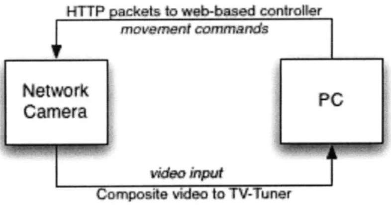
Figure 3.1: The interaction between PC and the camera ... 15

Figure 4.1: A very basic background differencing scheme. Two frames (luma components) are

subtracted and thresholded to binary (1-bit) image. A morphology kernel is then applied to

clean up noise, and a center of movement is calculated to which the camera is directed.. 21

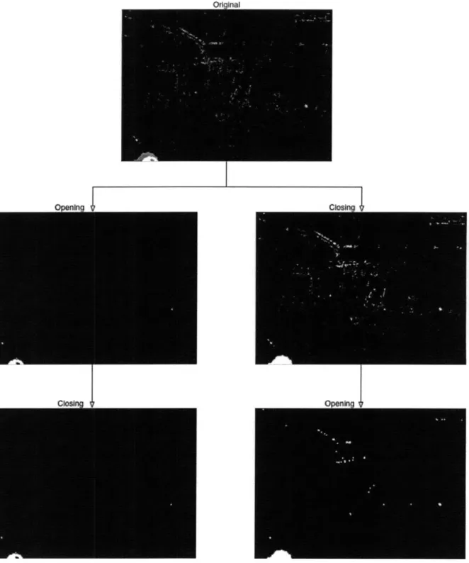
Figure 4.2: Morphological operations performed on a thresholded binary difference image. The

original has movement on the lower right corner, but everything else is noise. Opening

removes noisy foreground pixels (white), while closing removes noisy background pixels.

The order of the operations matters, as is evident from the figure. We used opening first

and then closing, because it was more important to eliminate noisy foreground pixels (that

might affect the center of movement) than noisy background pixels (which won't affect

center of m ovem ent). ... 23

Figure 4.3: A basic summed histogram scheme. A difference matrix is summed in both x-and

y-dimensions and normalized to yield significant peaks, which indicate movement. ... 26

Figure 4.4: Raw histograms for images between which no movement happens. Notice the range

of the raw data and compare it with the range in Figure 4.5. ... 27

Figure 4.5: Raw histograms for images between which movement does happen. Notice the

range of data, and compare the values of the peaks here to those of the peaks in Figure

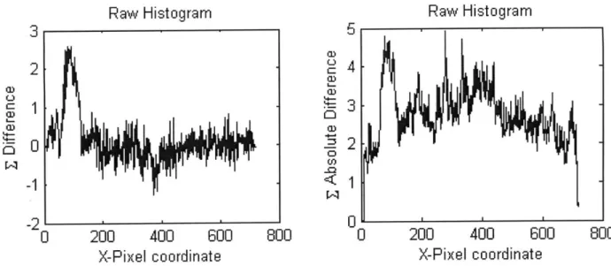
Figure 4.6: The noise tends to cancel itself out when summing differences, but adds up when

summing absolute differences (sometimes to the point of occluding the actual peak)...29

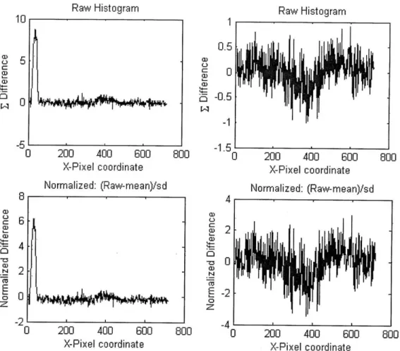
Figure 4.7: Raw and Normalized histograms of movement (left) and no movement (right). Noise

tends to keep most points within 4 standard deviations, whereas movement has points

significantly above 4 standard deviations. ... 30

Figure 4.8: An example of a false positive. There is no movement, yet a point lies above 4

standard deviations. Unfortunately these incidences happen more frequently than desired.

... _{3 0}

Figure 4.9: Sequence of histograms when the camera is moving (in the x-direction) while the

object is stationary. For the most part, the motion smoothens the histogram (particularly

the x-direction). However, there are peaks above 4 standard deviations (especially in

y-h isto g ra m s)...3 ₃

Figure 4.10: An example of how the codebook method would work. It first learns the

background by generating pixel ranges in between which most background values lie. It

also keeps track of how frequently each of the range is hit while learning the background.

Stale entries that have not been hit for a while are probably noise or foreground values

and a regular removal of stale values keeps them out of the codebook. The prediction

phase can then assess whether an incoming pixel value falls within the background range, in which case it is labeled background, otherwise it is classified as foreground. The

algorithm intermediately goes through learning and prediction phases to keep the

Figure 5.1: Contrasting-enhancing approaches, showing how an image is affected along with its

histogram. Note that in the original, most of the pixels seem to occupy a narrow range in

the middle of the spectrum, leaving the rest of the spectrum empty and wasted. PIL's

implementation takes the same histogram and just stretches it out across the spectrum, so

that pixels utilize the full width of the spectrum Linearized cumulative histogram

equalization also stretches out the pixel values across the spectrum, but tries to keep the

cumulative distribution function constant, thereby ensuring that the pixel values are more

or less evenly distributed. ... 38

Figure 5.2: An example of a video analysis frame. The top left image is the luma portion of the

actual incoming frame with movement zones drawn on top. A crosshair also appears if

movement is detected. The top right image is the reference image. The bottom left image

is the thresholded image, whereas the bottom right is the thresholded image after noise

reduction with morphology operators. Note that even though there was no movement,

the thresholded image shows up some foreground pixels (which are removed by

morphology operators). The noise free mask does not have any foreground pixels, thus no

crosshair appears in the top left corner... 42

Figure 5.3: A sequence of frames showing the system behavior over a still camera but a moving

object. Crosshairs mark movements. Note that the reference images are blurred

sometimes (because they are averages of the past 3 frames). Also note the importance of

Figure 5.4: A series of panels showing how the algorithm fails. For each panel, the actual scene

being seen by the camera is shown by the left picture, and the algorithm internals at the

very same instant are being shown by the corresponding video analysis picture on the

right. A: Subject has entered the real scene, but the algorithm doesn't see it yet. B: Subject

is about to exit the scene, and the algorithm still doesn't see anything (it is still processing

old frames). C: Subject finally enters the scene in the algorithm picture, causing the

algorithm to direct the camera to move to where it thinks it is, even though in current

time, the subject is on the opposite edge. D: The camera moves and looses the subject. E:

The algorithm still sees a person, but in actuality, the subject has been lost. F: Cache is

flushed, the algorithm and the actual camera will both see the same thing again now, but

the subject has been lost. ... 45

Figure 5.5: A sequence of pictures depicting how well the thresholding algorithm tracked once

the frame rate was reduced. A: The initial scene. B: A subject enters the scene. C: The

camera immediately moves towards the subject. D: The subject moves to the right edge of

the camera frame. E: The camera follows. F: The subject starts walking towards the left edge of the camera frame. G: The subject nearly exits the frame. H: But the camera

immediately recovers and recovers the subject. I: The subject stays in the center and

moves around, but the camera holds still and does not move. Note: The subject was

w alking at norm al speed. ... 47

Figure 5.6: Another example of a video analysis frame. The top left image is again the current

detection. The top right image is the reference image. The bottom left image is the

difference matrix summed in the y-direction (projected onto the x-axis), whereas the

bottom right image in the difference matrix summed in the x-direction (projected onto the

y-axis). ...-- .... . ---...--- 49

Figure 5.7: A series of panels showing the run of the histogram algorithm. A: No object in view,

the y-histogram is particularly noisy and above threshold, but absence of x above the

threshold ensures no movement is detected. B: An object moves into view and is reflected

in the x-histogram, but the y-histogram remains noisy. C: The x-histogram shows two

well-behaved peaks, but they're not above the threshold, so are discarded. D: Both histograms

are above the threshold now, but the y-histogram has single point peaks, thus those peaks

are disqualified. E: y-histogram is noisy again, thus no movement is detected still. F: Finally

som e m ovem ent is detected... 50

Figure 5.8: Two examples of false positives. Both occur in movement zones (near the top).

Unfortunately, this algorithm seems to emit a lot of false positives. ... 51

Figure 5.9: A sequence of images that depict how the camera reacted with the histogram

algorithm. It tracked very loosely until 00:24 at which point it completely lost the subject

4

A valuable tool in the arsenal of the modem education system is the advent and use of video cameras. With the growing proliferation of online education, as well as open courseware initiatives such as MIT Open Courseware (OCW), it has become imperative to provide some interactive mode of instruction other than simple written records or notes. While nothing beats the classroom experience, an adequate substitute is a digital video of the event, which not only enables the content to be distributed to a larger number of people, but also provides means to keep record of the event (this may be important to, say, a lecturer who may have forgotten how he explained a certain topic before, or to a student, who perhaps doesn't remember or couldn't write down what the lecturer was saying fast enough).

Recording video requires remarkably little equipment (just a video camera), but it does require two people to participate. One is the subject, who gets videotaped; the other is the cameraman, who does the videotaping. One may get away with not using a cameraman, instead fixing the camera on a tripod and staying within the camera frame being videotaped. However, this method is impractical for a number of reasons, one of which is that the lecturer doesn't know when he's not in frame (he may go slightly out of frame occasionally), and the other being the restriction of movement in the lecture hall (most lecturers like to make use of the space allotted to them). These reasons make it almost a certainty that a cameraman is present when the lecture is being recorded.

Advances in video surveillance security cameras have led to the popular use of pan-tilt-zoom (PTZ) cameras. These cameras are close-circuit television cameras with remote motor

capabilities. If these are substituted for the cameras normally used in lectures, there may be a practical way of automating the role a cameraman normally takes in the videotaping, by having these cameras move themselves instead of having a human move them.

We decided to investigate techniques that would reliably allow the automated motion of a

camera tracking a moving object, specifically a professor in a lecture hall. Because standard PTZ cameras won't do custom image processing (nor are they computationally very powerful), we

decided to use a computer to accomplish that task for us, and in the end just tell the camera where to go. We will first examine the test setup used to simulate the situation [Chapter 3],

followed by a description of the few algorithms we explored [Chapter 4], and our specific implementation of them and results [Chapter 5]. We will conclude with remarks on the future of this project and what needs to be done before the project is ready [Chapters 6 and 7].

5

SETUP

The test rig consisted of the following hardware set up:

1. Network Camera: Panasonic KX-HCM280. This was a standard Pan-Tilt-Zoom (PTZ) Camera with a built-in web-based controller interface. It also had composite video output connections.

2. TV-Tuner card: Hauppauge WinTVPVR-500. Only the composite input of the card was used.

3. Processing machine: A stock Intel Core i7 920 with 12 GB of 1066MHz DDR3 RAM running Ubuntu 9.10 ("Karmic Koala") with kernel support for TV-Tuner card. In addition the following software utilities were used:

1. ivtv-utils: This is a package available on Ubuntu. Useful for controlling the TV-Tuner

card.

2. pyffmpeg: Python module used for grabbing video frames from the card video stream.

3. numpy/scipy/matplotlib/PIL: A number of python modules for performing image

processing

The camera was connected to the web (through an Ethernet cord) as well as to the processing machine (via a composite cable to the TV-Tuner card). However one peculiarity resulted as a consequence. The web-based interface and controller only support two display modes: 320x240 and 640x480. The default output format of the composite video though was 720x480 (standard NTSC). The two incompatible resolutions posed problems later when comparing the images from the two different sources in order to determine the location of corresponding objects. In order to standardize things, a program packaged with ivtv-utils, v412-ctl was used to scale down the composite video input to the TV Tuner card from 720x480 to 640x480.

The ivtv video4linux drivers are built in to the Linux kernel from 2.6.26 onwards. As such, the set up of the TV-Tuner card is a matter of plugging it in and rebooting the machine (Ubuntu should automatically detect it). However, the control of the card is still performed through an external utility like v412-ctl, which can change inputs (by default, the input is set to Tuner, when, in our case, Composite is needed), scale resolutions (from the default 720x480 to 640x480) and perform numerous other related tasks.

Figure 5.1: The interaction between PC and the camera

Though the composite video output of the camera is enough for getting frames to perform processing on, an Ethernet connection to the PTZ is also required for accessing the camera controller and issuing move commands. So, while the composite video serves as the sensor branch, the web interface serves as the motor branch to the camera [see Figure 5.1]. The controller itself is a script hosted on the camera's web server called nphControlCamera. The various arguments to the script were reverse engineered from the camera's web interface, and it is worth it to go over them.

The way the camera moves is that you provide coordinates to it relative to the current frame (and its size), and the camera moves such that those coordinates become the center coordinates of the new camera position. If you specify coordinates that are already the center coordinates of the current frame, the camera won't move at all.

The controller requires HTTP packets in the form of POST data to determine how to move [see Appendix Afor sample code]. It takes in seven arguments:

1. Width: Only supports either 640 or 320

2. Height: Only supports either 480 or 240

4. Language: Default is 0 but other values are fine

5. Direction: Default is "Direct," but unaffected by other values

6. PermitNo: A random number string the function of which is still unknown

7. NewPosition: A tuple that contains the x and y coordinates of the center of the frame you

wish to move to. In other words, this variable takes in the x and y coordinates of a pixel in the current frame that becomes the center pixel in the new frame. NewPosition.x holds the x-coordinate, whereas NewPosition.y holds the y-coordinate.

Four of the seven variables (Title, Language, Direction and PermitNo) seem to contribute nothing to the actual movement. Alteration of their values does not seem to impact the

movement of the camera in any way. For example, PermitNo is hardcoded to a value 120481584 in our implementation of the code, but could easily be anything else (the web interface seems to change this value periodically at random).

The other three variables (Height, Width and NewPosition) are important for the movement of the camera. The new position is calculated relative to the height and width specified. For example, specifying a value of <320,240> for NewPosition while the Width and Height are specified to be 640 and 480 respectively causes the camera to not move at all (because those coordinates already specify the center of the current frame). However, having the same value for NewPosition while specifying the Width and Height to be 320 and 240 respectively causes the camera to move to the lower right (so it can center its frame on the lower right pixel specified by the coordinates).

There is one more crucial piece of information. When multiple command moves are issued, the camera controller queues them up and then executes them in order. This can be disastrous if two

command moves are issued with reference to a particular frame, but since the camera controller executes the second only after the first move has been completed, it may execute the second with reference to the wrong frame. A good example is when a camera detects movement in a corner of frame 1 (say, at [0,0]) and decides to move towards it. While moving, it passes through frame 2, where it detects another movement at [0,0], so the system issues another move command. However, because the camera is still moving, it does not execute the command, but instead queues it. The camera stops moving at frame 3, when the [0,0] coordinate of frame 1 is the center coordinate. Now it starts executing a move to [0,0] again even though it is relative to frame 3 and not frame 2 (where the movement was detected). Thus we end up in a frame that is centered at [0,0] of frame 3 instead of being centered at [0,0] of frame 2.

Other specifications of the camera are unknown. We have no information about how long it takes to move to a given coordinate. We also don't know the size of the movement queue. When provided with wrong information (for example a coordinate outside the frame), the controller simply seems to ignore it.

6

6.1

The context of the camera we envisioned was in the back of a classroom, trying to follow a professor teaching. Several observations need to be made regarding this context:

1. Because the data feed is probably in real-time, heavy duty image processing cannot be done because the camera needs to know quickly what position to move to before the object moves out of the frame.

2. A move command should be avoided from being issued every frame because we don't know how long it takes to complete a move. The movement queue feature of the camera is a problem here, because the camera will continue moving long after it should have stopped.

3. There needs to be some movement tolerance, not just for accommodating noise, but also for eliminating jitter. A very shaky camera would result otherwise, because even a slight movement would cause a move command to be issued.

4. The background is dynamic. There will be heads of students moving around in the background, and the background itself might change after the camera moves.

5. The method needs to be general enough such that it follows all professors provided they don't wear very specific clothing that exactly matches the background.

The basic class of algorithms most suited to the context above are known as background

differencing algorithms [1][2]. Background differencing is an image processing technique where change is detected between two images by finding some measure of distance between the two

(usually just subtraction). The two frames are called the reference frame and current frame. The technique is attractive because of its low computational overhead and conceptual simplicity. It is a particularly useful option when most of pixels in the two pictures are similar, and there are only slight alterations between the two. Thus, it is well suited for videos, because successive frames in videos usually have little change between them.

Subtraction of two images very similar to each other yields a lot of values close to zero, with the values only significantly diverging if the pixel values of the two images are vastly different.

Portions of the image that are relatively constant or are uninteresting are called background, whereas the interesting changes are known as foreground. Segmentation of the background and the foreground is the key concept that drives most of the algorithms in this class. In our

discussion above we assumed that the reference image contains the background, thus anything new added to the background must be in the current image (which we can locate by background subtraction). However, it is not always so easy to obtain a background and fit it in one reference frame. We will discuss a few schemes we implemented along with a motivation for why we implemented them, and then discuss the results we achieved with each.

6.2 THRESHOLDING

6.2.1 Basic Algorithm

The simplest way to segment a scene from two images into background and foreground pixels is to establish a threshold. If the difference between corresponding pixels from the two images is smaller than the threshold, then it is considered a minor difference (probably due to noise), and that pixel is labeled background, otherwise, if the difference is bigger than the threshold, then it is deemed significant, and the pixel is declared foreground. The process is known as thresholding

[see Figure 6.1]. The schema described assumes a binary value for each pixel (either it's a foreground or it's a background), but this need not be the case always. A weighting factor may be applied to assign the degree to which we are confident a certain pixel is foreground or

background (perhaps based on how close it is to the threshold). For our purposes, we will always treat it as binary.

The resulting thresholded (often binary) matrix is called the mask. It marks regions where the differences are too big as foreground, and regions where differences are small as background. The value for the threshold determines the sensitivity of foreground detection, but that can be tinkered to find good thresholds [3]. Because most of the change that happens is along the luma axis and less so along the chroma axis, color information can usually be ignored in differencing and subsequent thresholding.

As expected, thresholding isn't a perfect way of removing noise. Even though it offers a tolerance level for varying values of a background pixel between successive frames (the variation is due to noise), there will always be background pixels above that threshold. If we raise the threshold too high, we risk missing some actual foreground. So after the preliminary mask is created, we use morphological operators to clean up noise.

Once the segmentation and clean up is done, the foreground centroid can be calculated as the center of movement, which gives us a point to direct our camera to. As mentioned before, the center of movement may be calculated by using a binary mask, or it can be calculated by a weighted difference matrix.

Frame 0

Difference Thresholded

Figure 6.1: A very basic background differencing scheme. Two frames (luma components) are subtracted and thresholded to binary (1-bit) image. A morphology kernel is then applied to clean up

noise, and a center of movement is calculated to which the camera is directed.

6.2.2 Morphological operations

Mathematical morphology was developed by Matheron and Serra [4][5][6] for segmenting and extracting features with certain properties from images. In a thresholding scheme, every pixel is treated independent of surrounding pixels, which is not often the case (objects usually occupy more than one pixel). The intuition behind using morphological operations for cleaning noise is that, unlike objects, noise is usually spatially independent. Therefore, if there is one pixel that has been segmented as foreground among a number of pixels that are all background, then this pixel is probably just a false positive (that is, it's really just a background pixel, because

everything else surrounding it is also background).

There are two basic morphology operators: erosion and dilation. Both use a kernel with an anchor/pivot point. Erosion looks at all the points overlapping with the kernel and then sets the pivot point to be the minimum value of all those points. Dilation does the same except the pivot point gets assigned the maximum value of all the overlapping points. Erosion tends to reduce

foreground area (because foreground pixels are usually assigned the higher value in a binary segmentation scheme), whereas dilation increases it (consequently reducing background area). The problem with erosion is that though it is effective in removing false positives ('salt noise'), it also chips away on the true positive areas of the foreground. A combination of the two operators may be applied which approximately conserves the area of the foreground. Opening is a

morphological operation delineated by first erosion and then dilation, both by the same kernel. It preserves foreground regions that have similar shape to the kernel or can contain the kernel. It sets everything else to be the background, thus getting rid of small noisy foreground pixels [see Figure 6.2].

Closing is the dual of opening (opening performed in reverse) and is defined by performing dilation first and then erosion. It tends to preserve background regions that have the same shape as the kernel or can fit the kernel. Dilation itself can be used for filling in holes of background pixels ('pepper noise') when they are surrounded by foreground pixels, but the problem is that it tends to chip away on the boundaries of the actual background also. Performing erosion

following dilation mitigates this effect, thus getting rid of noisy background pixels without encroaching too much of the actual background territory [see Figure 6.2].

Co

Figure 6.2: Morphological operations performed on a thresholded binary difference image. The original has movement on the lower right corner, but everything else is noise. Opening removes noisy foreground pixels (white), while closing removes noisy background pixels. The order of the operations matters, as is evident from the figure. We used opening first and then closing, because it was more important to eliminate noisy foreground pixels (that might affect the center of movement) than noisy

6.2.3 Analysis

Image differencing seems to be the right way of thinking, but there are a few problems. This framework has a nice capability of being general enough that it does not depend on any

particular image in question [7]. However, it has the crucial problem of being limited to a static background (thus being unable to segregate a moving background from foreground). Earlier work also faced the same problem, with Nagel [1] quoting, "The literature about scene analysis for a sequence of scene images is much sparser than that about analyzing a single scene."

Original work done on the automated tracking of cloud motion in satellite data (for estimation of wind velocity) [8] seems too specific and difficult to generalize to other scenes. Other work [9] analyzed vehicle movements in street traffic, wherein they used the cross-correlation of a template vehicle (initially interactively selected from a particular frame), to find the location of the vehicle in the next frame. A window around the new location then becomes the new template to be used for cross-correlation in the following frame. This process iterated over a sequence of images thus follows the movement of a car. Some tolerance from noise is afforded by the dynamic update of the template at each frame, but the process as a whole can easily go wrong with the wrong choice of templates, and moreover does not address the question of dynamic or moving background. Another work [10] describes the tracking of prominent gray features of the objects, but this requires the objects to have specialized features that can be identified as

'prominent,' and also only tracks objects one at a time. Nagel [1] generalizes the framework to extract moving objects of unknown form and size, but his method also doesn't deal with moving cameras and requires image sequences where the object does not occlude the background (thus the background is extracted from image sequences where the foreground does not occupy that particular space).

Thus, in general, the major problem with this scheme seems to be its inability to model and handle a moving background (such as wind blowing through trees). A dynamic background causes problems by causing everything to be classified as foreground (and thus movement). In our context, every time the camera moves, everything in the new frame is very different from the reference frame, confusing the algorithm into thinking that everything is part of the foreground and making the camera prone to moving again.

To make a better scheme, an attempt must be made to study or at least mitigate the effects that camera movement has on background generation (by either disqualifying all frames received during movement as ineligible for forming a background, or simply not allowing any movement in the period of time immediately following a previous movement until a new reference image has been generated to compare with the new frames to make a proper decision). A method that may help us do that requires histograms to segment images.

6.3

6.3.1 Basic Algorithm and Parameters

An alternative method to thresholding (for segmentation) is to use summed histograms in x, and y dimensions. This requires the difference matrix to be summed in both the x and the y directions to obtain two histograms. These two histograms are normalized and everything above a certain threshold is defined as movement. The centroid of these points can then be designated the center of movement, and the camera instructed to move to that point [see Figure 6.3].

Frame 0

D iterence

Sur inx direcjonl Change

No rmaze Computecen toid o

r oints above certainl threshol

Figure 6.3: A basic summed histogram scheme. A difference matrix is summed in both x-and y-dimensions and normalized to yield significant peaks, which indicate movement.

The types of histograms expected (given a static background) are shown in Figure 6.4 and Figure 6.5. When no movement happens between two images [see Figure 6.4], most of the activity in the histogram is associated with noise and thus usually falls within a narrow range. There are false peaks, but usually not significant enough to pose as actual movement (this is a challenge that the normalization scheme must address). On the other hand, when actual movement occurs [see _{Figure 6.5], it shows up in the histogram as a significant peak dominating all the noise.}

Histogram in the y-direction

200 300 y pixel coordinate x pixel coordinate

Figure 6.4: Raw histograms for images between which no movement happens. Notice the range of the raw data and compare it with the range in Figure 6.5.

Because it does not matter whether an object has appeared or disappeared in the new frame, there is a temptation of summing absolute differences along a given coordinate, rather than just the differences. However, this idea is a bad one because when summing just differences, some of the noise tends to cancel itself out, but adds up when summing absolute differences [see Figure 6.6].

The spiky behavior of the histogram in the nonmoving profile shows how noisy the signal can be despite absence of movement. Preprocessing filtering is a good idea that might remove some of noise. A filter kernel is applied to each pixel and changes the value of the pixel depending on the

surrounding pixels (for example the median filter sets the value of the pixel to be the median of the surrounding pixels). A number of filters can be useful, in particular the median filter (most useful for salt-and-pepper kind of grainy noise in the image that was usually the case with our camera) and the Gaussian filter (smoothens noise in general).

Frame 0 Frame 1

Histogram in the x-direction

400 x pixel coordinate

Histogram in the y-direction

100 200 300 400 5

y pixel coordinate

Figure 6.5: Raw histograms for images between which movement does happen. Notice the range of data, and compare the values of the peaks here to those of the peaks in Figure 64.

5 -0 -5 -10 -15 -20 -25 -30 0

3 C, 2 ' ' _aD C) 3 CDC 00 20 0 0 800 20 40 0 li 0 2 -1 <1 -21 0 U 0 200 400 600 800 0 200 400 600 800

X-Pixel coordinate X-Pixel coordinate

Figure 6.6: The noise tends to cancel itself out when summing differences, but adds up when summing absolute differences (sometimes to the point of occluding the actual peak).

The normalization of the raw histograms is another important aspect that needs to be addressed.

The initial (really bad) normalization scheme was to normalize to the maximum absolute value of the histogram (making the range of the data between 1 and -1), and then specifying movement as everything above 0.8 or below -0.8. The most obvious problem with this normalization

scheme is that it will produce a movement centroid even when there isn't one (because even images with no movement will have a noise peak that will get mapped above 0.8 or below -0.8).

Another alternative means of normalization is to find the z-score for each histogram data point

(by subtracting the mean and dividing by the standard deviation). If the noise follows a normal

distribution then 99.7% of the points should fall within 3 standard deviations. Thus, if a point is above, say, 4 standard deviations, then it must be movement (with a high degree of probability)

[see Figure 6.7]. However, even this notion is prone to errors and false positives [see Figure 6.8]. Raw Histogram

Figure 6.7: Raw and to keep most points

Raw Histogram 800 1 0.5 0 -0.5 -1.5L 0 800 200 400 600 X-Pixel coordinate Normalized: (Raw-mean)/sd 0 200 400 600 X-Pixel coordinate 800 800

Normalized histograms of movement (left) and no movement (right). Noise tends within 4 standard deviations, whereas movement has points significantly above 4

standard deviations. Normalized: (Raw-mean)/sd Raw Histogram 600 0 200 400 Y-Pixel coordinate 600

Figure 6.8: An example of a false positive. There is no movement, yet a point lies above 4 standard deviations. Unfortunately these incidences happen more frequently than desired.

0 200 400 600 X-Pixel coordinate Normalized: (Raw-mean)/sd 0 200 400 600 X-Pixel coordinate 0 200 400 Y-Pixel coordinate Raw Histogram

6.3.2 Analysis

The method is limited in scope and use for many reasons. It is prone to noise and thus detects a lot of false positives, causing the camera to sometimes move without any apparent reason. However, it does seem to work slightly better than thresholding, for one particular reason: it tends not to 'see' movement when the camera is moving.

First, a similar observation to that made for thresholding can be made here: noise is spatially independent (most of the peaks occur alone). This observation can be used to mitigate the effects of noise by using a peak clustering algorithm to detect how many points a certain peak has. If a peak is just a single point, then there is a high probability that it is just noise. However, if a peak consists of multiple points, then there is a spatial correlation and it is probably significant. Thus, peaks that have below a certain number of points can be designated noise peaks (and thus not considered movement). Other peak finding algorithms [11] may also be implemented which reliably find a proper peak. A note to make here is that these algorithms introduce additional complexity in the form of more parameters to the model, whose values need to be tinkered with for an optimum to be found.

Other ways of mitigating noise factor is to average of several frames for the reference. A particular reference frame may have a noisy pixel that has an atypical value (due to noise). However, if several frames are averaged together, the effect of noise is considerably diminished (because other frames will have the proper value of that pixel), and the pixel value appears closer to its actual mean. The downside to using this method is that averaging many frames while the

camera is moving might be a bad idea because then the reference will have the mean of many different values.

The reason this method is interesting is because it allows us to study the effects of a moving camera on the image differences. This scheme (like the previous thresholding scheme) assumes a static background, and it was initially unclear what effect the movement of the camera has. It turns out that the method tends to ignore movement while the camera is in motion. While the camera is moving, everything is changing sufficiently such that the standard deviation of the data is large, thus most points fall within a few standard deviations (and don't qualify as movement). This is an improvement over our previous thresholding method because in the thresholding method, once the camera started moving, everything was always considered foreground, so the camera never stopped moving. In this method, once the camera starts moving, it is difficult to make it notice something as foreground, so tends not to move again. Once the camera stops moving, the background establishes quickly again, and the camera can move again. This phenomenon is true for most cases, but does fails sometimes [see Figure 6.91.

It is worth noting the smoothing effect camera movement has on the histograms. Generally, this fact makes the method insensitive to object movement parallel to the camera motion while the camera is in transition, and very sensitive immediately after transition. So once a move command has been issued, the camera is more likely to move again.

Thus this method, while better than thresholding (because it does not 'see' movement most times when the camera is moving), still fails often enough to warrant a more explicit modeling of a

frames 1-2 frames 2-3 6 U)4 2 -2 -4 4 2 0 ) (D -2 200 400 y-pixel coordinate frames 4-5 x-pixel coordinate 200 400 y-pixel coordinate 6 U) 4 2 a) 0 -2 -4( 6 x-pixel coordinate 0 200 400 y-pixel coordinate frames 5-6 x-pixel coordinate 4 2 0 a) S-2 -4 -6 . . 0 200 400 y-pixel coordinate x-pixel coordinate 200 400 y-pixel coordinate frames 6-7 0 200 400 600 x-pixel coordinate 0 200 400 y-pixel coordinate 0 200 400 600 x-pixel coordinate 6 4 -2 C a) 0 C-) C ,~-2 -4 0 200 400 y-pixel coordinate frames 7-8 x-pixel coordinate 10 5 0 -5 -10. 0 200 400 y-pixel coordinate

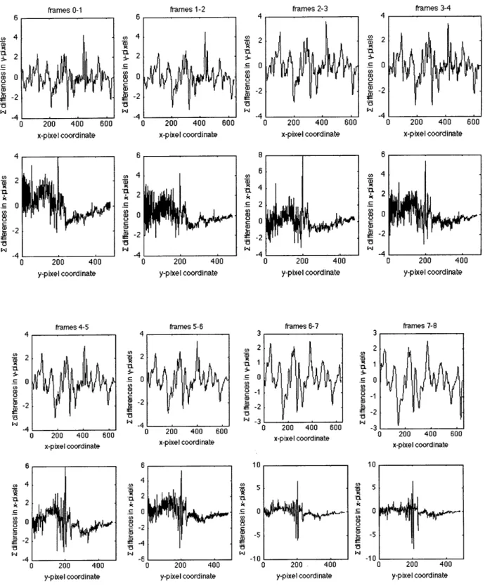
Figure 6.9: Sequence of histograms when the camera is moving (in the x-direction) while the object is stationary. For the most part, the motion smoothens the histogram (particularly the x-direction).

However, there are peaks above 4 standard deviations (especially in y-histograms)

x-pixel coordinate S2 CO L) -2 -4 6 4 .CI 3k 2 C a) 0 S-2 -4 frames 3-4 frames 0-1

6.4 CODEBOOKS

6.4.1 Basic Algorithm

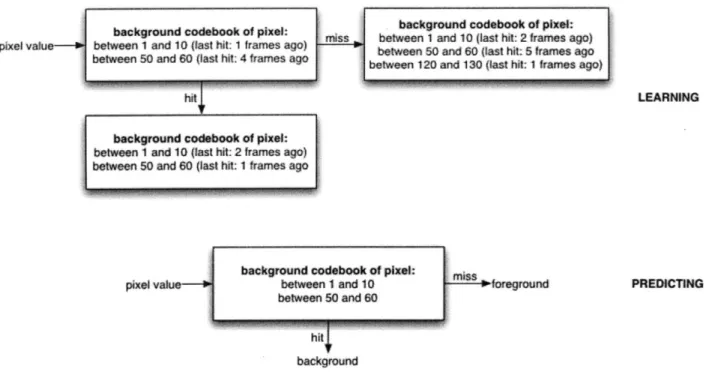
A simplistic perspective for modeling a dynamic background was provided by Kim [12][13]. They use a data structure known as 'codebooks' to hold information about the background model. Each pixel carries its own codebook, which is created during a specified training period. A codebook consists of ranges of pixel values that are found on that pixel during the specified training period. During the training period, if a particular pixel value doesn't fall under an existing entry in the codebook (i.e. a range of values), then a new entry is created for it. Otherwise the existing entry is updated to contain that pixel value. A record is kept for which entry does not get hit often, and these 'stale' entries are deleted on a periodic basis, particularly at the end of a learning period (because they're either noise or foreground). Once the learning period is over, the algorithm analyzes each pixel of the incoming frame and determines whether the new value hits one of the entries in the codebook. If it does, then we have a match with the background, and that pixel is designated background in that frame. However, if we don't, then we haven't seen that value at that pixel in the background before, so it is probably a foreground pixel [see Figure 6.10]. Once image segmentation is done, we can use the standard

morphological operators to clean up noise from the mask and identify the center of movement (like in the thresholding scheme).

background codebook of pixel: pixel value-- between and 10 (last hit 1 frames ago)

between 50 and 60 (last hit: 4 frames ago

background codebook of pixel:

between 1 and 10 (last hit: 2 frames ago)

between 50 and 60 (last hit 1 frames ago

pixel,

background codebook of pIxel: miss between 1 and 10 (last hit: 2 frames ago)

between 0 and 60 (last hit: 1 frames ago between 120 and 130 (last hit: 1 frames ago)

LEARNING

PREDICTING

background

Figure 6.10: An example of how the codebook method would work. It first learns the background by generating pixel ranges in between which most background values lie. It also keeps track of how frequently each of the range is hit while learning the background. Stale entries that have not been hit for a while are probably noise or foreground values and a regular removal of stale values keeps them

out of the codebook. The prediction phase can then assess whether an incoming pixel value falls within the background range, in which case it is labeled background, otherwise it is classified as foreground. The algorithm intermediately goes through learning and prediction phases to keep the

background ranges in the codebook fresh. 6.4.2 Analysis

Codebooks are a useful introduction to dynamic background modeling. Their utility lies in recognizing the inadequacy of a single unimodal distribution to characterize a pixel, especially when the background changes. Other studies have also recognized this problem, but addressed it in different ways, for example, using a mixture of Gaussians (MOG) to model the pixel values

[14]. But as Kim [13] notes, there are problems with the MOG approach, namely in the sensitivity and model-building of fast varying backgrounds.

Codebooks are best used for quasi-periodic background changes, such as the movement of leaves in a tree that is in the background. In this particular application, a particular pixel codebook has

only two dynamic ranges (that of the sky, and that of a leaf when it comes into the pixel). Codebooks allow the presence of more than one background value for a pixel, and thus allow detection of a foreground when it is 'between' two backgrounds. One of its best features is its adaptability. Stale entries are periodically deleted from the codebook, thus, if the scene has changed considerably from the initial training period, the codebook entries pertaining to the old scene will soon grow stale and be deleted.

The disadvantages of the codebook method include the learning period during which there is always a danger of the algorithm learning a piece of existing foreground as part of the

background model, but even that can be overcome [12]. Some studies [15] suggest the addition of another layered model (called the cache) that differentiates between short-term and long-term background and foreground pixels, and may help keep the training periods shorter.

7

7.1

Two features were present in all three schemes we implemented.

7.1.1 Autocontrast

Consider the case of a stationary scene immediately before and after the lights are switched on. Thresholding will probably segment the whole scene as foreground, because the pixel values change sufficiently under different lighting conditions. Similarly, consider a dark scene, where the difference in pixel values between one dark object and its surroundings isn't that significant. Thus, any movement by the dark object will probably go undetected by thresholding, because the difference in its pixel intensity from the surroundings isn't high enough to beat the threshold. The other methods will have the same problems as thresholding. Both these cases are contrast issues, and can be rectified by contrast-enhancing algorithms. We tested two implementations: Python Imaging Library (PIL) comes built-in with an auto-contrast feature, and our own implementation of a contrast-enhancing algorithm that uses histogram equalization (based on

[16]). Histogram equalization works by spreading out the most frequently used pixel values across the histogram, using space in the histogram that wasn't previously occupied. It transforms the cumulative distribution function of the histogram to something that is more linear, thus increasing global contrast. PIL's implementation, on the other hand, does not seem to linearize the cumulative distribution function, opting instead to increase local contrast in the image. PIL's implementation seems to subjectively do better at enhancing contrast, so it was used [see Figure 7.1].

Orfginal Picture 111111111| 089 60,4

K

WA*I I iMU y VakO

250 30

Figure 7.1: Contrasting-enhancing approaches, showing how an image is affected along with its histogram. Note that in the original, most of the pixels seem to occupy a narrow range in the middle of the spectrum, leaving the rest of the spectrum empty and wasted. PIL's implementation takes the same histogram and just stretches it out across the spectrum, so that pixels utilize the full width of the

spectrum Linearized cumulative histogram equalization also stretches out the pixel values across the spectrum, but tries to keep the cumulative distribution function constant, thereby ensuring that the

pixel values are more or less evenly distributed.

7.1.2 Movement Zones

It is not practical to always direct the camera to the center of the foreground. Even if we come up with a way to robustly eliminate noise from it such that the foreground always indicates

movement, doing so would result in a jittery, shaky and always moving camera. This

phenomenon results from the fact that foreground centroids change with the slightest motion, and morphology operators make it even more difficult to keep a constant centroid (even if they were to hypothetically operate at subpixel level). It seems unnecessary to move the camera when the movement centroid has moved only one pixel over. For example, consider a foreground centroid moving within a square 5 pixels wide in the center of the frame. Two points are of immediate concern. First, if a camera follows this centroid, it will, as mentioned above, always be moving, even though the movement happens relatively at the same spot (thus the camera should just stay still). Second, a centroid roughly around the same spot indicates that either there shouldn't be movement going on there (that it is noise), or even if there is, it should be of no concern to the camera (movements like hand gestures fall into this category).

Obviously where the centroid is calculated also makes a big difference. If the movement centroid occurs consistently in the center of the frame, the camera probably shouldn't move. However, if it occurs consistently near the edge of the frame, the camera should probably move towards it.

Keeping this idea in mind, we established variable movement zones for our implementations. Thus whenever a foreground centroid is calculated near the center of the frame, the camera ignores it and does not move. Only when a centroid is calculated near one of the edges does the camera move.

Unfortunately, this solution has its own problems. Establishing movement zones only on the edges means that whenever the camera moves, it is always completely swinging to one edge. There are no slight movements with this approach; most of the motion of the camera involves wildly moving from one edge to the other. A reasonable compromise would be not to instruct the camera to move directly to the centroid, but to move slightly in that direction and then reassess the situation. This compromise has not yet been implemented, but is planned.

7.2 THRESHOLDING

7.2.1 Implementation

The code implemented for thresholding is attached in Appendix B. As mentioned before, the code uses pyffmpeg to grab incoming frames, and first converts them to grayscale (and a float for ensuing calculations), then uses PIL's autocontrast feature to enhance contrast. It subtracts the resulting frame from a previously stored reference frame, followed by binary thresholding and noise cleanup with morphology operators (opening first, then closing) using a 3x3 kernel. A center of mass for the foreground pixels (if any are present) is then calculated, and is checked against the movement zones. If the centroid is present within a movement zone, the camera is forwarded the coordinates for movement and told to move. Because we don't want the camera to detect movement while it is moving (because it will queue up that movement command and execute it later), we generally allow a grace period of a few frames after a move command is issued during which another move command cannot be issued. The original frame is then sent to be incorporated into the reference image.

There are a few parameters to be taken into consideration. The threshold for segmentation plays a big effect in how sensitive we want the movement detection to be (a lower threshold increases

sensitivity, but unfortunately also lowers specificity as the system starts detecting a lot of false positives). We initially set the threshold arbitrarily to 15. The size of the morphology kernel is another determinant in movement detection. Too small a kernel means noise doesn't get cleaned up properly, but too big might mean you miss movement. We initially arbitrarily set the kernel

arbitrarily to 3x3; we considered changing it to 5x5, but 3x3 seemed to do a reasonable job. The movement zones were established 60 pixels away from the edges of the frames (which were 640x480 pixels in size). The no-movement time window established right after a movement command is issued was initially set to 10 frames.

The reference image was generated by averaging over the past few frames. The number of frames to average over is another parameter, and we set it to 3 (1 makes the previous frame the reference image, 10 makes the average of the previous 10 frames the reference image). We also had the option of using a 'running average' method to establish reference frames. This method weighs the newest frame to be incorporated into the reference higher than the previous already existing frames. The rationale behind this method is that the newest frame is the most recent update of the background, and as such information from it matters more than information from the past frames, so consequently it should be attached a heavier weight. We did not implement this method.

Preprocessing filtering of the incoming images was also initially considered and implemented (in the form of Median and Gaussian filters), but this ultimately did not change the results

7.2.2 Results

We first tried the method with a moving person but fixed camera to get a gauge of its tracking capabilities with the parameters mentioned above [see Figure 7.2]. The camera seemed to track fine with these parameters. There is some uncertainty along the y-axis, where the tracker jumps around the length of the body frame, but the x-axis is spot on [see Figure 7.3].

Figure 7.2: An example of a video analysis frame. The top left image is the luma portion of the actual incoming frame with movement zones drawn on top. A crosshair also appears if movement is detected. The top right image is the reference image. The bottom left image is the thresholded image, whereas the bottom right is the thresholded image after noise reduction with morphology operators. Note that even though there was no movement, the thresholded image shows up some foreground

pixels (which are removed by morphology operators). The noise free mask does not have any foreground pixels, thus no crosshair appears in the top left corner.

Figure 7.3: A sequence of frames showing the system behavior over a still camera but a moving object. Crosshairs mark movements. Note that the reference images are blurred sometimes (because they are

Next, we tested the system on a moving person with a camera that is allowed to move (pan and tilt) also. The results were not promising at all. The camera refused to follow a person even loosely, which was surprising, given how well it had tracked a person when it was still. We eventually discovered a surprising reason behind this problem.

The algorithm draws its frames from the TV-tuner card directly, and performs image processing on them, which includes not only segmentation related processing, but also processing related to showing us what it is actually doing. This may not sound like much, but it adds up. For example, it redraws and resizes every frame at least four times (on the video analysis frames displayed on the computer) in order to show us what it sees. These processes, in addition to numerous

computationally expensive segmentation processes like morphological cleanups, make it so such that by the time the algorithm is done with the current frame and is ready to accept another frame, the camera is already somewhere else. The algorithm draws from a small pool that queues up frames as they arrive. But because each frame is unable to get processed fast enough, the frame queue gets backed up. So long after the object has moved out of view, the camera is still analyzing old frames that had the object in it, and is tracking the object in those frames. It gives movement commands based on those old frames ad the camera moves in current time based on that old data. This seemingly gives the illusion that the camera is acting on its own and not following the object. Occasionally the frame queue gets flushed and the algorithm receives a current frame, which confuses the algorithm even more. We discovered this problem while having the web interface of camera showing us its direct output, and trying to compare it with the output of the processed images, which seemed to lag by a significant number of frames [see

Figure 7.4: A series of panels showing how the algorithm fails. For each panel, the actual scene being seen by the camera is shown by the left picture, and the algorithm internals at the very same instant are being shown by the corresponding video analysis picture on the right. A: Subject has entered the real scene, but the algorithm doesn't see it yet. B: Subject is about to exit the scene, and the algorithm

still doesn't see anything (it is still processing old frames). C: Subject finally enters the scene in the algorithm picture, causing the algorithm to direct the camera to move to where it thinks it is, even though in current time, the subject is on the opposite edge. D: The camera moves and looses the subject. E: The algorithm still sees a person, but in actuality, the subject has been lost. F: Cache is flushed, the algorithm and the actual camera will both see the same thing again now, but the subject

has been lost.

There is no easy solution to this problem. One partial solution is to see how well the camera tracks without displaying anything about the internals of the algorithm. That might be suitable for the final product, but for testing purposes, it is hard to assess performance without knowing internal states of the algorithm. Another solution is to slow down the frame rate being input to the algorithm. This allows the frames to be processed by the algorithm at a reasonable speed without letting a lot of frames pile up in the queue.

We tried seeing how the camera would react with no internals displayed on the monitor, but we still got the same wandering motion. It is difficult to say what went wrong this time because we have no data on the internal state of the algorithm, but we suspect the reason was the same as above. One particular behavior that reinforces this hypothesis is that the camera kept moving long after it was in a position where it could not have possibly have detected any movement.

We also tried reducing the frame rate to about 2 fps (previously it was the standard NTSC framerate of 29.97 fps). Initially, when we displayed internals on the monitor, we ran into the same problem where the algorithm lagged behind the actual video. However, when we ran the algorithm without displaying anything on the screen, it seemed to work! It was definitely slightly sluggish, partially perhaps because of the low frame rate, but it definitely seemed to be following properly (it did not 'wander' and did not find any centroids when things were not moving in the actual video) [see Figure 7.5}. It is difficult to assess the exact status of the algorithm without knowing anything about the internal states, so an investigation into the effect of frame rates on this particular implementation of the method is recommended for the future. An optimized frame rate would provide frames to this implementation of the algorithm at the rate with which it can process them.

Figure 7.5: A sequence of pictures depicting how well the thresholding algorithm tracked once the frame rate was reduced. A: The initial scene. B: A subject enters the scene. C: The camera immediately

moves towards the subject. D: The subject moves to the right edge of the camera frame. E: The camera follows. F: The subject starts walking towards the left edge of the camera frame. G: The subject nearly exits the frame. H: But the camera immediately recovers and recovers the subject. 1:

The subject stays in the center and moves around, but the camera holds still and does not move. Note: The subject was walking at normal speed.

7.3

7.3.1 Implementation

The code implemented for the histograms method is attached in Appendix C. Just like the thresholding method, this method uses pyffmpeg to retrieve frames from the TV-tuner card and preprocesses them (autocontrasting and conversion to float) before subtracting them from the reference image. After that the differences are summed up along both axes and normalized.

Points above 4 standard deviations are extracted and run through a peak-clustering algorithm, which gathers points into peaks and then ensures each peak has at least a certain number of points. The centroid of the peaks is then calculated in both dimensions and together these give a coordinate for the center of movement.

There are many parameters that can be adjusted for this algorithm. The standard deviation threshold was set to be 3.6 after manual observation of movements in many pictures, though it is sometimes increased to 4. As is the problem with thresholding, lowering the standard deviation value too much leaves the algorithm prone to false positives, while raising it too high risks missing actual movement. We also need to specify a value for how many points a peak should have before it is not classified as noise; we assigned it a value of 3. Peak clustering, as we

implemented it, also requires one argument. It must be given a value for how close points have to be in order to be considered part of the same peak. We assigned this parameter a value of 2. The movement zones and the no-movement time window were both kept the same as before (60 pixels from the edges and 10 frames, respectively). The reference frame, as before, was again taken to be the average of the past 3 frames.

7.3.2 Results

As done in the thresholding case before, we first applied the algorithm to a stationary camera that is observing a mobile target to gauge an estimate of how good our initial parameters were [see

Figure _{7.6]. This decision turned out to be prudent when we discovered our algorithm to be not}

very sensitive [see Figure 7.7] or specific [see Figure 7.8] with the initial parameters. Another

important thing that stood out was the slow run time of the algorithm. The image analysis would sometimes crawl while displaying on the screen.

Figure 7.6: Another example of a video analysis frame. The top left image is again the current frame with movement zones drawn atop. Crosshairs appear in case of movement detection. The top right

image is the reference image. The bottom left image is the difference matrix summed in the y-direction (projected onto the x-axis), whereas the bottom right image in the difference matrix

summed in the x-direction (projected onto the y-axis).

From the figures, it becomes obvious that our parameters need tweaking. We can also conclude from the figures that the histogram projected onto the y-axis (y-histogram) seems to be much noisier than the x-histogram. We decided to keep our value of standard deviation at 3.6, but decrease the number of points required in a peak to 2. We also decided to increase the size of a peak cluster

4

k

p

Figure 7.7: A series of panels showing the run of the histogram algorithm. A: No object in view, the y-histogram is particularly noisy and above threshold, but absence of x above the threshold ensures no movement is detected. B: An object moves into view and is reflected in the x-histogram, but the y-histogram remains noisy. C: The x-y-histogram shows two well-behaved peaks, but they're not above the threshold, so are discarded. D: Both histograms are above the threshold now, but the y-histogram

has single point peaks, thus those peaks are disqualified. E: y-histogram is noisy again, thus no movement is detected still. F: Finally some movement is detected.

Figure 7.8: Two examples of false positives. Both occur in movement zones (near the top). Unfortunately, this algorithm seems to emit a lot of false positives.

The change in parameters did slightly better, but not by much. Ultimately this method is susceptible to a lot of false positives, and to do well in it, we need to figure out the proper combination of its parameters, which is an optimization problem.

Nevertheless we decided to test the algorithm on a moving camera with our current set of parameters. Our first few runs concluded with the camera not moving at all despite being

presented with ample movement. It also suffered from the same problem of lagging behind the actual video. Our subsequent tries consisted of not displaying the internals of the algorithm and getting a feel for how well it tracked. The camera started out well, but eventually lost track again

[see Figure 7.9].

Figure 7.9: A _{sequence of images that depict how the camera reacted with the histogram algorithm. It}