WORKING
PAPERS
SES
N. 483
VI.2017
Econometric Tests to Detect
Bid-rigging Cartels:
Does it Work?
Econometric Tests to Detect Bid-rigging Cartels: Does it Work?
David ImhofJune 12, 2017
Abstract
This paper tests how well the method proposed by Bajari and Ye (2003) performs to detect bid-rigging cartels. In the case investigated in this paper, the bid-bid-rigging cartel rigged all contracts during the collusive period, and all firms participated to the bid-rigging cartel. The two econometric tests constructed by Bajari and Ye (2003) produce a high number of false negative results: the tests do not reject the null hypothesis of competition, although they should have rejected it. A robustness analysis replicates the econometric tests on two di↵erent sub-samples, composed solely by cover bids. On the first sub-sample, both tests produce again a high number of false negative results. However, on the second sub-sample, one test performs better to detect the bid-rigging cartel. The paper interprets these results, discusses alternative methods, and concludes with recommendations for competition agencies.
Acknowledgement
The author would like to thank Christian At, Marc Blatter, Karine Brisset, Franc¸ois Gay-Crosier, Martin Huber, Yavuz Karag¨ok, Arnd Klein and Thierry Madi`es for support and helpful comments.
Disclaimer
All views contained in this paper are solely those of the author and cannot be attributed to the Swiss Competition Commission or its Secretariat.
1 Introduction
Bid-rigging cartels are a pervasive and a persistent problem as attested by the numerous case pros-ecuted by competition agencies around the world.1 Switzerland is not an exception.2 At the
inter-national level, the OECD have dealt several times with this problematic.3 Fighting against these
harmful and inefficient practices should be one of the top priorities for competition agencies. If leniency programs are surely an important tool to enforce law for competition agencies, they may also have limits. Competition agencies should be more reactive, if not pro-active to deter and to destabilize bid-rigging cartels.4 But, in order to react, competition agencies need an appropriate de-tection method. Does such a method exist to detect bid-rigging cartels? And if so, is it an appropriate instrument for competition agencies?
To study this question, researchers first need to have data from previous bid-rigging cases in order to di↵erentiate competition from collusion. It is only with perfect prior information on collusion that researchers are able to gauge the reliability of a detection method. Yet, we use in this paper data drawn from a previous case in Switzerland, the Ticino’s bid-rigging cartel.5 In this case, the
bid-rigging cartel rigged all contracts during the collusive period, and all firms participated to the bid-rigging cartel, without exception. Hence, the Ticino case represents an interesting laboratory to perform experiments and to evaluate detection methods. But, which method should we evaluate?
The paper of Bajari and Ye (2003) is a seminal paper for methods to detect bid-rigging cartels.
Based on a first-sealed bid asymmetric procurement model, they formalize a method to detect and to screen bid-rigging cartels in an ex ante analysis.6 Di↵erent papers try to replicate the method
1See, OECD, Ex officio Cartel Investigations and the Use of Screens to Detect Cartels (2013),
(http://www.oecd.org/daf/competition/exofficio-cartel-investigation-2013.pdf), and the Report on implementing the OECD Recommendation (2016) (http://www.oecd.org/daf/competition/Fighting-bid-rigging-in-public-procurement-report-2016.pdf)
2SeeStrassenbel¨age Tessin (LPC 2008/1, pp. 85-112), Elektroinstallationsbetriebe Bern (LPC 2009/2, pp. 196-222),
Wet-tbewerbsabreden im und Tiefbau im Kanton Aargau (LPC 2012/2, pp. 270-425), WetWet-tbewerbsabreden im Strassen-und Tiefbau im Kanton Z¨urich (LPC 2013/4, pp. 524-652) and Tunnelreinigung (LPC 2015/2, pp. 193-245). Furthermore,
Swiss Competition Commission (COMCO) investigates still three cases at the beginning of 2016.
3See, OECD, the Guidelines for Fighting Bid-rigging in Public Procurement (2009), the
Rec-ommendation on Fighting Bid-rigging in Public Procurement (2012), and the Report on imple-menting the OECD Recommendation (2016) Documents are available at the OECD homepage (http://www.oecd.org/daf/competition/fightingbidrigginginpublicprocurement.htm).
4See, OECD, Ex officio Cartel Investigations and the Use of Screens to Detect Cartels (2013) 5SeeStrassenbel¨age Tessin (LPC 2008/1, pp. 85-112)
6Anex ante analysis is an analysis carried out, before the opening of an investigation. (See Imhof et al., 2015, for an ex
proposed byBajari and Ye (2003) but they do not have reliable information on collusion, as we do.
Because they are not able to discriminate clearly between collusion and competition, none of them can evaluate exactly how well any detection method performs. In this paper, we aim to fill this lack of empirical validation, and we replicate the detection method proposed byBajari and Ye (2003) on
the Ticino case. Because we have a perfect knowledge of collusion and competition, we can evaluate, if it is an appropriate instrument for competition agencies to use in anex ante screening analysis.
First, we estimate the reduced-form of the bid function followingBajari and Ye (2003). We find
that the estimates of the bid function for the cartel period are consistent with a competitive market. This result suggests that the cartel somehow manages to imitate competition. Then, we apply the two econometric tests proposed byBajari and Ye (2003) on a pairwise base: each test considers solely
two firms, called hereafter a pair of firms, or solely a pair.
The first test, the conditional independence test, checks if the bids are independent conditional on some observable covariates. The null hypothesis of competition stipulates that the residues of firm
i, drawn from the estimation of the bid function, are uncorrelated with the residues of firm j. The
alternative hypothesis of collusion assumes that bids are not independent: the residuals are corre-lated between colluding firms. In our case, the test does not reject the null hypothesis of competition for 89% of the pairs of firms at 5% risk level, albeit we implement the conditional independence test for the cartel period. Hence, the conditional independence test produces too many false negative results because it should have rejected the null hypothesis of competition in favour of the alternative hypothesis of collusion. In other words, we should find correlation between the residues of firms for the cartel period but we do not: bids are independent for most of the pairs.
The second test, called the exchangeability of the bids, examines if firms react in the same way considering their own costs. To put it di↵erently, if we permute the costs of firm i with the costs of firm j, then firm i should submit the same bids as firm j. Formally, the null hypothesis of competition specifies that the estimated coefficients of firm i do not di↵er from those of firm j. If the estimated coefficients are not identical across firms, this may be indicative of collusion. In our case, we find again too many false negative results for the cartel period: 68% of the pairs pass the test at 5% risk
level. Therefore, a lot of pairs of firms react in the same way, when their own costs change: firms seem to behave competitively during the cartel period.
Finally, we check the robustness of these false negative results by implementing both tests on two di↵erent sub-samples. Cover bids may be less informative than the winning bids because they are, by definition, fake bids: costs should less explain the cover bids than the winning bids. Therefore, if we implement the tests only on cover bids, we should find more rejection. For the first sub-sample, we consider only the pairwise observation, when firm i and firm j do not win the contract, respectively when they both submit simultaneously a cover bid. Hence, the first sub-sample contains solely covers bids, excluding all winning bids.7We call this first sub-sample, theindirect cover bids sample, because
neither firm i nor firm j wins the contract, but they both submit a cover bid in favour of a third firm. For this indirect cover bids sample, we do not find better results neither for the conditional
independence test nor for the exchangeability test: both tests produce yet again a high number of false negative results.
For the second sub-sample, we consider solely the pairwise observation, where firm i wins the contract and firm j submits a cover bid, or the inverse. We call this sub-sample the direct cover
bids sample, because firm i wins the contract whereas firm j submits a cover bid; respectively firm j submits a intentional higher bid than firm i. Note also that the second sub-sample contains all
pairwise observation excluded in the first sample, so that the addition of the two sub-samples is the whole sample. We implement only the conditional independence test. In contrast to all the previous tests, we find a higher number of rejection: 69% of the pairs fail the test. This result is the first result supporting the existence of the Ticino bid-rigging cartel; It suggests that the conditional independence test is appropriate to detect bilateral agreements.
We discuss the results obtained, and we conclude that the failure of one test should be sufficient to classify a pair of firms as candidate for further investigation. Moreover, the tests suggest that competition agencies should envisage to initiate a deeper investigation, if half of the pairs, or more, fail one of the two tests proposed byBajari and Ye (2003). Then, we compare the method of Bajari
with another method, based on simple statistical screens to detect bid-rigging cartels, proposed by
Imhof et al. (2015). We find that simple statistical screens are less data intensive and produce better
results for the Ticino case: we clearly observe the impact of collusion on the distribution of the bids, and we find significantly fewer false negative results for the cartel period. We present also the strengths of both methods, and how we could combine them to use each method strength.
This paper is related to the papers ofPorter and Zona (1993, 1999) and Pesendorfer (2000). They
estimate the reduced-form of the bid function based on costs to illustrate the e↵ects of bid-rigging practices. Using information drawn from previous cases, these authors demonstrate, first that col-luding bidders do not fit basic economical logic: their bids are not related to their own costs. Second, estimates for colluding bidders di↵er significantly from estimates for competitive bidders. However, it is not possible to apply the method developed by these authors in anex ante analysis; they aim to
proof the anti-competitive e↵ects of bid rigging, and for that purpose they need prior information on collusion. In contrast to these authors, we do not intend to demonstrateex post the e↵ects of a bid-rigging cartel in this paper; we want to test in a natural experiment, if and how well the method proposed by Bajari and Ye (2003) would have detected the Ticino bid-rigging cartel in an ex ante
analysis.
Three papers apply the method developed byBajari and Ye (2003). First, Jakobsson (2007) applies
only the test for the conditional independence to a Swedish database with prior information using the spearman rank correlation as non parametric test. She finds that about 50% of the pairs fail the test. Second, Chotibhongs and Arditi (2012a,b) implement both tests and find evidence of collusion
for a group of 6 firms. Three of these six firms are involved in bid-rigging cases or bid frauds. Third,Aryal and Gabrielli (2013) assume that costs under competition must first-order stochastically
dominate costs under collusion, because collusion increases firm mark-up. Therefore costs under competition must be higher than costs under collusion. Then, considering four potential colluding bidders identified with the tests proposed byBajari and Ye (2003), they test the first order stochastic
dominance with costs recovered under a competitive model against costs estimated with a collusive model; they find no evidence for collusion. The estimation of the bid function is also related to the
estimation of structural models for competition and collusion (seeBaldwin et al., 1997; Banerji and Meenakshi, 2004).
However, all these papers contrast strongly with very few papers using simple screens to detect bid-rigging cartels (seeFeinstein et al., 1985; Imhof et al., 2015; Imhof , 2017).
Section 2 introduces the asymmetric first-price procurement model. Section 3 recapitulates briefly the case of the bid-rigging cartel in Ticino and the data used. Section 4 presents the estimation for the reduced-form of the bid function. Section 5 implements the tests for the conditional independence and for the exchangeability of the bids. Section 6 proposes a robustness analysis by implementing the tests on two di↵erent sub-samples. Finally, section 7 discusses in details the results of the papers. Section 8 concludes.
2 The Model
In this section, we introduce the asymmetrical procurement auction model drawn fromBajari and Ye
(2003). Using the properties derived from the equilibrium, established by the literature on asymmet-rical auctions, they demonstrate that a set of specific conditions has to hold for a competitive model. Based on these conditions, they formulate the tests for the conditional independence and for the exchangeability of the bids. Then, recapitulating Bajari and Ye (2003)’s model allow us to describe
more precisely the conditions underlining the two tests, applied in the next sections.
Bajari and Ye (2003) consider a procurement auction model with N risk-neutral firms
compet-ing for a contract to build a scompet-ingle indivisible public work contract. Firms have independent cost estimates, respectively, firm i knows its own cost estimate (ci) but not its competitors’ (c i). Cost estimates ciare drawn from a cumulative distribution function Fi(ci) with the associated probability density function fi(ci). Both Fi(ci) and fi(ci) are common knowledge among all competitive firms participating to the auction.
They further assume first that for all i, the distribution of costs Fi(ci) has the support [c
¯, ¯c] and that the associated probability density function fi(ci) is continuously di↵erentiable. Second, for all i,
The strategy function of firm i is a function Bi(ci) which is assumed to be strictly increasing and di↵erentiable on the support of ci for all i. We also suppose that its inverse bid function i(bi) is strictly increasing and di↵erentiable on the support of the bids. Then, given costs, cost function, bids and strategic bidding function,Bajari and Ye (2003) express the expected profit function for firm i as the probability of winning given the strategic bidding functions of competitors j times a certain
mark-up, captured by the di↵erence between the bid and the costs. The expect profit function ⇡i(.) for firm i can be written as
⇡i(bi, ci;B i) = (bi ci) i(bi), (1) where i(bi) = Y j,i [1 Fj( i(bi))] (2)
is the probability of firm i to win the contract, i. e. to submit the lowest bid considering competi-tors’ costs and competicompeti-tors’ inverse bid functions, which can be expressed by Pr(cj > j(bi)).
The equilibrium in pure strategies is a Bayes-Nash equilibrium, where the strategic function Bi(ci) maximizes the profit function in bifor all i and ciin its support. First-order condition is given by the following equation: @ @bi⇡i(bi, ci;B i) = (bi ci) 0 i(bi) + i(bi) = 0, (3) where i(bi) is given by 2.
Rearranging the first-order condition, they formulate the following di↵erential equation for all i:
ci= bi P 1 j,i
fj( j(bi)) j0(bi)
1 Fj( j(bi))
. (4)
Lebrun (1996) and Maskin and Riley (2000b) demonstrate that there exists an equilibrium in pure
strategies, and the equilibrium bid function is strictly monotone and di↵erentiable. The uniqueness of this equilibrium has been equally shown in the literature (seeMaskin and Riley, 2000a,b; Lebrun,
1996, 2002).
After identifying the model, Bajari and Ye (2003) derived five conditions to be satisfied in
are classic and imply that first the support of each distribution Gi(b;z) is identical for all i. Second, the equilibrium bid function must be strictly monotone. Third, boundary conditions for the bid function have to hold in equilibrium.
Because of the model specification, they impose two additional conditions. From these two addi-tional conditions,Bajari and Ye (2003) derive the two econometric tests to diagnose collusion. First,
firm i’s bid and firm j’s bid are independently distributed conditioned on a set of covariates z ob-servable to all firms. Conditional independence can be expressed with the following equation:
G(b1, . . . , bN;z) = N Y
i=1
Gi(bi;z). (5)
Testing this equation directly with limited data is not a simple empirical implementation. How-ever, we estimate the distribution of the bids in the next sections, by regressing a set of covariates z on the bids. Then, we test if the residuals, obtained from the estimated regression, are correlated across firms. If residuals are uncorrelated, then the distribution of the bids are independent conditional on the observable covariates used.
The second condition added by Bajari and Ye (2003) postulates that the distribution of bids is
exchangeable in equilibrium. For any ⇡ and any index i, the following equality holds:
Gi(b;z1, z2, . . . , zN) = G⇡(i)(b;z⇡(1), z⇡(2), . . . , z⇡(N )). (6) This equation implies that if we permute the costs of firm i by ⇡, then the bids of firm i should also be permuted by ⇡. Concretely, we test if the estimated coefficients of firm i from the estimated regression do not di↵er from those of firm j. In section 4, we model the bid function with cost variables as covariates z to explain the submitted bids. Then, we present the test procedures in section 5.
These five conditions allow Bajari and Ye (2003) to formalize the two following theorems. First,
if the distribution of bids Gi(b;z) for all i is generated from a Bayes-Nash equilibrium, then the set of five conditions identified must hold. Second, if the distribution of bids Gi(b;z) satisfies the five conditions, then it is possible to construct the distribution of costs Fi(b | zi) that uniquely rationalizes the observed bids G (b;z) in equilibrium. Therefore, the following equation estimates the cost for
firm i given observables covariates z in equilibrium.
ci= bi P 1 j,i1 Ggi(b;z)i(b;z)
. (7)
Equilibrium assumes competition, and we can recover the costs of all firms i with equation 7, if all firms i do not collude. If firms collude, we cannot recover the costs with equation 7. However, it is still possible to reformulate equation 7 when collusion occurs. For example, equation 8 proposes to rationalize the lowest bid submitted from the cartel, denoted c, and the bids of non-cartel firms, denoted i. C depicts the cartel subset.
cc= bc P 1
j,i,j<C1 Ggi(b;z)i(b;z)
. (8)
If we consider equation 8 closer, we need non-cartel firms i to rationalize the costs for the lowest bid submitted from the cartel. Without non-cartel firms i, the denominator of equation 8 would be unfixed, and it would be impossible to recover the costs of the lowest bid submitted from the cartel. With our data, we face such a problem, because all bids for the cartel period are rigged: we do not have non-cartel firms i, because all firms participated to the bid-rigging cartel. This may question the relevance of the model used. However, as section 6 shows, the set of covariates z explains the distribution of the cover bids (excluding the lowest bids from the cartel). Therefore, cover bids have still some informative value.
3 The Ticino’s bid-rigging cartel
The Ticino cartel has existed since the 50s.8 However, since the mid 90s, collusion has not been so
easily sustainable as it used to. Competition pressure, within cartel members, started to grow up, and reached its peak in intensity in the year 1998. In fact, the growing competitive behaviour and the risk of bankruptcy motivated cartel members to settle down an agreement at the end of 1998. They applied this agreement called the convention9from 1999 to April 2005, date to which the new
8Ticino is a Canton in Switzerland, which is comparable to a State. 9
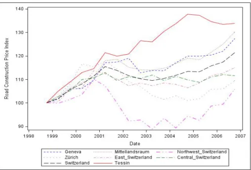
Figure 1: Evolution of the Price Index for Road Construction
revision of the Cartel Act in Switzerland entered in force with direct sanctions.10During this period,
called hereafter the cartel period, all firms active in the road construction sector participated to the cartel, and they rigged all contracts for road construction without exception. Therefore, the Ticino cartel is certainly one of the most severe bid-rigging cartel, also called all-inclusive cartel because all firms participated to rig every contract. It is also an excellent case to study collusion and to test how well detection methods perform.
Close to the end of the cartel, local politicians went to COMCO because they began to suspect prices to be exaggerated. COMCO investigated the prices for road construction, and found that the price index for road construction was significantly higher in Ticino. In fact, as the price index for the rest of Switzerland decreased, the price index for Ticino continued rising in 2002, as depicted on figure 1.11 Finally, the bid-rigging cartel denounced itself in order to benefit immunity until April 2005.
The cartel convention was a written document, and instituted weekly mandatory meeting, at which all firms active in the road construction sector participated. The cartel convention sanctioned absence to these meetings without valid and legitimate reasons, and punished absent firms by
pos-10For COMCO decision, see Strassenbel¨age Tessin (LPC 2008-1, pp. 85-112) 11Source: Swiss Federal Statistical Office.
sible loss of future contracts. In practice, it is unknown if such punishment took e↵ectively place. In each meeting, firms had to announce every new construction contract from public procurement authorities as every other private construction contract above 20’000 CHF. During these meetings, firms discussed contract allocation among them and the bids to submit.
The cartel convention defined di↵erent criteria to allocate new construction contracts. As first criterion, the free capacity of a participant firm was preponderant in the allocation mechanism. Second, the location of the contract work played also a crucial role in the allocation mechanism among participants, especially for contracts below 500’000 CHF. Third, firms considered also the specialization of the participants to allocate contracts. Fourth, the convention privileged participants first invited by private actors to estimate a quotation considering the other criteria. 12 The final
decision of contract allocation was adopted by a majority. In case of divergence, firms vote in secret, except firms involved in litigation.
The Ticino bid rigging cartel never used side-payments, and is therefore a weak cartel (seeMcAfee and McMillan, 1992, for the definition of a weak and a strong cartel). Following Pesendorfer (2000),
two elements allow a weak cartel to achieve efficiency as a strong cartel. First, there must be a lot of contracts to allocate every year within the cartel members. As we can see from table 2, the high number of contracts meets this first condition, with a total of 175 public contracts for the years 1999 to 2004.
Second, a Ranking Mechanism, as described byPesendorfer (2000), should allocate contract among
cartel members. In the Ticino cartel, the cartel convention played the role of the Ranking Mechanism described byPesendorfer (2000). It forced cartel members to reveal their true preferences,
systemati-cally controlled by the allocation criteria of the cartel convention, in order to avoid adverse selection problem. In fact, the cartel convention on its own searched to determine the bidder with the lowest cost for a specific contract in order to maximize theex ante payo↵ of the cartel.
After allocating contracts between cartel members, firms discussed prices. For public contracts,
12Estimating a quotation causes costs which are not recoverable if another firm wins the contract. To avoid such sunk
costs, the convention stipulated that the firm who first announced a private contract had the priority on this contract. It fostered also the announcement of contracts because private contracts are more difficult to observe than public contracts.
all involved firms had to calculate their bids before the meeting. The cartel member, chosen con-sidering all criteria, revealed his price. All participants discussed then the revealed price, and they determined together the best price to submit for the designated winner and the cover bids. Involved participants could not renounce to submit a bid in public tenders; the convention made them submit a bid, respectively a cover bid.
COMCO did not investigate how the cartel members determined the price for the designated winner. However, it is likely that they should have used a rule or any other mechanism to determine relatively quickly the price for the designated winner. In fact, without such a rule, discussions about price could linger too much. One rule could be the following one: the designated winner revealed his price and if the price was not exaggerated, he could submit the bid to this revealed price. Another rule could be that every member revealed their prices and then they calculated the arithmetic mean of all prices; the price of the designated winner could be this arithmetic mean.
If other cartel members had calculated a cheaper bid than the one determined in the discussion, they inflated their bids by some factor to ensure that the designated cartel member would win the contract. The convention stipulates that submitted cover bids should be calculated and justifiable for each position on the bidding documentation provided by procurement agencies. Moreover, cover bids should be high enough relative to the winning bid so that they would not be considered by procurement agencies ensuring the rewarding of the contract to the designated winner.
At the end of the cartel, prices dropped significantly: they were suddenly 25%-30% cheaper than engineer estimates13. It is interesting to note that engineers progressively endogenized the higher cartel price, as proposed by Harrington and Chen (2006). Thus, this observation is an indication
to use with caution engineer estimates to normalize the bids to obtain the dependent variable for econometric estimations.
COMCO condemned all involved firms rendering the decision in 2007 but did not pronounce sanctions against them because the involved firms ceased illegal conducts before April 2005, date to which the revised Federal Act on Cartels entered in force with a sanction regime after a transition
phase from 2004. 14 Because the Ticino road construction cartel was discovered before this date
and because the cartel stopped illicit infringements before the final transitory date of April 2005, COMCO did not sanction the involved firms. If they had been sanctioned, they would have paid a roughly CHF 30 mio penalty.
COMCO defined the relevant market as the market for road construction and pavement in Can-ton Ticino with an upstream market for asphalt pavement material, which plays a strategic role on the road construction and pavement industry. Asphalt pavement material constitutes of 95% of ag-gregates and 5% of asphalt or bitumen and is a crucial input for covering and pavement works. It has to be heated at a mixing plant in order to be mixed and transported quickly to the contract location to cover the road before getting cold. Market specialists say that the duration of asphalt once mixed is comprised between one hour and one hour and half; it is then possible to be operational in a radius of 50-80 km from the production mixing plant.
Because its importance in pavement works and the necessity to transport it heated, pavement material is typically a strategic input. This influences the market structure: firms try to integrate vertically their production process by owning an asphalt mixing plant (see table 9 in Appendix, firm 3, 4, 5 and 6). Because the infrastructure for an asphalt mixing plant is important and expensive, small and local road construction firms try to join their e↵ort in vertical integration by owning com-monly asphalt production plants. In our case, twelve road construction firms own the two biggest asphalt production plants with a capacity of 80% of the overall asphalt production market in Ticino. This cross-ownership on the upstream market conditions the downstream market structure and put serious entry barriers for new competitors because the convention included a clause foreclosing the road construction market: it was forbidden to sell asphalt or other inputs for road construction to third firm not involved in the convention.15 Then, the costs to enter the market were prohibitive because any new entrant should build its own mixing plant. Second, the disciplinary e↵ect of mixing plants was real and enormous. Defecting to the cartel, respectively not taking part to the convention could have raised important difficulties for a single firm considering that asphalt may account for
50% to 80% of the price for pavement works.
3.1 Data
In the rest of this section, we discuss the data for the Ticino case. First, we present some summary statistics. Second, we explain the variables used in the econometric estimation. Specifically, we detail how we construct the variablesdistance and capacity. We use these variables as proxies for the firm
real costs in order to estimate the reduced-form of the bid function in the following sections. Note also that other proxies exist to determine the bid function of each firm i as, for example, the wage of workers, the cost for capital, the price of intermediary inputs (which play a central role in road construction), the taxes paid by the firm. The frequent use of the capacity and the distance in the bid function may be explained for practical reasons: they are simple to be observed and constructed.
Summary Statistics
Table 4 recapitulates briefly the database for the Ticino case. Altogether, the database contains 334 contracts from 1995 to April 2006. However, we have only the records of the tender opening for 238 contracts mainly from the year 1999 to 2006. Therefore, we can identify 1381 submitted bids mainly for the cartel and post cartel period. The tender process follows a first-sealed bid auction, and the tender opening means that at a fixed date, announced by the procurement procedure, public officials open the sealed bids received from the submitting firms. Then, they write the price for each bid and the name of the bidders on a record. This record allows us to have basic information on the contract and on the firms, like the contract location, bidders’ identity and location, prices for each bid.
Table 2 presents the amount of contracts in CHF tendered per year. For the years 1995, 1996 and 2006, we do not have all the contracts publicly tendered. However, we do have all public contracts for the years 1997 to 2005 and we observe important variations of the amount tendered, especially between the years 1997 to 2001. There is a maximal di↵erence of 23 million between the years 1998 and 1999 representing 45% of the maximal amount tendered per year. Major and regular contracts tendered each two years explain these di↵erences.
Table 1: General Descriptive Statistics
Number of tenders 334
Number of submitted bids 2179
Number of tenders with details 238
Number of identified bids 1381
Number of identified bids from individual firm 1100 Number of identified bids from consortia 281 Number of winning bids from individual firms 148
Number of winning bids from consortia 90
Table 2: Tenders per year
Year Contracts Amount
1995 7 16’365’378.95 1996 18 15’881’311.40 1997 50 42’929’902.85 1998 36 28’802’066.70 1999 28 51’896’534.75 2000 27 31’479’500.25 2001 24 46’762’575.10 2002 30 38’713’586.60 2003 21 38’985’740.80 2004 45 35’282’493.70 2005 35 20’926’231.70 2006 14 19’079’459.70 Total 334 387’104’782.50
The sample is characterized by a very high degree of frequent interaction among the same firms. In total, we record 24 firms in the sample but only 17 firms regularly submitted bids for covering and pavement works in Ticino. Table 3 describes the number of bids per tenders for the period from 1995 to 2006. The modus is 4 bids, the mean is 6.5 bids and the median is 6 bids. Note that the number of bids does not necessarily equal the number of bidders because of the possibility for firms to build a consortium.16
Table 3: Bids Distribution
Number of bids 2 3 4 5 6 7 8 9 10 11 12 13 Total
Number of tenders 13 31 53 37 42 44 33 30 18 15 10 8 334
The Bids
In the econometric estimations, we take as dependent variable the natural logarithm of all submitted bids LNBIDitfor all firm i and for all contract t. It is worthy to note, that, in contrast to the literature (seePorter and Zona, 1993, 1999; Pesendorfer, 2000; Bajari and Ye, 2003; Aryal and Gabrielli, 2013),
we do not normalize the bids through the engineer estimates of each contract. First, we possess only a few engineer estimates. Second, engineers endogenized gradually the increase in price, caused by the cartel, exactly as predicted byHarrington and Chen (2006). Indeed, after the breakdown of the
cartel, prices fell 30% under those engineer estimates. Therefore, we would not recommend to use them in our case. But, because we do not standardize the submitted bids, we estimate the regression in the next section with robust variance clustered by firms to take account for heterogeneity.
The Distance
A larger distance between firms and contract location increases the costs, other things being equal, and a rational firm should submit a higher bid in a distant location and a lower bid in a closer location. Therefore, the distance should have a positive impact on the bid function of all firm i.
16A consortium is a joint bidding or a business combination: two bidders or more submit jointly a bid and execute the
Usually, the literature confirms this positive relationship.
We use the number of kilometres calculated from Google Map between the contract location and the firm place, which is the location indicated on the official record of the tender opening.17 Note
also that thedistance changes, if the bid is submitted from the headquarters or from a firm subsidiary.
Then, we add 1 for all observations in kilometre to exclude 0 in order to take the logarithmic of the kilometres.18 The variabledistance is LDISTit= ln(kmit+ 1) for all firm i and for all contract t.
The construction of the distance raises some issues. First, some contracts have two di↵erent lo-cations. We calculate the distance in kilometres for both locations and compute a simple mean for the value of thedistance per firm i. Furthermore, some contracts are provided every two years and
concern principally maintenance works in a particular region of Canton Ticino. We took then the three most important locations situated in the designated region considering the importance of the road network, and we compute again a simple mean for thedistance.19
Second, the address of the firm may not correspond with the exact location of the operation center of the firm. We assume that the firm address, gathered from the official records of the tender opening, corresponds with the nearest operation center for each firm. We cannot verify this information but usually both locations correspond. Third, even if the distance between the operation center and the contract location matters, the distance from the mixing plant to the contract location matters as well. We have no information about the location where firms buy their inputs. Finally, note that the
distance may capture other e↵ects like proximity to the market or to procurement agencies. The Capacity of firms
The assumption for thecapacity is the same for the distance: A firm with a full own capacity engaged
in current contracts should submit a higher bid (if it submits one at all) compared to a firm with a greater free capacity. A firm with few contracts won should submit aggressive bids to win contracts
17Note that we also construct a variable for the travelling time based on Google, and we find the same qualitative results
for the regression in the next section.
18Kilometres equal zero if the contract location is in the same place than the firm location.
19We asked native people from Ticino to determine the three most important locations for the road network in a
in order to fill its order backlog.
Capacity of firms is usually measured in the literature as the volume of contracts won from the beginning of the year until contract t divided by the volume of contracts won during the entire year. Unfortunately, such a measure of the capacity appears inappropriate for our case, since some contracts last two years and not just one year in our data. Thus, the volume of contracts won by each firm i fluctuate significantly per year. Nevertheless, we attempt to construct the capacity for one year, as proposed by the literature, and we find insignificant estimates. We extend thecapacity on
two years, and we find again no significant results. Intuitively, the strong fluctuating income for each firm suggests to calculate thecapacity in a di↵erent way, taking account for the dynamic evolution of the contract volume won per firm.
In this paper, we calculate capacity by summing the contracts won for each firm i and for each
contract t. The value of the contracts won is discounted for all firms i by 10% for each month except from 15th July to 15th August and from 15th December to 15th January. These periods are known as vacation period for the construction industry and the activity is paused or significantly reduced. This depreciation of 10% represents the amount of work completed by firms for each month. Once we calculate the sum of the discounted value of all contracts won for all firms i, we divide each observation for thecapacity by the firm average turnover per year as stated in the COMCO
decision.20. Consequently, thecapacity used in the regression varies from 0 to value over 1, because
the firm turnover fluctuates strongly over the year. Since we do not know the identity of the bidders before January 1999, we cannot observe the capacity. Therefore, we assume that all firms start in
January 1999 with a capacity equal to the half of its average turnover per year. The first observation for the capacity variable for all firms i takes the value of 0.5. We denote it CAPitfor all firms i at the time of contract t. Note also that we exclude the year 2004 for the cartel period because we do not have precise information about the date for 20% of the contracts. The whole cartel period sample, used in the regression in the next section, contains all tenders from 1999 to 2003.
Another problem rises from the fact that we observe only a portion of the market and not the
overall market. In fact, firm turnovers, observed in the COMCO decision, constitute about 60% to 80% of the market volume. In order to have a perfect measure of the capacity variable, we should ask firms to give us a list of all contracts completed per year. If such demand is realistic during an investigation, it seems however unrealistic during anex ante analysis. So, if the official records of the tender opening are insufficient to construct the capacity variable, then this restriction may certainly compromise the use of the method proposed byBajari and Ye (2003) during an ex ante analysis to
screen for collusion. However, as presented in the next section, the capacity variable CAPitprovides good and coherent results.
Strategic Interaction Variables
We create two variables to take account for the strategic interaction between firms. The first variable is the minimal distance among rivals, noted LMDISTit for each firm i at contract t. We expect that the minimal distance among rivals a↵ects positively the bid of firm i. The intuition is the following: if firm i knows that all its rivals are very distant from the contract location, it might raise its bid because it assumes that competition softens. The second variable is the minimal used capacity among rivals, noted MCAPitfor each firm i at contract t. We expect that the minimal capacity among rivals a↵ects positively the bid of firm i. The intuition is the same as for the minimal distance among rivals. If firm i knows that all potential rivals have full capacity engaged in di↵erent contracts, it might raise its bid because competition for the contract will be less fierce.
Consortium
Consortium raises a next concern. Each consortium is a business combination of multiple firms (in general 2 or 3 firms). Usually, a consortium is organized for one contract, but, in our case, we find regularly the same consortia composed by the same set of firms. So, we identify these regular consortia with an identification number as for the individual firms. We give to these regular consortia the identification numbers from 21 to 26. Note also we give the value of 0 for irregular and occasional consortia.
Moreover, we consider uniquely the minimum value of the firms in the consortium to determine the cost variables. This is justified for two reasons: first the convention stipulates this mechanism of the minimum value in order to allocate contracts between di↵erent consortia. Second, the purpose of a consortium usually consists of circumventing capacity restrictions or any other disadvantages. Because of this basic economic justification for consortium, the cost variables of the consortium solely take the minimum value of the costs from firms jointed in the consortium. Table 4 provides basic descriptive statistics for the cartel and post cartel period.
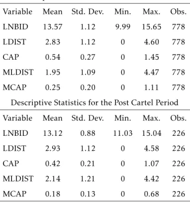
Table 4: Summary of Descriptive Statistics Descriptive Statistics for the Cartel Period
Variable Mean Std. Dev. Min. Max. Obs.
LNBID 13.57 1.12 9.99 15.65 778
LDIST 2.83 1.12 0 4.60 778
CAP 0.54 0.27 0 1.45 778
MLDIST 1.95 1.09 0 4.47 778
MCAP 0.25 0.20 0 1.11 778
Descriptive Statistics for the Post Cartel Period
Variable Mean Std. Dev. Min. Max. Obs.
LNBID 13.12 0.88 11.03 15.04 226
LDIST 2.93 1.12 0 4.58 226
CAP 0.42 0.21 0 1.07 226
MLDIST 2.14 1.21 0 4.42 226
4 Estimating the Bidding Function
As explained in section 2, it is convenient to use a regression analysis in order to test for the condi-tional independence and for the exchangeability of the bids. The related papers in the literature gen-erally estimate a panel model to analyse the structural relationship between the observable covariates
z and the bids (see Porter and Zona, 1993, 1999; Pesendorfer, 2000; Bajari and Ye, 2003; Jakobsson, 2007; Chotibhongs and Arditi, 2012a,b; Aryal and Gabrielli, 2013). Then, we formulate the following panel
model:
yit= xit0 + fit0↵ + "it. (9) In this equation, xitinclude K estimators, and fit0↵ capture the individual fixed e↵ects including a constant term, where i is the subscript for firms and t for contracts. yitis the logarithm of the bids, submitted by firm i for contract t.
In our case, the exogenous variables xit are the cost variables presented in the previous sec-tion, namely the distance (LDISTit), the capacity (CAPit), and the strategic interaction variables (LMDISTit and MCAPit). If LDISTit and CAPit vary for all firms i and for all contract t, each
LMDISTit and MCAPit solely take two values per contract t. For example, the nearest bidder’s
LMDISTittakes for contract t the value of the second nearest bidder for contract t, but for all other bidders (excluding the nearest bidder) LMDISTittakes the value of the nearest bidder for contract t. Note also that these cost variables are solely proxies for the firm real costs. Again, because we repli-cate in this paper the detection method, proposed byBajari and Ye (2003), we consider the functional
reduced-form of the bid function and the cost variables as given. Dummies for contracts (↵t) and for firms ( i) capture the fixed e↵ects.
Based on these cost variables and fixed e↵ects, we estimate the following panel equation, with robust variance clustered by firms:
Empirical Results
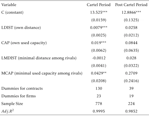
Table 5 reports the estimation of the previous equation for the cartel period and the post cartel pe-riod. For the cartel period, we use in the estimation 130 dummies for contracts (↵t), and 23 dummies for firms ( i). We have a total of 778 observations and 158 regressors.
The estimated coefficients for the distance (LDISTit), the capacity (CAPit), and the minimal
ca-pacity (MCAPit) used among rivals are positive and significant. These results are coherent with the expected behaviour of firms in a competitive environment. If, all things being equal, LDISTitof firm
i increases by 1%, it raises firm i’s bid by 0.79%. The same yields for the firm capacity: if firm i’s CAPit engaged in previous contracts increases, all things being equal, then firm i submits a higher bid. This consistent result also supports the construction of the variable CAPit, discussed in the previous section.
Turning to the strategic interaction variables, we find that the minimal distance among rivals is not significant. However, the minimal used capacity among rivals (MCAPit) is significant and has even a stronger positive e↵ect on firm i’s bid than the own used capacity. Intuitively, if firm i knows that the other firms have already a high capacity engaged in other contracts, it submits a higher bid assuming that competition is soften, because the other firms have too much capacity used to bid aggressively. The fixed e↵ects for contracts (↵t) and for firms ( i) are also significant. Moreover, we notice that the R2 is very high. This can be common for a panel model, and also implies that the
reduced-form of the bid function explains almost all variation observed in the bids. If we retrieve the fixed e↵ects for contracts (↵t), the Adj.R2decreases to 0.3534. To sum up, all these results rather depict a behaviour fitting a competitive environment, although the estimations are made for the cartel period.
For the post cartel period, we use a total of 63 regressors including 39 dummies for contracts (↵t), and 19 dummies for firms ( i). With 224 observations, we have 3.5 time fewer observations than the cartel period sample. All variables are insignificant in the estimation of equation 10. Moreover, we notice that the standard deviation for all variables is roughly 10 times higher than for the cartel pe-riod. This means that the estimators are imprecise, and this phenomenon explains, at least partially,
why the estimators are insignificant. The small sample size and the transition phase, from a cartel to a more competitive equilibrium, may explain this inaccurate estimation. Thus, even if we replicate the econometric tests on the post cartel sample for comparison purpose, we must interpret them with a certain caution. Finally, the R2is again very high, although all variables are insignificant. This
suggests that the high number of dummies compared to the sample size explains mostly the high R2.
Again, R2shrinks to 0.2922 without the fixed e↵ects for contracts (↵t).
Table 5: OLS Estimation for the Reduced-Form Bid Function
Variable Cartel Period Post Cartel Period
C (constant) 13.525*** 12.8866***
(0.0159) (0.1325)
LDIST (own distance) 0.0079*** 0.0258
(0.0025) (0.0212)
CAP (own used capacity) 0.019*** 0.0844
(0.0062) (0.0635)
LMDIST (minimal distance among rivals) -0.0012 0.028
(0.0041) (0.0322)
MCAP (minimal used capacity among rivals) 0.0429** 0.2709
(0.0208) (0.2416)
Dummies for contracts 130 39
Dummies for firms 23 19
Sample Size 778 224
Adj.R2 0.9995 0.9852
5 Testing for collusion
In this section, we implement the tests for the conditional independence and for the exchangeability of the bids. In order to implement these two econometric tests, we estimate the same equation as equation 10 but we allow coefficients to vary across firms i. This is necessary if we want to implement the test of the exchangeability of the bids. All tests presented hereafter are based on the following panel equation:
LBIDit= 0+ i+ ↵t+ 1,iLDISTi,t+ 2,iCAPi,t+ 3,iLMDISTi,t+ 4,iMCAPi,t+ ✏it. (11) Note also that in the rest of this section, we present results not only for a standard risk level of 5%, but also for a risk level of 10%. As explained in the introduction, we might have a problem of false negative results. This means that the tests do not reject the null hypothesis of competition in favour of the alternative hypothesis of collusion, although they should reject it because of the bid-rigging cartel. Then, a simple way to analyse this problem of false negative results is to raise the test risk level at 10%. Because, this implies logically to raise the risk of false positive results, we would not recommend to raise it in other cases, especially in an ex ante screening activity. However, our
case is special, and because we have a perfect information on the Ticino bid-rigging cartel, we cannot make any mistakes, if we reject the null hypothesis of competition for the cartel period. To sum up, presenting the results for a risk level at 10% allows us to discuss the sensitivity of the tests.
5.1 Test for the Conditional Independence
After estimating the equation 11, we test if the residuals of firms i and j are correlated. If the resid-uals are uncorrelated between firms i and j, their bids are independent conditional on the observed cost variables and the fixed e↵ects included in the regression. However, if we find that residuals are correlated, bids are not independent: we can reject the null hypothesis of competition, depicted by the Nash equilibrium of the asymmetric procurement model. Formally, the null hypothesis is the following:
where ⇢ij is the Pearson correlation coefficient. We perform the test only if there is at least five pairwise observations for a pair of firms. This means that both firms submit simultaneously a bid for five contracts. If r is the coefficient of correlation calculated from the data and n the number of pairwise observation for each pair (where n 5), we apply the following Fisher Z transformation:
Z = 1
2ln 1 + r
1 r, (13)
which is approximatively normal with
µZ=12ln1 + ⇢1 ⇢ and Z =p 1
n 3 (14)
If we normalize Z in order to obtain the standard normal distribution, we have
z = (Z µZ)pn 3, (15)
where µZ = 0 under the null hypothesis, i. e. ⇢ = 0. The test statistic is then Zpn 3.
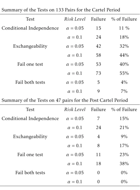
For the cartel period, we test 133 pairs presented in table 10 in appendix and we reject the null hypothesis at 5% risk level for 15 pairs, at 10% for 24 pairs. The failure proportion is 11% and 18%, respectively. This result is surprising because it suggests that false negative results are considerable. For the post cartel period, we apply the test on 47 pairs presented in table 11 in appendix; 7 pairs fail the test at 5% risk level, 24 pairs at 10%. The failure proportion is 15% and 21%, respectively. This result is confusing because we find slightly more rejection for the post cartel period than for the cartel period. We would have expected the contrary.
5.2 Test for the Exchangeability
The test for the exchangeability of the bids examines if the coefficients estimated in equation 11 are identical between firms. If they are identical, it means that firms react in the same way based on their own costs. In other words, if we permute the costs of firm i with the costs of firm j, then firm i should submit the same bids as firm j. The null hypothesis of competition specifies that the estimated coefficients of firm i do not di↵er from those of firm j. Formally, the null hypothesis for the exchangeability of the bids is the following:
The test is implemented with the following F-statistic
F =(SSRC SSRU)/J
SSRU/(N k) , (17)
which has an F-distribution with parameters (J, N-k) under the null hypothesis, where J is the num-ber of constraints, N the sample size and k the numnum-ber of regressors.
Again, we implement the test solely on pairs of firms, which bid simultaneously at least for five common contracts, respectively with five pairwise observations for each pair. Table 14 in appendix shows the results for 133 pairs. We find that 42 pairs fail the test at 5% risk level and 58 at 10%. The failure proportion is 32% and 44%, respectively. Failures are more important for pairs with fewer observations. The pairs failing the test at 5% have on average 14 pairwise observation, whereas the pairs passing the test have on average 19 pairwise observations.
Then, we test the exchangeability of the bids for the post cartel period. Table 15 in appendix recapitulates the results for 47 pairs of firm. We find that 4 pairs fail the test at 5% risk level and 8 at 10%. The failure proportion is 9% and 17%, respectively.
To sum up, the test for the exchangeability of bids performs better, because it produces fewer false negative results than the test for the conditional independence. Yet, false negative results remain important because more than half of the pairs pass the test, although they should fail. Furthermore, we also observe that the number of failure decreases for the post cartel period. This result is logical because, if the test of exchangeability is correct, we expect that the number of failure decreases in a more competitive market.
If we consider the simultaneous application of both tests at 5% risk level, we find that only 5 pairs fail both tests and 53 pairs fail solely one of them. The failure proportion is 4% and 40%, respectively. At 10% risk level, we find that solely 9 pairs fail both tests and 73 pairs fail one of them. The failure proportion is 7% and 55%, respectively. This result suggests that the failure of one test should be sufficient to raise concerns about the existence of bid-rigging cartel. We discuss it deeper in section 7.
Table 6: Summary of Econometric Tests Summary of the Tests on 133 Pairs for the Cartel Period
Test Risk Level Failure % of Failure
Conditional Independence ↵ = 0.05 15 11 %
↵ = 0.1 24 18%
Exchangeability ↵ = 0.05 42 32%
↵ = 0.1 58 44%
Fail one test ↵ = 0.05 53 40%
↵ = 0.1 73 55%
Fail both tests ↵ = 0.05 5 4%
↵ = 0.1 9 7%
Summary of the Tests on 47 pairs for the Post Cartel Period Test Risk Level Failure % of Failure
Conditional Independence ↵ = 0.05 7 15%
↵ = 0.1 24 21%
Exchangeability ↵ = 0.05 4 9%
↵ = 0.1 8 17%
Fail one test ↵ = 0.05 11 23%
↵ = 0.1 18 38%
Fail both tests ↵ = 0.05 0 0%
6 Robustness Analysis
In the previous section, we test for collusion, and we find a high number of false negative results. These results are erroneous, and they contradict the existence of the Ticino bid-rigging cartel. Thus, we examine in this section, if these results are robust only for the cartel period with two di↵erent sub-samples, composed by cover bids. We use cover bids, because they are less informative than the cartel winning bids; Cover bids are, by definition, fake. Then, we could assume that cover bids are less connected with costs than the cartel winning bids. If this is true, we should therefore find more rejection for these two sub-samples, respectively fewer false negative results.
For the first sub-sample, we consider only the pairwise observation, when firm i and firm j submit both cover bids. We call this first sub-sample, theindirect cover bids sample, because neither firm i
nor firm j wins the contract, but they both submit a cover bid in favour of a third cartel member. Hence, the indirect cover bids contain solely cover bids, excluding all winning bids. Note also that, for the cartel period, all winning bids are the lowest submitted bids for each contract.
For the second sub-sample, we consider solely the pairwise observation, where firm i wins the contract and firm j submit a cover bid. We call this sub-sample the direct cover bids sample, because firm i wins the contract whereas firm j submit a cover bid; respectively firm j direct cover firm i. Note also that the second sub-sample contains all pairwise observation excluded in the first sample, so that the addition of the two sub-samples produces the whole sample.
In the following, we implement the test for the conditional independence and for the exchange-ability of the bids on the indirect cover bids sample. Then, we apply solely the conditional indepen-dence test on the direct cover bids sample.
6.1 Testing Collusion for the Indirect Cover Bids Sample 6.1.1 The Conditional Independence Test
By analyzing the residuals of the regression from equation 11 for the cartel period, we find immedi-ately that the residuals of the winning bids are significantly lower than the residuals of the cover bids.
Table 7 shows that the simple mean is -0.0277 for the winning bids and 0.0055 for the cover bids, with a standard deviation of 0.0187 and 0.0164, respectively. To sum up, the residuals of the winning bids are in average 5 times lower than those of the cover bids with an approximative equal spread. In other words, the residuals of the cover bids first order stochastically dominates the residuals of the winning bids. This important di↵erence between the empirical distribution of both residuals may influence notably the estimated Pearson correlation coefficient. Then, it might be interesting to verify whether the results for the conditional independence test change, if we consider solely the residuals for the cover bids.
Table 7: Descriptive Statistics according to the Type of Residuals
Mean St. Dev. Min Max N L. Quartile Median U. Quartile
Resid. Cover Bids 0.0055 0.0164 -0.0473 0.0763 649 -0.0045 0.0042 0.0151
Resid. Winning Bids -0.0277 0.0187 -0.0711 0.0262 129 -0.042 -0.0281 -0.0158
To implement the test, we use the same residuals of equation 11 from section 4, but we suppress the residuals of the winning bids for each contract. We calculate the Pearson correlation coefficient and use, as in section 4, the Fisher transformation. Table 12 in appendix recapitulates the results. The tests reject the null hypothesis for 14 pairs at 5% risk level and for 25 pairs at 10%; the failure proportion is 15% and 26%, respectively. If we consider the pairs composed solely by individual firms, we reduce the sample on 83 pairs, and we obtain 10 rejections at 5% risk level, 21 rejections at 10%; In sum, we notice approximatively the same proportion of failure (12% and 25%) for individual firms. Moreover, the proportion of failures for the conditional independence test does not change with this sub-sample. As for the whole sample of the cartel period, we find again too many false negative results.
6.1.2 The Test for the Exchangeability of the Bids
pairwise observations for the two firms; this means if both firms participate at least for five common contracts, each firm submitting five cover bids in favour of a third cartel member.
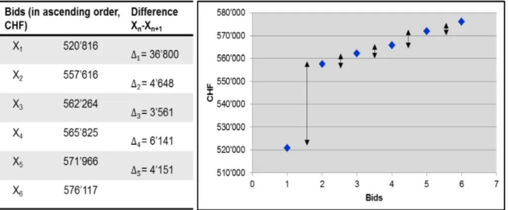
The motivation to reduce the sample solely on the indirect cover bids is di↵erent from the reason mentioned for the conditional independence test. Looking at figure 2 drawn fromImhof et al. (2015),
we observe an important gap between the winning bids and the cover bids. In fact, the average gap is roughly 5%. However, we remark immediately from figure 2, that the gaps are smaller between the cover bids. This pattern is observable for the majority of the contracts during the cartel period (seeImhof , 2017). Therefore, if cover bids are very close, and if costs are di↵erent among firms, then the estimated coefficients of equation 11 could be di↵erent across firms. In other words, we expect a greater number of failure for this test.
Figure 2: Typical Cover Bidding Mechanism in Ticino
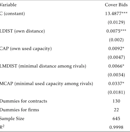
Table 8 presents the results for the estimation of equation 11 for the indirect covers bids sample. We note that all variables are positive and significant. The distance has virtually the same e↵ect on the bids as shown for the whole cartel period sample: if, all things being equal, the distance of firm i increases to 1%, it raises firm i’s bid by 0.75%. The own used capacity and the minimal used capacity among rivals have a weaker e↵ect on the bids compared to the whole cartel period sample. They are significant only at 10% risk level. We observe interestingly that the minimal distance among rivals is positive and significant at 10% risk level, whereas it is not significant for the whole cartel period sample. The R-squared is also higher. This is certainly explained by the fact that we have fewer observations and almost the same number of regressors. The results of this regression may surprise:
we would have expected to find less consistency with a rational economic behaviour for the indirect cover bids sample. On the contrary, these results suggest that costs explain somehow the cover bids.
Table 8: OLS Estimation of the Reduced-Form Bid Function for the Cover Bids
Variable Cover Bids
C (constant) 13.4877***
(0.0129)
LDIST (own distance) 0.0075***
(0.002)
CAP (own used capacity) 0.0092*
(0.0047)
LMDIST (minimal distance among rivals) 0.0066*
(0.0034) MCAP (minimal used capacity among rivals) 0.0337* (0.0181)
Dummies for contracts 130
Dummies for firms 22
Sample Size 645
R2 0.9998
Where ***, **, * denote significance level at 1, 5, 10 percent level.
Table 16 in appendix presents the results of the tests for 96 pairs. We find that 19 pairs fail at 5% risk level and 28 at 10%. The failure proportion is 20% and 29%, respectively. Then, the portion of pairs, failing the test of exchangeability for the indirect cover bids sample, decreases by 12% and 15%, respectively.
This result surprises again because we would have expected to find more failures for this sub-sample. We explain this result by two causes, which are mutually non-exclusive. First, the costs for the cover bids do not di↵er as much as we could have expected. However, if they di↵er, they enter in a symmetric way in the firm bid function. Second, firms gathered together each week, and they discussed extensively the bids for public contracts, as it is stated in the cartel convention. Regular discussions could explain why costs, if they di↵er, enter in a symmetric way in the firm bid function.
We would have expected the contrary. In any case, this result confirms again the high number of false negative results, observed for the whole cartel period sample.
6.2 Testing Collusion for the Direct Cover Bids Sample
We turn now to test the conditional independence test on the direct cover bids sample. We are interested to analyse the residuals between the winning bids and the losing bids, where firm i wins the contract and firm j submit a cover bid. In fact, we postulate that a significant di↵erence between the two types of residuals, as observed with simple descriptive statistics in 7, may produce a strong correlation pattern.
Again, we calculate the Pearson correlation coefficient and use, as in section 4, the Fisher trans-formation. Table 13 in appendix presents the results. We consider again all pairs with at least 5 simultaneous bids, and we retain 35 pairs for the direct cover bids sub-sample. As expected, 24 pairs reject the null hypothesis at 5% risk level, 28 at 10%. The proportion of failing pairs is 69% and 80%, respectively; we find also strong negative correlation for the failing pairs. The test produces substantially fewer false negative results for the direct cover bids sample, and is consistent with the Ticino bid-rigging cartel.
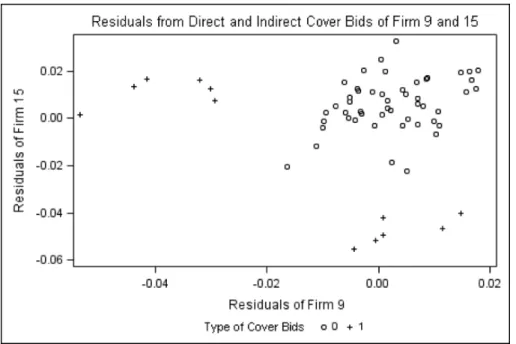
Intuitively, we can explain this phenomenon on the basis of figure 3 depicting the pairwise residu-als of firms 9 and 15 for the whole cartel period sample, where both firms bid for the same contracts. We di↵erentiate the type of cover bids between indirect and direct cover bids, represented on the figure by circles and crosses, respectively.
In the previous section, we found that pair (9,15) had 62 simultaneous bids with a non significant correlation of 0.0595; the pair does not fail the conditional independence test. Considering only the indirect cover bids (circles on the figure), we find 50 simultaneous (indirect) cover bids with a significant positive correlation of 0.3498. However, if we restrict the sample solely on the direct cover bids (crosses on the figure), we observe 12 simultaneous bids and a significant negative correlation of 0.8866.
corre-lation from the direct cover bid sample. Because of this antagonistic e↵ect, the correlation for the whole cartel period sample is not significant. The pair passes the test, whereas we expect it to fail. This phenomenon is common for many pairs, which pass successfully the test of the conditional in-dependence for the whole cartel period sample. This result indicates that the test of the conditional independence is better designated to detect bilateral agreement and not an all-inclusive bid-rigging cartel, as the Ticino case. We discuss this result in the next section.
Figure 3: Pairwise Residuals of firm 9 and 15
7 Policy Implication for Competition Agencies
In this section, we discuss the high number of false negative results. Then, we address the ques-tion of classifying a pair of firms as potential cartel, if the pair fails solely one test or if it fails both tests. In other words, is the failure of one test a sufficient condition to alarm competition agencies? Second, we compare the method proposed byBajari and Ye (2003) with a di↵erent method devel-oped byImhof et al. (2015) to screen for bid-rigging cartels. From this comparison, we deduce some
recommendations for competition agencies.
an error of type II: the test should reject the null hypothesis but it does not reject it whereas the null hypothesis is definitively false. In our case, the null hypothesis is competition for both econometric tests, and we do not reject it for a large percentage of pairs for both tests, although we implement the tests for the cartel period. Again, we remind the reader that the bid-rigging cartel in Ticino rigged all contracts for the cartel period, and all firms participated to the bid-rigging cartel, without exception. Certainly, we study with the Ticino case a bid-rigging cartel of the worst kind. Therefore, considering the severity of the bid-rigging cartel, how can we explain the high number of false negative results observed?
Considering the high number of false negative results, we suggest first a data-related explana-tion. The data may be imprecise, or the construction of the variables incorrect. However, incorrect data or miss-constructed variables should rather contribute to reject the null hypothesis of competi-tion. It would be very unlikely to have incorrect data or miss-constructed variables fitting the strong hypotheses of Nash equilibrium in a first-sealed bid asymmetric procurement model. Moreover, the results of the panel estimations contradict also this conjecture of data imprecision: if data or variables were incorrect, it would be again very unlikely to find that firms bid following a rational economical behaviour. Finally, one can attempt to put in question the assumed reduced-form of the bid function. Yet, the literature has well established the empirical identification for the reduced-form of the bid function used in this paper (seePorter and Zona, 1993, 1999; Pesendorfer, 2000; Bajari and Ye, 2003; Jakobsson, 2007; Chotibhongs and Arditi, 2012a,b; Aryal and Gabrielli, 2013). In any case, if the data
used in this paper is insufficiently accurate, it means that the official records of the tender opening are not sufficient to construct the variables for the bid function. Then, the data requirement to meet is too high, if a competition agency wants to implementex ante the econometric tests proposed by Bajari and Ye (2003), based only on the official records of the tender opening.
After excluding the date-related explanations, we turn now to discuss model-related causes for those false negative results. First, if firms pass the two econometric tests, although they collude on all contracts, it might imply that they manage to pass through the tests proposed by Bajari and Ye
Figure 4: The Evolution of the Coefficient of Variation
model might also encompass collusion. Indeed, if cartel members scale their bids with a common factor, the assumptions underlying the competitive model proposed byBajari and Ye (2003) remains
non-violated: the cartel can pass through the tests.
However, we can exclude in our case this bid scaling phenomenon. Imhof (2017) presents the
application of simple statistical screens to detect collusion for the Ticino case and finds that simple statistical screens capture well the impact of the bid-rigging cartel. Figure 4 drawn fromImhof (2017)
depicts the evolution of the coefficient of variation, where the two vertical lines delimit the cartel period. The di↵erence between the cartel and the post cartel period is eye-catching: the coefficient of variation is significantly lower during the cartel period indicating the existence of a bid-rigging cartel, as predicted by the variance screen (seeImhof et al., 2015; Imhof , 2017).
Yet, simple screens function only if cartel members do not scale their bids. If they scale their bids, it is impossible to detect collusion with simple screens as shown byImhof (2017). In sum, we
can exclude the bid scaling phenomenon for the Ticino case. Therefore, it seems realistic to consider that a cartel can manage to pass through the tests proposed byBajari and Ye (2003) without scaling
their bids. This result is somehow pessimistic towards the method proposed byBajari and Ye (2003).