Energy-loss magnetic chiral dichroism (EMCD): Magnetic chiral dichroism in the electron microscope

Papers in this section are based on submissions to the MRS Symposium Proceedings that were selected by Symposium Organizers as the outstanding paper. Upon selection, authors are invited to submit their research results to Journal of Materials Research. These papers are subject to the same peer review and editorial standards as all other JMR papers. This is another way by which the Materials Research Society recognizes high quality papers presented at its meetings.

Review

Energy-loss magnetic chiral dichroism (EMCD):

Magnetic chiral dichroism in the electron microscope

S. Rubinoa)

Institute for Solid State Physics, Vienna University of Technology, Vienna A-1040, Austria; and Department of Engineering, Uppsala University, Uppsala S-751 21, Sweden

P. Schattschneider

Institute for Solid State Physics, Vienna University of Technology, Vienna A-1040, Austria; and Service Centre for TEM, Vienna University of Technology, Vienna A-1040, Austria

M. Stöger-Pollach

Service Centre for TEM, Vienna University of Technology, Vienna A-1040, Austria

C. Hébert

SB-CIME Station 12, EPFL, Lausanne, Switzerland

J. Rusz

Department of Physics, Uppsala University, Uppsala S-751 21, Sweden; and Institute of Physics, Academy of Sciences of the Czech Republic, Prague CZ-18221, Czech Republic

L. Calmels, B. Warot-Fonrose, F. Houdellier, and V. Serin

Nanomaterieaux Group, CEMES-CNRS, FR-31400 Toulouse, France

P. Novak

Institute of Physics, Academy of Sciences of the Czech Republic, Prague CZ-18221, Czech Republic (Received 3 April 2008; accepted 17 July 2008)

A new technique called energy-loss magnetic chiral dichroism (EMCD) has recently been developed [P. Schattschneider, et al. Nature 441, 486 (2006)] to measure magnetic circular dichroism in the transmission electron microscope (TEM) with a spatial resolution of 10 nm. This novel technique is the TEM counterpart of x-ray magnetic circular dichroism, which is widely used for the characterization of magnetic materials with synchrotron radiation. In this paper we describe several experimental methods that can be used to measure the EMCD signal [P. Schattschneider, et al. Nature 441, 486 (2006); C. Hébert, et al. Ultramicroscopy 108(3), 277 (2008); B. Warot-Fonrose, et al. Ultramicroscopy 108(5), 393 (2008); L. Calmels, et al. Phys. Rev. B 76, 060409 (2007); P. van Aken, et al. Microsc. Microanal. 13(3), 426 (2007)] and give a review of the recent improvements of this new investigation tool. The dependence of the EMCD on several experimental conditions (such as thickness, relative orientation of beam and sample, collection and convergence angle) is investigated in the transition metals iron, cobalt, and nickel. Different scattering geometries are illustrated; their advantages and disadvantages are detailed, together with current limitations. The next realistic perspectives of this technique consist of measuring atomic specific magnetic moments, using suitable spin and orbital sum rules, [L. Calmels, et al. Phys. Rev. B 76, 060409 (2007); J. Rusz, et al. Phys. Rev. B 76,060408 (2007)] with a resolution down to 2 to 3 nm.

a)

Address all correspondence to this author. e-mail: stefanorubino@yahoo.it

This paper was selected as the Outstanding Symposium Paper for the 2007 MRS Fall Meeting Symposium C Proceedings, Vol. 1026E.

I. INTRODUCTION

The transmission electron microscope (TEM) is a powerful investigation instrument for materials science with a scope comprising tomographic reconstruction of cells, materials characterization, crystal structure and de-fects, microelectronic devices, and spintronics, to name a few. It is one of the most successful applications derived from de Broglie hypothesis on the wave-particle duality of matter, i.e., that all particles also have a wave nature. Electrons, with a wavelength much shorter than visible light, have allowed the study of the properties of matter at the nanometer and subnanometer scale; it should be mentioned that the synchrotron-based x-ray microscopy has also seen a tremendous improvement in spatial reso-lution, recently reaching the 25 nm limit.1

In the last decades, the TEM capabilities have been augmented by the introduction of electron energy loss spectrometry (EELS): by measuring the energy lost by the electron beam while passing through a sample it is possible to obtain additional information as atoms are ionized or plasmons, interband and intraband transitions are excited (microanalysis). Moreover, the fine structure of such spectra reveals information about the density of states (DoS) above the Fermi energy, which is strongly related to the chemical bonds involving the excited atom. The x-ray counterpart of EELS is x-ray absorp-tion spectroscopy (XAS), from which similar spectra are obtained when measuring the intensity reduction of an x-ray beam passing through a sample and exciting the same transitions.

One of the characteristics of light that apparently breaks the so far complete similarity between x-ray and electrons is the possibility to produce (and experiment with) polarized photons. In this contest, one phenomenon has been out of the reach of the TEM community for a long time: dichroism, i.e., the property of certain mate-rials that their absorption spectra are a function of the polarization of the incident radiation (when this is visible light, the material appears to have two different colors when seen from different directions, hence the name). Dichroism can be linear or circular (depending on the polarization of the photons) and natural or magnetic (de-pending on the origin—crystallographic or magnetic—of the sample anisotropy).

X-ray magnetic chiral dichroism (XMCD), after its discovery 20 years ago,2has become a routine technique in many synchrotron beam lines to study element-specific magnetic properties of ferromagnetic materials and, via sum rules, to separate spin and orbital contribu-tions to the magnetization.3,4Whereas it is not difficult to show that linear dichroism in the TEM corresponds to angular-resolved EELS,5,6 it was assumed that spin-polarized electron beams would be needed for the TEM equivalent of XMCD. However, a careful examination

and comparison of the scattering cross section for EELS and XAS shows that a simple, commercially available TEM equipped with a spectrometer is all that is needed to study MCD with electron scattering.7–12

In this paper we present a review of the principles involved in EMCD experiments, together with a detailed description of the techniques used and a few illustrative examples.

II. THEORY

A. Chirality in XMCD experiments

The physical origin of XMCD can be understood when calculating the transition probabilities of an electron from a core state to a free state above the Fermi energy. When a circularly polarized photon with helicity parallel to the magnetization is absorbed, the target atom acquires a quantum of angular momentum. This means that only transitions which obey the ⌬J ⳱ ±1 selection rule are allowed. We now focus on the L2,3edges of 3d magnetic

transition metals, which correspond to electronic transi-tions from the 2p core states to unoccupied s or d valence states. Contributions corresponding to p→ s transitions can be neglected with respect to those that correspond to p→ d transitions.13

Photons with +1 and −1 helicity, respectively, induce the additional selection rule⌬m ⳱ 1 and ⌬m ⳱ −1 and force transitions to final states that may be differently occupied. The resulting spectral lines will then have dif-ferent intensities, thereby explaining how polarization af-fects the shape of the final absorption spectrum. The 2p core hole states, which give rise to the L2,3 edge, are

divided into 2p1/2 states (L2 edge) and 2p3/2 states (L3

edge) that have different energies. The fine structure of each of these two edges depends on their different tran-sition probabilities and on the DoS for majority and mi-nority spin unoccupied valence states.14 XMCD sum rules can be used to obtain the spin and orbital magnetic moments from experimental spectra.3,4

In XAS the spectral intensity IXASis given by:

IXAS= ␣␻

冱

ⱍ

具

典

ⱍ

2 _{␦共E + E}

i − Ef兲 , (1)

where ␣ is a factor that does not depend on the photon angular frequency␻, |i〉 and |f 〉 are the initial and final states of the target electron with energies Ei and Ef

re-spectively, e is the polarization vector of the photon and

r is the position operator. In the case of left or right

circular polarization we can simply substitute e with

e1 ± i e2, where e1 is perpendicular to e2 with a ±␲/2

phase shift. The more general case of elliptical polari-zation can always be reduced to a superposition of cir-cular and linear polarization. For example, a generic phase shift⌬␸ (represented as e1+ e

i⌬␸

e2) can be

de-composed into sin⌬␸(e1+ i e2) + 2(1 − sin⌬␸) e3where

B. Chirality in electron scattering

When a single diffracted beam is involved, the spectral intensity IEELSfor electron scattering is given, in dipole

approximation, by:

I_EELS= ␣⬘共k_fⲐk_i兲

冱

ⱍ

具

典

ⱍ

the fast electron wave and q⳱ kf− kiis the wave vector

transfer. The sum over the matrix elements is called the dynamic form factor (DFF). Equations (1) and (2) show that the wave vector transfer q plays the same role in electron scattering as the photon polarization vector e in XAS. The fact that the similarity between EELS and XAS is not only formal has been demonstrated in q-resolved EELS experiments.5,6In this case, the term an-isotropy is customarily used instead of linear dichroism. In analogy to the previous section, we now consider an experimental geometry that involves two incident waves with wave vectors k1 and k2. If the experimental

con-figuration is such that these incident waves correspond to two perpendicular momentum transfer vectors q1and q2

with a ±␲/2 phase shift, we can replace q in Eq. (2) by (q1

± i q2). The spectral intensity is then given by:

IEELS= ␣⬘共kfⲐki兲1Ⲑq 4

冱

ⱍ

具

典

ⱍ

冱

共

ⱍ

具

典

ⱍ

ⱍ

_具

典

ⱍ

Ⳳ 2Im兵

具

典具

典

兲

(3) where the first two terms are the DFFs corresponding to the scattering of each of the incident waves (k1 and

k₂ with modulus ki), and the interference term

⌺i,f〈f |q1⭈r|i〉〈i|q2⭈r|f 〉 ␦(E + Ei − Ef) is the so-called

mixed dynamic form factor (MDFF).15In a more general

experimental configuration where, for example, the vec-tors q1and q2are not perpendicular, the interference term

also depends on the real part of the MDFF. In cubic systems it is, however, possible to demonstrate that the real part of the MDFF is proportional to (q1⭈q2), while its

imaginary part, which does not vanish for magnetic ma-terials, is proportional to (q1 × q2).

12,16

The physical foundations of the equivalence between XAS and EELS can be traced back to the electric field at the target atomic site. In an XAS experiment, polarized photons are directly responsible for the electric field E whose direction is defined by the polarization vector e. An electric field E can also be associated to the fast electron of a TEM beam. The direction of this field is given by q. In both cases, this electric field is the driving agent of the ionization process caused by the absorption of a real photon in XMCD and a virtual photon in EMCD.

C. Scattering geometry

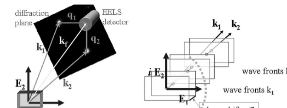
Four conditions are required to perform an EMCD experiment: (i) two electron beams must exist so that two simultaneous momentum transfers can occur; (ii) the two momentum transfers must not be parallel (perpendicular in the ideal case); (iii) they must not be in phase (with a phase shift of␲/2 being the optimal condition); and (iv) we must be able to change the helicity of the excitation. These conditions are summarized in Fig. 1.

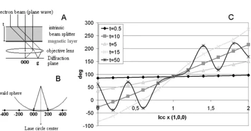
Several methods have been proposed to obtain two electron beams in the TEM; however, in this article we restrict our discussion to the so-called intrinsic method, where a crystalline sample is used to split the beam via Bragg scattering. When the electron wave enters the crystal, it undergoes a decomposition into Bloch waves, whose amplitude and phase can be calculated within the framework of the Bloch theory16,17

and can be controlled by setting the boundary conditions (namely beam tilt and specimen thickness) to appropriate values, as shown in Fig. 2.

FIG. 1. Scattering geometry for the EMCD experiment. Two incident plane waves, with wave vectors k1and k2, produce each an oscillating

electric field (E1and E2) at the atom. An aperture is then placed in the diffraction plane to select the final scattering direction (kf) so that q1and

q2are perpendicular to each other. When the phase shift between the two incident waves is set to␲/2 the total electric field at the atomic site is

The advantage of the intrinsic method is that it pro-vides two simultaneous momentum transfers (two Bragg scattered beams being excited) and a way to control their phase shift (which is identical for all atoms at the same depth and occupying the same elementary cell position). Therefore, the intrinsic method fulfills conditions 1 and 3 at the same time. Condition 2 can be reached by a suit-able selection of the scattering direction kf, placing either

the objective aperture (OA) or the spectrometer entrance aperture (SEA) on the Thales circle in the diffraction plane. This also provides a simple way to change the helicity (condition 4) as illustrated in Fig. 3.

An alternative way to switch from one helicity of the excitation to the other would be to modify the boundary conditions to change the phase shift. Figure 2 shows for instance that the phase shift for a 15 nm thick sample

changes from␲/2 for Laue circle center (Lcc) (1,0,0) to −␲/2 (which corresponds to the opposite helicity) for Lcc (0,0,0). The model presented in Fig. 2 is an oversimpli-fication of the reality. A better description of the EMCD experiment must take into account the fact that the ion-ization process can occur at any depth inside the crystal. It must also consider the fact that both the incoming and outgoing beams are diffracted as Bloch waves inside the crystal.18All these improvements can be included using the dynamical diffraction theory framework from which the spectral intensity can be expressed as16:

I_EELS= ␣⬘共k_fⲐk_i兲

冱

冱

冱

具

qjr兲ⱍi

典具

典

i − Ef兲 .

(4)

FIG. 2. (a) In the intrinsic method a crystalline specimen is used as beam splitter. The sample can be seen as composed of two parts: a first layer of thickness t that sets the chirality of the electron beam and the target magnetic layer where the ionization process occurs. (b) The Laue circle center (Lcc) is a convenient way to indicate the tilt of the incoming electron beam with respect to the crystal. It is defined as the projection, on

the diffraction plane, of the center of the Ewald’s sphere, i.e., the sphere having the incident kivector as its radius (diffraction points are strongly

excited only if they lay close to the surface of the Ewald’s sphere). (c) Plot of the phase shift between the direct and the first diffracted beam (2,0,0 of face-centered cubic nickel) as a function of the tilt of the incident beam and for different values of the thickness (in nm) of the sample.

FIG. 3. Chirality of the electron excitation in an EMCD experiment. The Thales circle is constructed in the diffraction plane by taking as its diameter the segment connecting the 000 and g spot. We obtain the TEM equivalent of circular polarization when the OA (or the SEA) is located

on the Thales circle in such a way that |q1|⳱ |q2| and when their phase shift is set to␲/2. The helicity of the virtual photon absorbed in the EMCD

The index j( j⬘) is used to label the incident (outgoing) Bloch wave with wave vector transfer qj (qj⬘). The

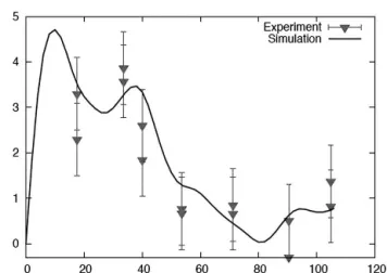
co-efficient T ( j, j⬘,t) depends on the thickness of the sample and is obtained by summing over the successive unit cells in the crystal. The AA*( j,j⬘) are the products of the Bloch wave coefficients. The vectors u give the position of the N atoms contained inside the unit cell. Examples of the thickness dependence of the EMCD signal are shown in Ref. 16 and Fig. 4.

III. EXPERIMENT

We have applied the procedure detailed previously, shifting the detector at the two symmetric positions of the diffraction plane, to demonstrate the feasibility of EMCD experiments and the soundness of the physics behind this technique. The dichroic signal has been measured in a 10 nm thick Fe layer grown on a GaAs substrate previously characterized with standard XMCD measurements.7 Other magnetic materials have been investigated, as shown in Fig. 5. A FEI Tecnai F20-FEGTEM S-Twin with a Gatan Imaging Filter (GIF; Vienna, Austria) was used in these experiments.

The SEA of the GIF is used to select kfin the

diffrac-tion pattern. The signal is produced by the entire illumi-nated area, which can be reduced by use of a selected area aperture (SAA). When parallel illumination is used the measured intensity is reduced, as a large part of the electron beam is blocked by the aperture. The SAA de-termines the spatial resolution (no better than 100 nm in this configuration). The diffraction pattern is electroni-cally shifted with respect to the SEA, and the two spectra are acquired under identical conditions.

When the OA is used to select kf, the TEM can be

operated in normal (image) mode. The detected signal now originates from an area given by the projection of the SEA on the image. The dimensions of this area are set by the magnification and can be reduced to the nano-meter range. Again, when parallel illumination is used this area is only a small fraction of the illuminated area and much of the beam intensity is blocked by the aper-tures. Another disadvantage is that the TEM has to be switched between image and diffraction mode and that the OA has to be shifted manually to invert the helicity (this affects the precision with which kfis selected). In

both cases, the intensity of the signal is low and acqui-sition times of the order of several minutes have to be used.

A. LACDIF (Large-Angle Convergent DIFfraction) and the q-E diagram

So far, conditions as close as possible to parallel illu-mination and pointlike detector were used; that is, the convergence and collection angles were chosen as small as possible. The reason for this is twofold: it is easier to calculate the spectra under this approximation, and any deviation from this condition reduces the circularity of the exciting radiation and thus the dichroic signal. Re-ferring to Fig. 3 (left) and neglecting all other Bragg spots, it can be seen that, for example, a nonzero collec-tion angle means a range of possible values for kf (area

inside the +1 and −1 circles) and therefore for q1and q2.

Only the point at the center of the +1 or −1 circle is on the Thales circle; for all other points q1 and q2 are not

perpendicular and the excitation acquires a linearly po-larized component (as it was previously shown for a generic⌬␸) reducing the dichroic content of the signal. The next step is then to observe the evolution of the dichroic signal as we deviate from these conditions. In particular, it is of interest to know if the reduction in dichroic content can be compensated for by an increase of the spectral intensity. For this purpose the LACDIF setup9,19,20was used to obtain a diffraction pattern in the image plane (see Fig. 6). LACDIF is a defocused method, which allows us to obtain diffraction patterns in the image plane. This is achieved by focusing the elec-tron beam on the specimen, which is then moved upward from the eucentric position by a distance z. The cone of illumination will select on the sample an area of radius ␣z, which can be reduced to approximately 5 nm without a Cs corrector. EMCD spectra can then be acquired with the detector shift method. Since no SAA is used, the intensity of the signal is up to 2 orders of magnitude higher and the spatial resolution is given by the cone of illumination (∼20 nm radius in Ref. 20).

In combination with this modified geometry, a q-E diagram (Fig. 6) also provides a means to acquire the spectra with opposite chirality in one acquisition, thus reducing the negative effect of specimen and beam drift

FIG. 4. Thickness dependence of EMCD in hcp Co. Relative

peak-to-peak difference at the L3edge (779 eV) for the two symmetric

positions on the Thales circle, with g⳱ (1,0,0) and Lcc ⳱ (1/2,0,0).

The simulations were calculated combining density functional theory

and dynamical diffraction theory.16 _{The triangles are experimental}

or other instabilities. To obtain such a diagram, it is necessary to rotate the diffraction pattern (using, for ex-ample, a rotational holder) so that the 000 and g spots lay on the energy-dispersive axis of the spectrometer (here called x axis). In spectroscopy mode, the GIF integrates the image entering the SEA (in this case a diffraction pattern) in the x direction and then disperses the electron according to the energy they have lost. Each pixel of the image obtained displays the intensity of the electron scat-tering for a particular value of the energy lost and of the scattering angle in the y direction (normally this image is further integrated in the y direction to give the energy loss spectrum). The range of integration in the qx

dimen-sion is different for points with different qy and is

determined by the SEA and the camera length (given by the magnification and the defocus distance z in the LACDIF setup). In the case of Fig. 6 the 0.6 mm SEA is as big as the Thales circle. The integration range ⌬qx⳱ √(g

2

/4 − q2y) would reduce to a pixel for the

posi-tions with opposite helicity on the Thales circle. It should be noted that LACDIF and the q-E diagram can be used separately.

B. CBED

In the LACDIF setup, it was shown that relatively large convergence angles still yield a significant dichroic signal. A CBED configuration was then tried to further

FIG. 5. EMCD measurements on metallic iron, cobalt, and nickel. The iron sample was a 10 nm layer epitaxially grown on a GaAs substrate; the

Co and Ni samples were electropolished single crystals. The percentage variation of the average intensity at the L3peak is indicated.

FIG. 6. LACDIF and q-E diagram setup. (a) The electron beam (solid lines) is focused on the specimen, obtaining a sharp spot in the image plane (and a disk in the diffraction plane, not shown); when the specimen is lifted upward from the eucentric position Bragg spots appear in the image plane (dotted lines); (b) the diffraction pattern is rotated so that the g vector is parallel to the x axis of the spectrometer; when the GIF switches

from image to spectroscopy mode the diffraction pattern is integrated in the qxdirection, with the x axis now replaced by the energy loss axis.

We obtain a qyversus E diagram where each horizontal line correspond to an energy loss spectrum with a particular value of qyand integrated

over a certain range of qx. The SEA can be used to select the integration range; (c) line profiles of the q-E diagram for the qyvalues of the opposite

improve the possible spatial resolution without sacrific-ing spectral intensity. Similarly to LACDIF, the beam is focused on the specimen, but then the microscope is switched to diffraction mode. A diffraction pattern with large disks will appear. The size of these disks (i.e., the convergence angle) is defined by the condenser apertures and is about 2 to 3 mrad in our experiment (Fig. 7). The specimen (hexagonal close-packed Co, the 3 axes nota-tion is used) is tilted 5.18° away from the [001] zone axis to excite the (110) systematic row. Since for every pos-sible kfwe now have a combination of circular and linear

polarization, we have no reason to expect that the maxi-mum of the dichroic signal is at the Thales circle, espe-cially if all significant Bragg spots are taken into account. Indeed simulations21have shown that for a three-beam case (i.e., Lcc ⳱ 000) the maximum of dichroism is obtained for the positions depicted in Fig. 7. It is also possible to show that a large collection angle improves the signal-to-noise ratio.21 The other Bragg spots are only weakly excited and can thus be neglected even if they happen to be on the projection of the SEA (as it is the case of the 010 spot).

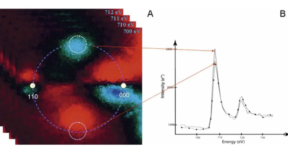
C. Energy spectroscopic diffraction

An alternative approach to EMCD experiments can be obtained by using the energy spectroscopic diffraction or imaging (ESD or ESI) techniques.9

In ESD, the diffrac-tion pattern is projected on the GIF and a series of energy filtered images is acquired, scanning the L2,3edge. From

the data cube thus obtained, the dichroic signal can be extracted in two ways (Fig. 8). We can take the energy-filtered image of the diffraction pattern recorded for the

energy loss corresponding to the L3 (or L2) peak. To

improve the signal-to-noise ratio, all images correspond-ing to the L3edge can be summed up. The line

connect-ing the 000 and the diffracted spot is used as a mirror plane to change the value of every pixel to the one of the pixel with same x and opposite y coordinate. We subtract this mirrored image from the original image, and we obtain, point by point, the dichroic signal as difference between the L3peak values of spectra with same qx but

opposite qy. For the case of only two Bragg spots, the

maximum is expected to be at the opposite points in the Thales circle.

Alternatively, we can imagine placing a virtual aper-ture in the same position in every image of the recorded diffraction pattern and measure the intensity falling within this aperture as function of the energy loss at which the image was recorded. The plot thus obtained is nothing else than the energy-loss spectrum that would have been recorded with that particular scattering angle (i.e., with the SEA in the place of the virtual aperture). Extracting the corresponding spectrum from the opposite position on the Thales circle gives us an EMCD meas-urement.

For ESI, it is an image of the sample that is projected on the GIF and then an energy filtered series is started. It should be noted that in this case the OA is needed to select kf.

D. Detection of magnetic phase transitions with EMCD

Since EMCD depends on the magnetization of the sample, it is possible to detect changes in the magnetic

FIG. 7. CBED configuration. The Co crystal is tilted in the (−1,1,0) direction from the [001] zone axis to a three beam case, i.e., with G⳱ (1,1,0)

and −G equally excited. The other Bragg spots are shown for completeness but are weakly excited. The detector shift technique is used without SAA to record spectra from positions with opposite helicities (the gray circles indicate the SEA in such positions). The spatial resolution is given

properties of matter. Monitoring magnetic phase transi-tions of magnetic nanostructures opens fascinating per-spectives for future spintronics applications. We could demonstrate such a phase transition in a crystal of Pr0.5Sr0.5MnO3.

22

This compound is antiferromagnetic below 160 K, paramagnetic above 267 K, and ferromag-netic in the remaining range (Fig. 9). This was confirmed by temperature-dependent EMCD measurements at the Mn L2,3 edge (640 eV). The O K edge (532 eV) was

recorded as well to identify eventual artifacts in the ac-quisition and did not show any dichroic effect, as ex-pected. The signal was obtained from a single crystalline region of 130 nm radius.

IV. CONCLUSIONS

The techniques briefly illustrated here show that it is possible to routinely measure MCD in the TEM with a spatial resolution of 10 nm or better using several complementary methods. Recently, it was also demon-strated10,12

that EMCD sum rules can be applied to de-rive the spin and orbital contributions to the magnetiza-tion of the sample, or at least their ratio (absolute values

are difficult to obtain due to the EMCD dependence on the tilt and thickness of the crystal).

The two main limitations of the EMCD experiment are: (i) the area of interest needs to be a single crystal (with a radius as small as a few nm), which can be oriented in a two- or three-beam configuration; (ii) the magnetic field of the TEM lenses at the specimen loca-tion (1–2 Tesla) is high enough to saturate most of the magnetic samples along the TEM optical axis. Saturation could be avoided by developing a Lorentz-like mode for EMCD, where the objective lens is deactivated.

With better spatial resolution and depth sensitivity than XMCD, EMCD can be a powerful investigation tool, giving important contributions in the study of magnetic properties of interfaces and nanostructures, spin valves, FM-AFM pinning, GMR devices, and spin-tronics.

ACKNOWLEDGMENTS

This research was supported by the European Commission, Contract No. 508971 (CHIRALTEM). We acknowledge J. Hejtmanek for providing the Pr0.5Sr0.5MnO3sample.

FIG. 9. EMCD magnetic phase transition. Pr0.5Sr0.5MnO3is ferromagnetic only within a defined temperature range [figure modified from Ref.

22]. When EMCD measurements are performed with a temperature controlled stage it is possible to detect the change in the magnetic character of the sample from its dichroic signature. For the sake of clarity the differences are enhanced by a factor of 5.

FIG. 8. ESD. (a) A series of energy filtered images of the diffraction pattern of body-centered cubic Fe is acquired with an energy window of

1 eV. The one corresponding to the peak of the L3edge (at 709 eV) is then mirrored with respect to the line connecting the 000 and 110 spot and

then subtracted from itself. The result shown here is a map of the absolute dichroic signal (blue corresponds to a variation of +8% from the average, light red to −8%). (b) a virtual aperture is placed in every image of the series and the signal within that area is integrated. A plot of this integration as a function of the energy loss gives the spectrum for that particular scattering angle.

REFERENCES

1. D.H. Kim, P. Fischer, W. Chao, E. Anderson, M.Y. Im, S.C. Shin, and S.B. Choe: Magnetic soft x-ray microscopy at 15 nm resolu-tion probing nanoscale local magnetic hysteresis. J. Appl. Phys.

99,08H303(2006).

2. G. Schütz, W. Wagner, W. Wilhelm, P. Kienle, R. Zeller, R. Frahm, and G. Materlik: Absorption of circularly polarized x-rays in iron. Phys. Rev. Lett. 58, 737 (1987).

3. B.T. Thole, P. Carra, F. Sette, and G. vander Laan: X-ray circular dichroism as a probe of orbital magnetization. Phys. Rev. Lett. 68, 1943 (1992).

4. C.T. Chen, Y.U. Idzerda, H-J. Lin, N.V. Smith, G. Meigs, E. Chaban, G.H. Ho, E. Pellegrin, and F. Sette: Experimental confirmation of the x-ray magnetic circular dichroism sum rules for iron and cobalt. Phys. Rev. Lett. 75, 152 (1995).

5. A.P. Hitchcock: Near edge electron energy loss spectroscopy: Comparison to x-ray absorption. Jpn. J. Appl. Phys. 32(2), 176 (1993).

6. P. van Aken and S. Lauterbach: Strong magnetic linear dichroism

in Fe L23and O K electron energy-loss near-edge spectra of

an-tiferromagnetic hematite␣-Fe2O3. Phys. Chem. Miner. 30, 469

(2003).

7. P. Schattschneider, S. Rubino, C. Hébert, J. Rusz, J. Kuneš, P. Novak, E. Carlino, M. Fabrizioli, G. Panaccione, and G. Rossi: Experimental proof of circular magnetic dichroism in the electron microscope. Nature 441, 486 (2006).

8. C. Hébert, P. Schattschneider, S. Rubino, P. Novák, J. Rusz, and M. Stöger-Pollach: Magnetic circular dichroism in electron energy loss spectrometry. Ultramicroscopy 108(3), 277 (2008). 9. B. Warot-Fonrose, F. Houdellier, M.J. Hÿtch, L. Calmels,

V. Serin, and E. Snoeck: Mapping inelastic intensities in diffrac-tion patterns of magnetic samples using the energy spectrum im-aging technique. Ultramicroscopy 108(5), 393 (2008).

10. L. Calmels, F. Houdellier, B. Warot-Fonrose, C. Gatel, M.J. Hÿtch, V. Serin, E. Snoeck, and P. Schattschneider: Experi-mental application of sum rules for electron energy loss magnetic chiral dichroism. Phys. Rev. B 76, 060409 (2007).

11. P. van Aken, L. Gu, D. Goll, and G. Schütz: Electron magnetic linear dichroism (EMLD) and electron magnetic circular

dichro-ism (EMCD) in electron energy-loss spectroscopy. Microsc.

Mi-croanal. 13(3), 426 (2007).

12. J. Rusz, O. Eriksson, P. Novák, and P.M. Oppeneer: Sum-rules for electron energy-loss near-edge spectra. Phys. Rev. B 76, 060408 (2007).

13. G. Schütz, R. Wienke, W. Wilhelm, W. Wagner, P. Kienle, R. Zeller, and R. Frahm: Strong spin-dependent absorption at the

L2,3-edges of 5d-impurities in iron. Z. Phys. B 75, 495 (1989).

14. S.W. Lovesey and S.P. Collins: X-Ray Scattering and Absorption

by Magnetic Materials, edited by J. Chikawa, J.R. Helliwell, and

S.W. Lovesey (Clarendon Press, Oxford, 1996), pp. 120–131. 15. H. Kohl and H. Rose: Theory of image formation by inelastically

scattered electrons in the electron microscope. Adv. Electron.

Electron Phys. 65, 173 (1985).

16. J. Rusz, S. Rubino, and P. Schattschneider: First principles theory of chiral dichroism in electron microscopy applied to 3d ferro-magnets. Phys. Rev. B 75, 214425 (2007).

17. A.J.F. Metherell: in Electron Microscopy In Material Science, edited by E. Ruedl and U. Valdrè (CEC, Luxembourg, 1975), pp. 397–552.

18. Y. Kainuma: The theory of Kikuchi patterns. Acta Crystallogr. 8, 247 (1955).

19. J.P. Morniroli, F. Houdellier, C. Roucau, J. Puiggalí, S. Gestí, and A. Redjaïmia: LACDIF, a new electron diffraction technique ob-tained with the LACBED configuration and a Cs corrector: Com-parison with electron precession. Ultramicroscopy 108(2), 100 (2008).

20. P. Schattschneider, C. Hébert, S. Rubino, M. Stöger-Pollach, J. Rusz, and P. Novák: Magnetic circular dichroism in EELS: Towards 10 nm resolution. Ultramicroscopy 108(5), 433 (2008). 21. J. Verbeeck, C. Hébert, S. Rubino, P. Novák, J. Rusz, F. Houdellier, C. Gatel, and P. Schattschneider: Optimal aperture sizes and po-sitions for EMCD experiments. Ultramicroscopy 108(9), 865 (2008).

22. J. Hejtmánek, E. Pollert, Z. Jirák, D. Sedmidubský, A. Strejc, A. Maignan, C. Martin, V. Hardy, R. Kužel, and Y. Tomioka:

Magnetism and transport in Pr1−xSrxMnO3single crystals (0.48艋