Path planning for mobile robots in the real
world
Handling multiple objectives, hierarchical structures and partial
information
Doctoral Dissertation submitted to the
Faculty of Informatics of the Università della Svizzera italiana in partial fulfillment of the requirements for the degree of
Doctor of Philosophy
presented by
Jérôme Guzzi
under the supervision of
Prof. Luca Maria Gambardella and Dr. Alessandro Giusti
Dissertation Committee
Prof. Cesare Alippi Università della Svizzera italiana, Lugano, Switzerland
Prof. Francesco Mondada École polytechnique fédérale de Lausanne, Switzerland
Prof. Evanthia Papadopoulou Università della Svizzera italiana, Lugano, Switzerland
Prof. Domenico Sorrenti Università di Milano-Bicocca, Italy
Dissertation accepted on 12 July 2018
Research Advisor Co-Advisor
Prof. Luca Maria Gambardella Dr. Alessandro Giusti
PhD Program Director PhD Program Director
Prof. Walter Binder Prof. Olaf Schenk
I certify that except where due acknowledgement has been given, the work presented in this thesis is that of the author alone; the work has not been submit-ted previously, in whole or in part, to qualify for any other academic award; and the content of the thesis is the result of work which has been carried out since the official commencement date of the approved research program.
Jérôme Guzzi
Lugano, 12 July 2018
Abstract
Autonomous robots in real-world environments face a number of challenges even to accomplish apparently simple tasks like moving to a given location. We present four realistic scenarios in which robot navigation takes into account partial infor-mation, hierarchical structures, and multiple objectives. We start by discussing navigation in indoor environments shared with people, where routes are charac-terized by effort, risk, and social impact. Next, we improve navigation by com-puting optimal trajectories and implementing human-friendly local navigation behaviors. Finally, we move to outdoor environments, where robots rely on un-certain traversability estimations and need to account for the risk of getting stuck or having to change route.
Acknowledgements
I would like to thank my supervisors Luca Maria Gambardella and Alessandro Giusti for their invaluable support, and all people that traveled with me on my journey in robotics research: Gabriele Scascighini who kicked off the adven-ture, Andrea Rizzoli and Alexander Forster who, together with Luca Maria Gam-bardella, welcomed me at IDSIA, Gianni di Caro who supervised the first part of the thesis, and my colleagues Frederick Ducatelle, Eduardo Feo Flushing, Jawad Nagi, Jacopo Banfi, Fang-Lin He, Juan Pablo Rodríguez Gómez, Boris Gromov, and Omar Chavez-Garcia, for their precious help.
This work was partially supported by the Fondazione Informatica per la Pro-mozione della Persona Disabile (FIPPD), the European Union Active and Assisted Living Programme (AAL), and the Swiss National Competence Center for Re-search in Robotics (NCCR-Robotics).
Contents
Contents vii
Introduction 1
1 Path planning in indoor spaces 9
1.1 Introduction . . . 9
1.2 Related Work . . . 10
1.2.1 Spatial representations . . . 10
1.2.2 Rich maps and multi-objective path planning . . . 11
1.2.3 Trajectory planning in social spaces . . . 12
1.3 Model . . . 13 1.3.1 Problem formulation . . . 13 1.3.2 IndoorGML . . . 13 1.3.3 Microscopic attributes . . . 14 1.3.4 Navigation layer . . . 15 1.3.5 Macroscopic attributes . . . 18
1.3.6 Navigation line graph . . . 24
1.3.7 Multi-objective optimization . . . 25
1.4 Experiments . . . 31
1.4.1 Experimental setup . . . 31
1.4.2 Results . . . 33
1.5 Concrete instances . . . 33
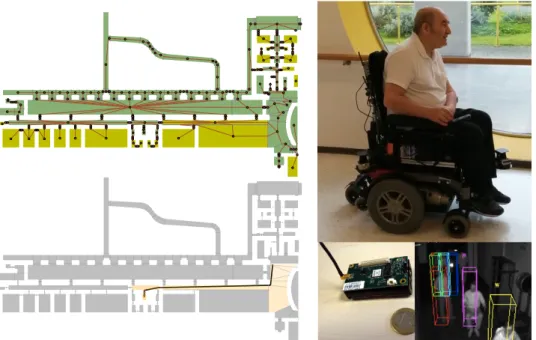
1.5.1 Optimal topological planning for smart wheelchairs . . . . 33
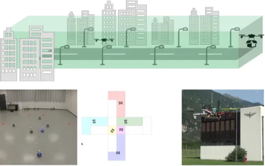
1.5.2 Drones coordination on a flyway . . . 39
1.6 Conclusions and Perspectives . . . 39
2 Optimal trajectory planning in indoor spaces 43 2.1 Introduction . . . 43
2.2 Related Work . . . 44
2.3 Model . . . 45 vii
viii Contents
2.3.1 The jerk along a trajectory as a cost . . . 45
2.3.2 Problem formulation . . . 47
2.3.3 Search space . . . 48
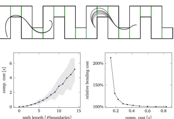
2.3.4 Bending cost optimisation . . . 51
2.3.5 Optimal trajectories in indoor buildings . . . 53
2.3.6 Geometric multi-objective optimization . . . 54
2.4 Experiments . . . 54
2.4.1 Synthetic map . . . 55
2.4.2 Real building map . . . 55
2.4.3 Multi-objective planning example . . . 57
2.4.4 Robot navigation . . . 57
2.5 Conclusions and Perspectives . . . 58
3 Human-friendly local navigation 61 3.1 Introduction . . . 61
3.1.1 Local navigation . . . 61
3.1.2 Human-friendly behavior . . . 62
3.1.3 Emerging collective behaviors . . . 62
3.1.4 Outline . . . 63
3.2 Related Work . . . 64
3.2.1 Local navigation in robotics . . . 64
3.2.2 Local navigation in social sciences . . . 65
3.2.3 Robot behavior acceptance . . . 66
3.3 Model . . . 67
3.3.1 Problem formulation . . . 67
3.3.2 Pedestrian heuristics . . . 67
3.3.3 Application to robot navigation . . . 69
3.4 Comparison with alternative navigation behaviors . . . 73
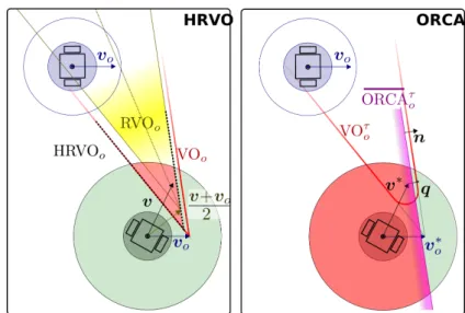
3.4.1 Behaviors based on Reciprocal Velocity Obstacle . . . 73
3.4.2 Comparison with the Human-like behavior . . . 75
3.5 Navigation along a geometrical trajectory . . . 76
3.6 Experimental setup . . . 77
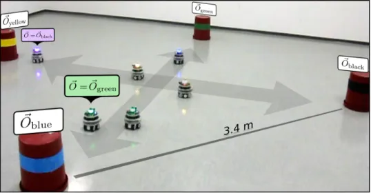
3.6.1 Scenarios . . . 77
3.6.2 Robots and sensing . . . 79
3.6.3 Simulation . . . 80
3.6.4 Implementation of navigation behaviors . . . 80
3.7 Experiments . . . 81
3.7.1 Safety . . . 84
ix Contents
3.7.3 Validation with real robots . . . 85
3.7.4 Scalability . . . 87
3.7.5 Heterogeneous swarms . . . 87
3.7.6 Emerging collective behaviors . . . 88
3.7.7 Trajectory following . . . 92
3.8 Discussion . . . 93
3.9 Conclusions and Perspectives . . . 97
4 Planning with traversability estimations 99 4.1 Introduction . . . 99
4.1.1 Planning according to traversability estimations . . . 100
4.1.2 Risk-aware path planning . . . 101
4.1.3 Resilent path planning . . . 101
4.2 Related work on the Canadian traveller problem . . . 102
4.3 Risk-aware path planning . . . 103
4.3.1 Problem formulation . . . 103
4.3.2 Approximated convex-hull of the Pareto front . . . 105
4.3.3 Experiments . . . 107
4.4 The impact of the estimator quality on the navigation policy . . . 110
4.4.1 Problem formulation . . . 112
4.4.2 Binary traversability classifier . . . 112
4.4.3 Optimal and baseline policies . . . 114
4.4.4 Experimental setup . . . 116
4.4.5 Experimental Results . . . 118
4.4.6 Discussion . . . 124
4.5 Conclusions and Perspectives . . . 124
5 Conclusion 127 5.1 Summary . . . 127
5.2 Looking forward . . . 130
A Publications 133
Introduction
Making a robot solve a simple task is usually a complex exercise for researchers, even without considering the challenge to design and build a working piece of hardware. Complexity arises when we instantiate the robot’s task in the real world, even more so when the robot interacts with people.
In the thesis we focus on a ubiquitous task for autonomous mobile robots: reach a given target position using the robot’s locomotion capabilities. In fact, there are instances of this problem, illustrated in any textbook, that are simple to model and relatively easy to solve, e.g., computing a feasible path given a grid map whose cells are either obstacles or free space. Yet, modeling realistic navi-gation tasks is complex. Simply reaching the target along the shortest possible path is often not enough; instead, we expect the robot to follow a trajectory that satisfies multiple other implicit goals.
As an illustration, let us consider the navigation task that a service robot needs to solve to go somewhere within a city using a map of the road (and sidewalk) network. From our experience as pedestrians, we quickly realize that the robot needs to consider many aspects. The robot should comply with traffic rules and move in a considerate, predictable manner when crossing people along the side-walks. The robot should work well even with maps that are not always accurate; for example, maintenance works may block the access to some sidewalks on a given day. Finally, the robot performance depends on the environment; for ex-ample, the robot may need to avoid direct sunlight to be able to rely on infrared sensors and avoid obstacles; the robot may be equipped with wheels able to over-come small steps but not large ones, and may get stuck on streetcar rails when crossing them at an oblique angle. This scenario describes a complex navigation task.
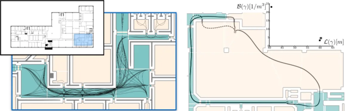
In the thesis, we instantiate and solve navigation and path planning problems in different contexts and different level of abstraction, as illustrated in Figure 1. In Chapter 1, the robot is traveling from one side to the other of a building, fol-lowing a path that requires low effort, has a low risk of accidents, and minimizes discomfort caused to other users (in particular to people). The environment is
2 Contents
Chapter 1 Chapter 2 Chapter 3
Chapter 4
Figure 1. Outline of the thesis. Chapter 1: accounting for many factors, the robot plans the best path and identifies a sequence of cell boundaries to cross (in blue). Chapter 2: the robot chooses an optimal (short, smooth and legible to others) trajectory (blue) across these cell boundaries. Chapter 3: the robot smoothly navigates around people. Chapter 4: the robot now ventures outside in the unstructured world. The robot is not sure if it will be able to traverse a part of rough terrain and decides that is better to take the longer path instead of the shorter but riskier path. At the same time, the robot prefers crossing the river where there are two visible nearby bridges: in case one of them is found to be not traversable, backtracking to the other one will be cheap.
3 Contents
modeled as a set of cells (i.e., a non-regular decomposition of two-dimensional space into polygons) that contain a rich description of their relationship with the robot’s navigation task. We compute a high-level topological route: a sequence of cells to traverse to reach the goal.
In Chapter 2, we go one step further and compute the continuous trajectory that the robot should follow along the high-level route. We consider the case when the robot is a smart wheelchair that has to be comfortable for the user (turn gently and avoid excessive accelerations). Moreover, the robot should account for the presence of other people, and, in particular, make its current goal easy to infer.
In Chapter 3, the robot is following a trajectory across a space crowded with people. Like them, the robot needs to continuously adjust its motion to avoid collisions. In addition, the robot’s motion has to be as human-friendly as possible: in particular, it should strive to conform to the way humans use to navigate. Are humans proceeding along lanes? Then the robot should queue itself and follow the flow.
In Chapter 4, the robot has arrived at the other end of the building and ven-tures outside to navigate in a less structured environment. The robot needs to estimate whether it is able to traverse several stretches of difficult outdoor ter-rain. The estimate is computed by a statistical classifier using incomplete data, which has non-ideal accuracy; the robot, when planning a path, has to take into account the uncertainty in traversability estimates. When the robot arrives in place, it is able to refine the traversability estimates using data from its onboard sensors. The robot implements navigation strategies that are resilient to discover-ies made along the path: in particular a resilient navigation strategy favors paths that offer cheap alternatives should a portion turn out to be not traversable.
When dealing with these issues, we observe three recurrent, connected themes: hierarchical structures, partial information and multiple objectives.
Hierarchical structures A realistic robotic task usually needs to be broken down
to manageable subtasks that interact with each other. A prominent example is given by the first three chapters, where the task of reaching a target point is broken down into three subtasks, which iteratively refine the solution: (1) com-pute a high-level route; (2) comcom-pute a geometric trajectory along the route; (3) avoid dynamic obstacles along the trajectory. The subtasks are related in mul-tiple ways. In direction 1 → 2 → 3, the output of one planner serves as the input (goals or constraints) of the next planner. In the opposite direction, lower level planners serve to model costs. For example, a high-level planner estimates
4 Contents
the effort needed to cross a room with a given occupancy based on the average performance of a local navigation controller in that setting.
Partial information In Chapter 1, we model heterogeneous spatial descriptors:
attributes that may be subjective or objective, personal or general. We assume that, at planning time, information is complete and that the robot will be able to handle dynamic changes along its way, as e.g., in Chapter 3, where we handle unforeseen obstacles that were previously outside of the robot’s view and we show that a reactive navigation policy is a good strategy to cope with them.
In Chapter 4, we deal with partial information in a different context, i.e., un-certain estimates concerning ground traversability. We discuss how the appro-priate way to handle these uncertain estimates within a path-planning problem crucially depends on the consequences of attempting to cross a terrain that is not traversable. In particular, we distinguish the case in which the robot gets irreversibly stuck, and the case in which the robot can backtrack and continue traveling on a different route; we show that each case yields a very different formalization of the path planning problem.
Multiple objectives When framed in realistic contexts, a navigation task
usu-ally requires multiple objectives to be satisfied. In Chapter 1, we introduce the topic through an explicit model. The model derives, from a rich spatial de-scription of navigability, a summary representation defining a few costs that are well suited to address many different scenarios, in particular when people share spaces with robots. In Chapter 2, we interpret some objectives (in particular legibility) as constraints and search for trajectories that are smooth and short. In Chapter 3, we proceed in a different way: one of the objectives (human-friendliness) is satisfied by design through the selection of the navigation be-havior, instead of by explicit optimization. In Chapter 4, we finally link partial information to risk and formulate risk-aware multi-objective path planning prob-lems.
When optimization over multiple objectives is suitable, we assume that we are computing plans for a strategic decision maker (or agent) that sits on top of the planning hierarchy. In Chapters 1 and 2, we compute exact solutions of multi-objective optimization path planning problems over (sparse) navigation graphs, whereas in Chapter 4 we compute approximations because the navigation graphs are too large.
5 Contents
Contributions
In this section I use the singular personal pronoun to clarify my contributions over the state-of-the-art and my own contributions in the collaborative research effort, and to summarize the scientific outcome in terms of publications, project milestones and software releases; the detailed list of scientific publications (Ap-pendix A) and software releases (Ap(Ap-pendix B) are provided as appendices.
Contributions over the state-of-the-art
Chapter 1: Path planning in indoor spaces I propose an extension of a recent standard for indoor maps[89] that adds a rich description of the relation between agents and spaces, with particular focus on robotic navigation. I propose an abstract model to describe planning costs in terms of geometry and environment state; I identify three macroscopic costs that describe many common scenarios both in robotics and in route planning for people.
Mine is the first effort to present a complete pipeline: from deriving a navi-gation graph, to defining and solving a multi-objective path planning problem in these spaces; this pipeline is composed by algorithms that are novel, namely: de-composing the space in few quasi-convex cells well suited for planning; comput-ing the exact Pareto front of the multi-objective problem by iterative application of a state-of-the-art algorithm for the k-th shortest path on a graph[156]. Each of these algorithms solves a specific, narrow problem and therefore represents a minor contribution over the state-of-the-art[88].
Publications We introduced the pipeline for path planning in social spaces using three macroscopic costs (effort, safety risk, and social impact) in a work-shop paper [56]. We elaborated on it to support users with restrained mobility in nursing homes in two project deliverables[53, 54].
Chapter 2: Optimal trajectory planning in indoor spaces I present a novel derivation of the cost associated with the discomfort of following a trajectory sitting on a robotic wheelchair as an intrinsic geometrical property. I use this cost and a parametrization of trajectories as composite Bézier curves, to define a non-linear optimization problem that searches for the trajectory that turns most gently. In this regard, I extend the state-of-the-art [28, 36, 147] in several di-rections: a) my approach can compute a long, complex trajectory that spans a whole building whereas previous work was limited to passing trough a single door; b) my approach adds constraints to increase predictability; c) I propose an effective heuristic to initialize the search; d) I propose a novel method to limit the
6 Contents
dimensionality of the search space without compromising smoothness; e) I de-fine and solve a novel multi-objective problem in the search for short trajectories that turn gently.
Publications We presented our optimal trajectory planner for wheelchairs in a conference paper[55].
Chapter 3: Human-friendly local navigation I present the first application to robotics of a state-of-the-art heuristic [103] used in social sciences to describe the navigation of pedestrians [105]. I compare it with two known algorithms for local robot navigation[14, 135], introducing new benchmarks for individual and group navigation performance; it is the first systematic comparison between reactive navigation algorithms with a large scale simulation campaign and real-robot tests. Moreover, I explore novel ideas on multi-real-robot implicit coordination, such as using artificial emotions to modulate the collective behavior.
Publications We described the extension of the pedestrian heuristic to ro-botics in a conference paper [60]. We compared it with other collision avoid-ance algorithms [14, 135] in conference paper [61]. Similar to what observed in crowds [66, 104], local navigation rules let macroscopic behaviors emerge in groups of robots, which we investigated in a conference paper[59]. We dis-cussed how to improve navigation using artificial emotions in two conference papers[57, 58].
Chapter 4: Planning with traversability estimations In a joint effort with
col-leagues, I developed the first application of machine learning to estimate the traversability of a portion of an heightmap, which inspires the definition of path planning problems. In this framework, my specific contribution was to formalize risk-aware multi-objective path planning on maps with uncertain traversability estimations and develop a novel algorithm to approximate its solution; this is an incremental contribution over state-of-the-art multi-objective planners[35].
I also propose the first large scale investigation on a question that has not been tackled yet in the literature, namely: how does the quality of traversability estimations impact the performance of the navigation policies for the (very well-known) Canadian traveller problem[8, 113]?
Publications We present the complete pipeline — from estimation of ter-rain traversability to risk-aware multi-objective path planning — in a journal paper [26]. We discussed the impact of traversability estimation on the cost of navigation policies in a workshop paper[62].
7 Contents
Own contributions to collaborative research
A very large part of the work presented in the thesis originate from my direct con-tribution. Nonetheless, scientific research is not an individual effort and I could profit from many contributions from other researchers. I briefly go through each chapter to separate my contributions from the contributions of colleagues; the important contribution of the advisor (Prof. Luca Gambardella) and co-advisors (Prof. Gianni di Caro and Dr. Alessandro Giusti) in all my research activity and research output is always implied; in particular, the advisor and co-advisors ac-tively participated in discussing and suggesting research ideas and assisting in the preparation of research papers.
Path planning in indoor spaces I developed the model, implemented the soft-ware and evaluated the planner performance. For the ALMA project, researchers from SUPSI-DSAN helped to define the attributes to describe social spaces; other partners have provided interfaces for my planner to the localization system, user interface and robotic wheelchair (POLIMI) and to the smart cameras (VCA); site tests were a collaborative effort of all project’s partners. For the DFW project, I implemented the software on the light poles and on the drones with the help of Dr. Eduardo Feo Flushing.
Optimal trajectory planning in indoor spaces I developed the model,
imple-mented all software and evaluated the planner performance. The robot con-troller makes use of the open source ROS framework and the planner uses on open source numerical solvers.
Human-friendly local navigation I adapted the pedestrian navigation model to
robotics, compared it with alternatives, developed a custom simulator for large multi-agent scenarios, implemented the Human-like navigation behavior, and performed all the experiments; Dr. Alessandro Giusti contributed the model for simulating robot cameras. For the comparison, I use third-party, open source implementations of the other algorithms [69, 126]. The biomimetic model for tuning navigation based on artificial emotions is a joint idea of Prof. Gianni di Caro and me.
Planning with traversability estimations The design of the machine learning algorithms and the collection of the dataset in simulation was performed by Dr.
8 Contents
Omar Garcia-Chavez and Dr. Alessandro Giusti. I developed the risk-aware plan-ner; I tested it on real maps and real robots with the help of Dr. Omar Garcia-Chavez and other partners from NCCR Robotics (ETHZ, EPFL and UNI-ZH). I de-signed the analysis of the Canadian traveler problem together with Dr. Alessan-dro Giusti. I implemented the policies, the random graph generators, performed the test and evaluated the results.
Scientific output
During the work that led to this thesis, I published, together with coauthors, 4 papers in major robotics journals (1 in Autonomous Robots, 2 in Robotics and Automation Letters, and 1 in Robotics Automation Magazine) and 13 papers in major robotics conferences: 4 at IROS, 2 at ICRA, 1 at GECCO, 1 at AAMAS, 2 at AAAI, 1 at AVICS, 1 at BIONETICS and 1 at ICSR. I was the responsible for providing mapping and planning services for a ALMA, a large EU AAL project, for DFW, a smaller Swiss CTI project, and for one work package in the search and rescue grand challenge of phase 2 of NCCR-Robotics that provided resilient path planning for ground robots on rough terrain. These efforts resulted in the open source release of 7 software libraries: a pipeline for indoor planning, its application in nursing homes and its extension to coordinate of a fleet of drones; a multi-agent simulator; a ROS package with various reactive navigation policies; a ROS package with a risk-aware path planner; and a library to perform large scale navigation experiments on random maps with uncertain traversability.
Chapter 1
Path planning in indoor spaces
1.1
Introduction
An autonomous robot is traveling towards its destination inside a building. To reach it, the robot will have to traverse several spaces with different character-istics (narrow corridors, slippery floors, crowded halls, dark rooms, steep stairs, and so on). Which one of the many alternative routes should it follow?
In this chapter, we focus on this question starting from the observation that indoor spaces have rich spatial descriptions. Spatial information gives us clues about difficulties and tradeoffs that the robot will face such as: it may fall or get stuck on some floor types; it should avoid private rooms; it may struggle to maintain good localization in dark spaces.
We approach the problem through a bottom-up analysis. We first discuss and model spatial representations that are well suited to encode rich spatial descrip-tions typical of environments shared with people. Then, we extract the most relevant information for a robot to navigate safely, efficiently and in a way that does not hinder people: a generic model that gives rise to a multi-objective path planning problem. Finally, we instantiate the generic problem on two real-world applications: computing appropriate routes for autonomous wheelchairs in nurs-ing homes; coordinate drones along flyways, an outdoor scenario that features a similar spatial structure.
We present a model that lets agents account for rich information about them-selves and their environment, and get a description of several optimal routes (each made of a sequence of cells to traverse) to reach a destination. In the next chapters, we will discuss how to refine the plans: in Chapter 2 we compute the best trajectory that passes through a sequence of cells; in Chapter 3 we study how the robot avoids dynamic obstacles along the route.
10 1.2 Related Work
1.2
Related Work
1.2.1
Spatial representations
When humans describe a scenery, they normally label each part: “here is a grass field, there is a swamp, and in between a river”. To encode this description in a map, we may list pairs of shapes and labels.
Typically shapes attached to different labels may overlap: the grass field and the swamp may be part of a larger flatland area. There are at least two alterna-tives to encode overlapping spatial information. We could use a single generating set of shapes and attach multiple labels to a shape, labeling areas as flatland grass or flatland swamp. Alternatively, we could separate conflicting labels into non-overlapping sets of shapes: a set of shapes would only carry labels about terrain grounds like grass and swamp, while another set would carry labels about terrain shape like flatland.
The second alternative, which we adopt in this chapter, is common in geo-graphical information science, for which a family of (vectorial) multilayered[9, 158] formats (foremost the Geographic Markup Language, GML) contains tagged features linked to arbitrary polygonal shapes (also referred as cells in the follow-ing). This representation reflects the way humans reason about space, as hinted, for example, by Cognitive Maps [39] (a neuropsychological model of how hu-mans and animals conceptualize spatial information and use it to navigate).
Indoor spaces are well modeled using multilayered structures for several rea-sons: a) spatial knowledge often originates from humans like buildings’ design-ers1, managers, and users; b) it’s easy to subdivide indoor spaces into (tagged) cells like corridors, stairs, lunch rooms, or doors, because the spaces were de-signed by humans and share a common spatial semantics[95]; c) most informa-tion about geometry and designed usage of a space (e.g., transiting for a corri-dor) is known and static; d) many types of ambient sensors are linked to cells; for example, a thermometer measures the temperature of a room, a smart camera estimates the crowding in an area, or a light barrier detects passages through a door.
People naturally think in terms of cells: “this room is empty”, “this corridor has low illumination”, or “I have no access to this area”. Psychometric attributes of places can be quantified through surveys among people[24]; people acquire spatial information by looking at maps (better for judging the relative location of places) or by navigating in the environments (better for orienting themselves
1Modern computer-aided design file formats, like IFC-XML, indeed contains tagged features,
11 1.2 Related Work
with respect to unseen objects and to estimate distances)[142]; in fact, visibility is very important for human’s perception, representation and movement inside of a building [146]. The relation between spatial attributes and the use a per-son makes of an environment has been investigated in different contexts; for example, well designed, attractive open space favor public health by stimulating people to walk across them [48, 49].
These concepts also apply in the context of indoor robotics, in particular when robots have spatially situated interactions with people[92, 101, 108].
Geographic information system (GIS) maps are commonly used by robots to navigate outdoors [145]. In this chapter, we build upon indoorGML, a GIS data model for indoor spaces as a multilayered graph of cells, that has been re-cently approved as a standard by the Open Geographical Consortium[112]. It is expected that an increasing number of architectural plans will be provided in for-mats that contain rich geometric and semantic information such as IFC (Industry Foundation Classes) and that automatic tools will convert IFC data to IndoorGML maps to visualize maps and get navigation instructions inside buildings.
1.2.2
Rich maps and multi-objective path planning
For path planning, cells are preferably convex [88]; decomposing a map into a set of polygonal cells is a widely studied topic both in robotics [87] as well in computational geometry [27]. Besides resulting in a small number of cells, convex decomposition for robot path planning has additional objectives, e.g., adding diagonals that look as natural continuations of walls[134].
In this chapter, we focus on path planning problems for mobile robots[120], in particular on multi-objective path planning problems[2, 102], on maps with rich semantics, for which objectives arise as a compact description of the naviga-bility of cells.
Multi-objective path planning is widely applied to compute the best routes, e.g., for ships [7], for (unmanned) aerial vehicles [86], for railway passengers looking for few train change, low prices, short travel time [153], for drivers to avoid congestions [75], or for network design [31]. Multi-objective path plan-ning for robots, considers different costs, such, for example, minimal jerk and duration for robotic manipulators[123], or maximal clearance and short length for mobile robots[34].
We follow a common approach to solve a multi-objective problem: compute any solution that a rational strategy may select, i.e., the Pareto set[88, 138]. The strategic agent may be nonetheless overwhelmed when lots of possibilities are provided and it may help if we provide a more sparse set of solutions, different
12 1.2 Related Work
enough to represent significantly different strategic choices[42].
A Pareto set may be very large and contain all paths of a the graph, there-fore viable solutions approximate the Pareto set, using for instance evolutionary methods that combine genetic algorithms with Dijkstra’s algorithm[75, 161] to compute paths that are short, safe, and smooth[1, 74] for robots.
As an alternative, Particle Swarm Optimization allows fast computation of short and low risk paths for robots dangerous situations[159]. Variations of A*, such as MOA*[139] and NAMOA* [98], use heuristics to speed up the search [96, 97]. Multi-objective linear problem [10] can be solved iteratively with input from the strategic decision maker [106]. NBI (Normal-Boundary Intersection) [33] is a popular method to approximate Pareto sets starting from the convex hull of the solutions that minimize the single objectives before moving towards the boundary.
In robotics, picking one of the Pareto optimal solutions may be delegated to a human controller or to a higher-level planner, like a task scheduler[51]. For both cases, it’s important that the path planner provides a compact, yet rich descrip-tion of the soludescrip-tions to facilitate the selecdescrip-tion, similar to multi-objectives path planners that incorporate driver preferences [19], or methods based on fuzzy-optimization that take into account the preference of the decision maker[154].
1.2.3
Trajectory planning in social spaces
In this chapter, we discuss high-level route planning where the possible indirect interaction of robots and humans is encoded in attributes of cells. We will discuss more direct human-robot interaction in the context of navigation in Chapter 3.
Several existing planning approaches account for the fact that robots share space with humans: discomfort to humans can be minimized through the en-forcement of specific constraints [30], additional cost terms [80, 132, 133] or rules implementing specific social conventions[77]; in the same framework, ex-tensions were proposed for addressing more complex interaction scenarios like a joint working space[85], for ensuring that robots do not obstruct human’s view of the environment[122], for navigating among moving humans [128, 140] and for taking into account the direction the human is facing [121].
A related line of research is concerned with learning-based prediction of hu-man behavior [82, 114, 144], for avoiding unwanted interference with human activity[160] and for navigating shared spaces [47, 148], where, if crowded, the robot benefit from learning to exploit cooperation with people[81, 143].
13 1.3 Model
1.3
Model
1.3.1
Problem formulation
The environment is mapped as a multilayered graph of cells G = (N, E) and is populated by a set of agents X . Each cell in N represents a polygon and contains information about how suitable is for an agent to traverse it.
We want to answer path planning queries: given an agent’s initial and target positions, return the best paths, where a path is defined as a list of cells to cross, in a given layer, to reach the target.
First, we describe the static map and how we process it to derive a topological navigation graph, whose edges will carry multiple traversability costs, which lead to the definition of a multi-objective path planning problem. Finally, we propose a simple algorithm to solve the optimization problem.
We plan for one agent at a time and only based on the current state of the environment; multi-agent coordination is partially accounted by spatial costs that depends on the movement of other agents.
1.3.2
IndoorGML
IndoorGML is a recent standard to describe indoor spaces and indoor navigation of heterogeneous agents[89]. An IndoorGML map is a graph G = (N, E) of polyg-onal cells c∈ N . The graph is partitioned in one or more non intersecting layers Gi = (Ni, Li), i = 1, . . . , n. Cells belonging to the same layer do not overlap and
edges between them represent (possibly traversable) shared boundaries. Edges between cells in different layers represent instead more general topological spa-tial relations, like overlapping or contained in, defined by DE-9IM (Dimensionally Extended nine-Intersection Model [29]).
Two IndoorGML schemas have been published. The core schema [109] de-fines the topology of the maps, while the navigation schema[110] add labels to cells useful for navigation, starting from the distinction between traversable and non-traversable cells; traversable cells are subdivided into general spaces (e.g., rooms), transition spaces (e.g., corridors and stairs) and connection spaces (e.g., doors), and carry fine grained attributes to specify their intended usage and func-tion.
14 1.3 Model
1.3.3
Microscopic attributes
The data structure defined by IndoorGML is very general but limited to geom-etry and minimal semantic for navigation, which is not sufficient for the richer description of indoor spaces we are interested in. In particular, we expect that cells contain any information that could be useful to estimate how well an agent would traverse them. This spatial information originates from various sources, like: a) ambient sensors deployed in the environment (ceiling cameras, tracking systems, thermometers, light sensors, . . . ); b) sensors mounted on robots (ra-dios, cameras, lasers scanners, IMUs, wheel-encoders, . . . ), which for example can be used to measure wheel slippage; c) people traversing a space or passing nearby, who provide more subjective and fuzzy — yet very valuable — observa-tions than sensors (e.g., “this corridor is a bit slippery”); d) floor maps, which not only contain the precise geometry of buildings but also label spaces according to their designed usage and characteristics (“this cell is a corridor”, “this room is private”, . . . ).
Therefore, in addition to geometry, we assume that the map contains a de-scription of the environment in terms of spatial attributes a∈ A assigned to pairs of cells and agents. Some attributes, like luminosity, may not depend on the agent visiting that space. Other attributes, like familiarity, make only sense in relation to an agent. The values of all attributes give us a microscopic description of the environment with respect to an agent that is moving through it.
In general, the mappings a∈ A are partial functions N × X 7→ Va. They are
defined only for subsets of cells, typically contained in one layer; for example, a map may store in one layer any information collected by temperature sensors spread in the environment. The same portion of physical space may be contained in multiple cells belonging different layers. Hence we need a way to retrieve attributes from overlapping cells.
Therefore we define an inheritance scheme in Algorithm 1 to let cells inherit attribute values defined in other layers through the topological relations encoded in IndoorGML inter-layer edges: a cell inherits missing attribute values from enclosing cells. More precisely, when the cell is enclosed in multiple cells from different layers, the cell inherits the attribute value from the smallest enclosing cell that has a defined value. Attributes’ values are generally associated to pairs of cells and agents but we allow that, for some attributes and cells, no value may be associated to a particular agent; in this case, the value is inherited from the value associated to the cell alone (see Algorithm 1).
15 1.3 Model
AttributeValue(a, c, x)
if c has value v for a with respect to x then return v
end
forall cells c0∈ N that contain c, ordered by size do
if c0has value v for a with respect to x then return v
end end
if x is not undefined then
returnAttributeValue(a, c, undefined)
end
return undefined;
Algorithm 1: Computation of the value of attribute a∈ A of cell c ∈ N with respect to agent x∈ X , which may be left undefined.
1.3.4
Navigation layer
Map layers are characterized by the different attributes associated with their cells. In the following, we assume that geometric layer N1contains all geometric information about the indoor space, labelled according to the indoorGML navi-gation schema [110], which discriminates between navigable (e.g., a corridor) and not navigable cells (e.g., a wall). Other layers may contain information about sensors or semantic information specific to an agent, as illustrated in the example in Figure 1.1.
Figure 1.1. An example of an IndoorGML map. Left, geometric layer: cells are colored by their IndoorGML type — walls in black, transition spaces (corridors and stairs) in green, general spaces (rooms) in olive, and connection spaces (doors) in orange. Center, semantic layer: cells that carry labels (here rooms’ names) are colored in yellow. Right, ambient camera layer: cells describe the range of view (blue) of an array of ambient monitoring cameras; grey cells are not visible by any camera.
16 1.3 Model
From N1, we derive, according to Algorithm 2, an (agent specific) navigation layer Nn+1 composed only of easily navigable cells, i.e., cells that can be crossed by moving along a straight line between boundaries. We also require that cells in Nn+1have a well-defined value for each microscopic spatial attribute a according to the inheritance chain defined by Algorithm 1. These constraints are satisfied if the navigation layer consists of convex cells that cover the whole configuration space for the agent and that are covered by one cell from every other layer.
We start by computing the non-navigable area O as the union of walls and other obstacles in N1, inflated by a radius r given by the agent’s size plus a safety margin. Then, we add to the navigation layer any navigable cell in N1, after removing its intersection with O. If the resulting cell is not contained in a single cell for each layer N2, . . . , Nn, we split the cell accordingly. Finally, we decompose
each cell into (quasi-) convex cells as described in the next section.
NavigationLayer(N1,. . . ,Nn, r, x) Nn+1← ; O←S{c ∈ N1| c is a wall} O← O inflated by r forall c∈ N1 do if c is navigable by x then c← c \ O M ← Split(c, N2, . . . , Nn) forall c in M do Nn+1 ← Nn+1∪Decompose(c) end end end return Nn+1
Algorithm 2: Computation of the set Nn+1of cells of the navigation layer for agent x with radius r, from map layers N1, . . . , Nn, where N1 is the geometric layer. Function Decompose is covered by Algorithm 3. Function Split(c,
N2, ..., Nn)returns a partitioning of c into a set of cells{¯c}, such that, for
any cell ¯c, there exist cells in every layer N2, . . . , Nn that contain ¯c.
The navigation layer’s graph Gn+1= (Nn+1, En+1) is built by adding, for each pair of adjacent navigable cells, an edge corresponding to the common boundary. The resulting navigation layer represents the configuration space for an agent as a topological navigation graph of cells, where routes are specified as a list of cells’ boundaries to cross.
17 1.3 Model
An example of automatic derivation of the navigation layer for a real building floor plan is illustrated in Figure 1.2.
Figure 1.2. The navigation layer is automatically derived from the geometric layer as described in Section 1.3.4. Left: walls (gray) are inflated and subtracted from the navigable cells. Center: cells are subdivided according to all other layers in Figure 1.1. Right: cells are further partitioned into convex cells and the topological navigation graph Gn+1is computed; nodes are drawn as a brown dots at the center of the cell; edges are drawn as polylines (brown) from one cell center to the other, passing by the center of the common boundary.
Convex decomposition
We introduce a (quasi-) convex partitioning [27, 87] algorithm that simplifies path planning by generating small navigation graphs with portions where trajec-tories are very constrained (see Chapter 2).
Some convex partitioning schemes are more suitable than others to compute routes: a) small violations of convexity, like those caused by small irregularities along the boundary, won’t make navigation across a cell significantly more diffi-cult; b) the computational cost of path planning is greatly reduced by having few large cells; c) to split a (non convex) polygon, we prefer to cut along short diag-onals because they add constraints that simplify the task of geometric planners (see Chapter 2).
Therefore, to keep the number of cells small, we relax the convexity con-straint: we accept quasi-convex cells when the difference between a cell and its convex hull is small (according to criteria such as a small relative and absolute difference of area, and a small Hausdorff distance between boundaries). The additional safety margin, used for inflating O, guarantees that the robots’ trajec-tories will remain collision free.
The cell decomposition Algorithm 3 iteratively subdivides non convex cells into quasi-convex cells by cutting along the shortest diagonal that removes a non
18 1.3 Model
regular vertex. An example of the decomposition of a cell is depicted in Fig-ure 1.3. The algorithm uses brute force to select the next diagonal to cut, which leads to a quadratic complexity in the number of cell’s edges. Nonetheless, it decomposes floor maps of large building, like the one depicted in Figure 1.10, in less than a minute.
Figure 1.3. From left to right, progressive segmentation of a non convex cell into a set of convex cells by Algorithm 3. Red vertices are candidate vertices for which the shortest diagonals are computed and compared. Cells are cut along diagonals in ascending order of length.
1.3.5
Macroscopic attributes
Some spatial attributes (more precisely, their impact on traversability) may not be directly comparable. For example, which alternative solutions should we choose between taking the stairs (i.e., increasing our effort) or taking the ele-vator (i.e., increasing the management cost and possibly hindering other peo-ple movements)? We argue that forcing a comparison, e.g., by estimating how much we would be willing to pay to avoid climbing the stairs, would constrain the model too much and be difficult to assess objectively.
Instead of comparing all attributes together, we prefer to isolate some macro-scopic attributes m whose value is derived from (possibly overlapping) subsets of microscopic attributes Am⊆ A. For any microscopic attribute in Am, there should
be a straightforward way to compare their effect on m. For examples given the choices of climbing a stair or taking the elevator, with respect to the effort re-quired, we can score the two choices. This way we identify effort as a possible macro-attribute.
We formulate a generic description of traversability in terms of macroscopic costs that depend on the agent’s characteristics, microscopic attributes, and topo-logical/geometric features. In particular, three macroscopic costs, namely effort, safety, and social cost, model well many planning instances; this holds both for scenarios involving only robots, and in scenarios involving robots and humans.
19 1.3 Model Decompose(c) if c is quasi-convex then return{c} diagonal ←BestDiagonal(c) {c1, c2} ←SplitCellAlongDiagonal(c, diagonal)
returnDecompose(c1)∪Decompose(c2) BestDiagonal(c)
diagonals ← ;
vertices ←NonRegularVertices(c)
for v∈ vertices do
d ← shortest line segment from v to any edge of c that is separated by at least 2 edges from v
add d to diagonals
end
diagonal ← the shortest among diagonals
return diagonal
Algorithm 3: Quasi convex decomposition of c by iteratively splitting along
20 1.3 Model
The actual interpretation of a cost depends on the particular instance, of which we provide examples in Section 1.5.
The model also describes a variety of path planning problems for humans in social spaces. For instance, we could model large shopping malls where con-sumers are attracted by different goods and shopping areas: then, we could com-pute routes that take into account the users preferences, the accessibility of the route and the current occupancy of the stores.
The cost of a path
Before introducing three concrete macroscopic costs, we discuss how a macro-scopic costC (γ, x), paid by an agent x for traveling along a trajectory γ, arises from the interaction between the geometry of the trajectory and the (dynamic) state, with respect to agent x, of the cells (c1, . . . , cn) that it traverses, which is
given by the collection of micro-attribute values introduced in Section 1.3.3. The effect of micro-attributes on traversability may depend on the agent; for instance, having to travel a long uphill path may be perfectly fine for a powerful robot, but less so for a weaker robot running low on batteries.
We introduce three basic assumptions.
Additivity We assume that the cost is additive, i.e., when γ is subdivided into
segmentsγi (one for each traversed cell ci) the total cost is the sum of the cost
of the segments: C (γ, x) = n X i=1 C (γi, x). (1.1)
Compact segment description We further assume that, with respect to the cost,
the geometry of each segment can be completely described by a small discrete set of featuresω(γ) ∈ Rk
C (γi, x) = C (ω(γi), x). (1.2)
Decoupling between cell and segment Finally, we assume that the
contribu-tion of the (static) segment’s geometry decouples from the contribucontribu-tion of the dynamic spatial information and the agent’s characteristics as
C (γi, x) = k
X
j=1
21 1.3 Model
where ρCj : N × X → R+ associates a cost density, with respect to the j-th geo-metric feature, to an agent traversing a cell.
For example, the simplest description of a segment could be given by its length, which drivers use to compute travelling costs: sum up equipment and gas to estimate ρlength(road) — the cost per Km which depends on road condi-tions — and then multiply by length ωlength(γ).
The model is more general than this example, as it allows for a richer descrip-tion of the trajectory geometry. For instance, in a robotic scenario, it is relevant how much the trajectory turns in addition to its length or elevation changes: turning — the integral of the absolute angular changes along the segment — provides clues about the difficulties that an agent could suffer when following the segment, such as slipping, or losing orientation. Other features are illustrated on a concrete application in Section 1.5.1.
From micro- to macro-attributes In Equation (1.3), the contributionρ(c, x) of the segment geometryω to the path cost depends on the interaction between the agent and the environment. For instance, let us consider the very simple case of a flat corridor andωlength. We start modelling it by fixing a cost per unit length that is the same for all agents and parts of the corridor. Now imaging that, in the middle of the corridor, the floor is a bit slippery (as observed and reported to the system by users passing nearby), the illumination is a bit too low or that there are some steps; the cost (for instance the energy expenditure) would increase depending on the agent’s abilities to overcome these problems; for instance a robot with larger, high-friction wheels, and good localization sensors, would be less penalized.
We assume that the macroscopic cost density is a summary of the microscopic description given by attributes a∈ A that is given by a weighted sum
ρC
j (c, x) =
X
a∈A
Rj,a(x)σa(a(c, x)), (1.4)
where functions σa : Va → [0, 1] convert attributes’ values to costs: σa(·) = 0
represents the optimal value of attribute a with respect to the navigation task while σa(·) = 1 the worst value (highest cost). The factors Rj,a ∈ R+ weights the impact of problematic a on the navigation cost depending on the agent’s characteristics.
For example, high floor slipperiness, low luminosity and very large steps (with respect to the agent capability) would all be attribute value that map to a maxi-mal (cost) contribution of 1; yet a robot with a laser scanner would not be
hin-22 1.3 Model
dered when passing through a dark area (i.e, R·,luminosity(x) = 0). We give a more complete example of attributes and their contribution to a cost in Section 1.5.1.
Effort
Travelling along a path requires a certain effortE that increases when the path crosses spaces with unfavorable conditions (e.g., a soft carpet on which wheels don’t roll well), when the path turns a lot, climbs or descends steps, . . . .
In the simplest scenario (like moving along a straight flat corridor) the (min-imal) energy expenditure along a path is given by a term proportional to the distance. Namely, the basic costE0 of movement per unit length is given by the mean force F(x) exerted by agent x
E0(γ, x) = length(γ)F(x), (1.5)
which identify F(x) as a lower bound for the cost density ρE
length(·, x) in Equa-tion (1.3). Several factors increase the required force, such as, moving on a carpet for a wheeled robot.
Our model also takes into account other kind of efforts, and related sources, such as increased computational time, or increased psycho-physical discomfort caused to a user sitting on top of a robotic wheelchair, for which cost densities with respect to different geometric features may contribute. For example, too much turning would cause an increased effort for a user sitting on a wheelchair, which translates toρturningE (c, x) > 0.
These cost densities, and the related Equations (1.3), are estimated by com-parison with the basic effort E0. For example, to estimate the cost density of c with respect to turning, we equate it with the additional length lc that the agent would prefer to travel in order to avoid turning by a unit, i.e,
ρE
turning(c, x) = lcF(x).
This example clarifies the basic requirement for macroscopic costs (such as effort): the effects of micro-attributes on a macroscopic cost should be compara-ble. In this case, we could objectively define effort as energy expenditure and we could measure the effect of different spatial attributes on it.
Safety risk
An agent that travels along a path could incur into safety risks R for many rea-sons; for instance a mobile robot could capsize, break a motor, or hit a sensor.
23 1.3 Model
We introduce basic concepts from survival analysis[125] in order to define the safety risks associated to traveling along a path. The survival S(s) defines the probability that the agent will avoid any accident up to distance s. The hazard h(s) ≥ 0 defines the probability of incurring in an accident in the next unit length, after having safely traveled to s (i.e., the accident rate) as
h(s) = −S 0(s) S(s) = −
d
dslog(S(s)). (1.6)
If the hazard does not depend on the distance (i.e., if we are not including fatigue into the analysis), then the probability of not having an accident along a path of length l is given by
S(l) = e−hl, (1.7)
where the term hl is called risk, coherently with the more general definition of risk as the product of hazard and exposure. In our context, the exposure corresponds to the travelled distance (where at each step an accident may occur), while hazard is expressed as risk per unit of length.
The definitions of risk and hazard matches with the general form of Equa-tion (1.2), which we use to identify hazards with cost densities (with respect to length) linked to safety risks
ρR
length(c, x) = h(c, x). (1.8)
When there are multiple threats, their hazards can be summed if we assume that they are (statistically) independent. This justifies the choice of safety risk as a macroscopic cost that conforms with equation (1.4): we sum hazards due to threats represented by different attributes. All hazards are quantified as number of accidents per unit length and per agent. For example, if a floor is slippery and illumination is low, we can sum the related hazards of falling down due to one of the two problems.
With similar arguments, we could introduce hazards related to exposures identified by other geometric featuresωj. For example, for a robotic wheelchair,
we could consider the risk of losing localization because of too much turning, i.e.,ρR
turning(c, x) > 0.
Social impact
Agents traveling along a path may share the space with other agents (people, robots or vehicles). If we follow economic reasoning, space is a limited resource and could be assigned a (monetary) cost; for example, a person or robot taking
24 1.3 Model
an elevator forces others to wait or to use the stairs; moreover, a space may be reserved to a group of agents, i.e., we may associate privacy and accessibility rules, used for managing a building, with similar costs.
In the following, we assume that accessibility to a space has a monetary cost S that can be purchased and depends on the time that an agent will spend in that space. For simplicity, we also assume that agents move at constant speeds, which lead to a cost that is proportional to the length of the path crossing cell c S (γc) = length(γc)ρSlength(c, x), (1.9) Comparing with the general form of Equation 1.3, we identifyρlengthS (c) with the penalty (per unit length) for occupying cell c, which we measure in $ per unit length.
Contrary to other costs,S seems to just be proportional to the length of the segment. Yet there are examples, such as when passing a toll bridge, for which a fixed cost is paid, independently on the actual path taken inside the cell.
1.3.6
Navigation line graph
We have already discussed how when a segment crosses a single cell, the contri-bution to the cost from geometry (ω) and environment state (ρ) are decoupled in Equation (1.3). We further simplify the planning problem by considering only paths composed of a finite number of linear segments, each segment approximat-ing the optimal trajectory for crossapproximat-ing a cell from one boundary to the other.
This implies that the planning graph — whose nodes NL corresponds to cell boundaries and edges to linear segments between them crossing a single cell — is the line graph L = (NL, EL) of the topological navigation graph Gn+1 = (Nn+1, En+1≡ NL) (see Figure 1.4b).
(a) Navigation graph: cell boundaries are
linked to edges inEn+1.
(b) Navigation line graph: the same cell
boundaries are now linked to nodes inNL.
Figure 1.4. The navigation graphs.
In fact, a linear segment that crosses a (convex) cell from boundary center to boundary center is reasonably close to the optimal trajectory. Although the
25 1.3 Model
optimal trajectory generally depends on the characteristics of the agents (e.g., pedestrians prefer to follow more direct paths than users on robotics wheelchairs) and depends on the whole path, we would like to estimate the geometric features ω of the optimal trajectory segment from the linear segment.
We can assume that the length of the linear segment is a good proxy for the length of the optimal segment. On the contrary, when estimating turning, we cannot simply assume that the optimal trajectory will pass though the centers of the boundaries as these zigzag trajectories have a much larger turning. Instead, as illustrated in Figure 1.5, we estimate turning by computing the minimal turn-ing of a segment whose vertices are free to slide along the cell boundaries, while maintaining the assumption that the (optimal) path will enter and leave the cell perpendicularly to each boundary. Figure 1.6 shows that this approach leads to accurate estimations of the length and turning of (optimal) trajectories.
!
"
Figure 1.5. Computation of turning for an edge in EL that connects the red with the blue boundary, assuming that the trajectory enters (red) or leaves (blue) per-pendicularly through the boundary (i.e. needs to rotate byβ at the red boundary and byα at the blue boundary): turning = min{α + β}, where the minimization (solid line) is over all linear segments connecting the two boundaries (among which there are the dashed lines).
The line graph topology and the geometric description of its edges are static and need therefore to be computed only once. Figure 1.7 displays the values of lengthand turning for all edges on a navigation line graph of a synthetic map.
1.3.7
Multi-objective optimization
In this section, given a navigation line graph whose edges carry well defined, non-comparable, positive, macroscopic costs, the path planning problem is for-mulated as a multi-objective optimization.
In the worst case, the Pareto set contains all simple paths between source and target (an exponential number with respect to the size of the graph). We
26 1.3 Model 0 20 40 60 80 100 120 140 160 180 estimated length [m] 0 20 40 60 80 100 120 140 160 180 actual length [m] Trajectory length L L B 0 5 10 15 20 25 30
estimated turning [rad] 0 5 10 15 20 25 30
actual turning [rad]
Trajectory turning T
L B
Figure 1.6. Estimation of the geometric features of the optimal trajectory from the navigation line graph L for 300 random trajectories in our laboratory (see Figure 1.10). Blue corresponds to optimal pedestrian trajectories, red to optimal wheelchair trajectories computed in Chapter 2. Perfect estimations lie on the dashed lines.
(a) Length (b) Turning
Figure 1.7. Part of the geometric description of the edges of the line graph L; colder colors (blue) encode lower values.
27 1.3 Model
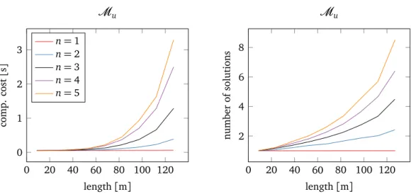
argue that, for indoor spaces, the average complexity is significantly lower and we present a simple algorithm to compute all solutions in a short enough time. We explore computational costs on a real building map in Section 1.4.
Path planning instance We are given: an agent, its navigation line graph L = (NL, EL), n positive cost functions C1≤i≤n(e, x) ∈ R+, source s and a target loca-tions t. We complete L with any edge from s to neighboring cell boundaries, and from all neighbor cell boundaries to t.
The planning problem looks for the best set of paths π ∈ Π on L between source and target according to costs C1≤i≤n. Figure 1.8 illustrates an example of a path given by a sequence of cells and cells boundaries to be crossed when travelling from s to t.
(a) A topological path is computed on the
navigation layer from the lighter to the darker cells. The geometric information about the cells can be used to compute an smooth trajectory (in black), see Chapter 2.
(b) The same path, projected onto other
map layers, provides a rich description. For example, the projection on the smart
cam-era layer informs that the agent will be
par-tially tracked by cameras 3 and 4.
Figure 1.8. A topological pathπ on a multi-layered map.
Optimal solutions In case of a single cost (n = 1), the best possible path is the one that minimizes the total cost in Equation (1.1). We can compute it in polynomial time with respect to the size of L using one of several algorithms for shortest paths on a graph, like Dijkstra’s algorithm.
Instead, when multiple costs need to be minimized, there are multiple sensible ways to define and interpret a solution (see [99] for a complete survey).
Lexicographic order We can define a total ordering between the costs; then,
we choose the path minimizing the first cost; if there are many such paths, we choose the one minimizing the second cost, and so on.
28 1.3 Model
Costs as constraints We could interpret a subset of costs as constraints. That
is, we could define thresholds Cj and imposeCj(π) ≤ Cj for some j’s and
solve for the best path with respect to the remaining costs, using one of the other models presented in this list.
Combination of costs The most intuitive and simplest solution is to combine all
costs in a single cost, for example using a weighted sum.
Pareto front We may define the best set of paths as the Pareto front of the
multi-objective minimization problem, i.e. the set of all non dominated solutions. A dominated solution is a path for which there exists at least another path that is at better (or equal) to it with respect to every cost[20].
In general, to discriminate paths with respect to multiple costs, we need addi-tional criteria that may not be specified at query time. In case of lexical ordering, cost as constraints and combination of costs, the strategic decision is taken be-fore the path is computed by setting the order, the thresholds or the function to combine the costs respectively. On the contrary, the selection of one solution from the Pareto front is delegated (as an informed strategic decision) to the agent afterwards.
In the remaining of this chapter, we consider the multi-objective path plan-ning problem associated with the computation of the Pareto front.
Computation of the Pareto front.
Yen’s algorithm [156] computes iteratively the k-th shortest simple path on a graph and provides the key component to compute the set of optimal paths with respect to a set of costs, as illustrated by Algorithm 4.
The algorithm computes the Pareto front by iteratively applying Yen’s algo-rithm (with respect to switching costs) and adding any non dominated solution until one solution π has been computed by Yen’s algorithm with respect to all costs. In fact, any further application of Yen’s algorithm would compute a path with higher costs than π. Figure 1.9 illustrates this search in cost space in the case of n= 2.
Complexity analysis The time complexity of Yen’s algorithm depends on the
shortest path algorithm that it uses. For example, for using Dijkstra’s algorithm with Fibonacci heap, k applications of Yen’s algorithm have a worst-case time complexity O(k|NL|(|EL| + log |NL|)), which implies a worst-case time complexity
29 1.3 Model 0 2 4 6 8 10 C1 0 2 4 6 8 10 C2
Pareto front search
Figure 1.9. An illustrative example of the computation of the Pareto front Π by Algorithm 4. Each point represents the cost(C1,C2) of a solution in the two di-mensional cost space. The best solution with respect to cost C1(left most point) is computed first; then the best solution with respect to cost C2 (bottom most point), and so on. We keep adding solutions (black dots) to the setΠ, provided they are not dominated by one of the current members of Π (which is not the case for the red solution), following blue or green arrows, which correspond to the computation of the next shortest path using Yen’s algorithm with respect to C1 and C2 respectively. We stop as soon as we find a solution (orange) that has been visited by arrows of all colors. The search is terminated before most gray solutions (which are all dominated) are even computed.
30 1.3 Model
OptimalSolutions(G, s, t,C1, . . . ,Cn)
Π ← ;
forall i∈ {1, . . . , n} do
/* Initialize n instances of Yen’s algorithm */ nextShortestPathi ← Initialize Yen’s generator of shortest paths
between s and t on G with respect to costCi
end i ← 1 do π ←nextShortestPathi() ifπ ∈ Π then addπ to Πi end else
if notdominated(π, Πi,C1, . . . ,Cn) then
addπ to Π addπ to Πi
end end
i← i + 1 mod n
whileπ /∈ Πi for some i∈ {1, . . . , n}
returnΠ dominated(π, Π, C1, . . . ,Cn) forallπ0∈ Π do ifCi(π0) < Ci(π) ∀i = 1, . . . , n then return true end end return false
Algorithm 4: Construction of the Pareto front of all paths between s and t on
31 1.4 Experiments
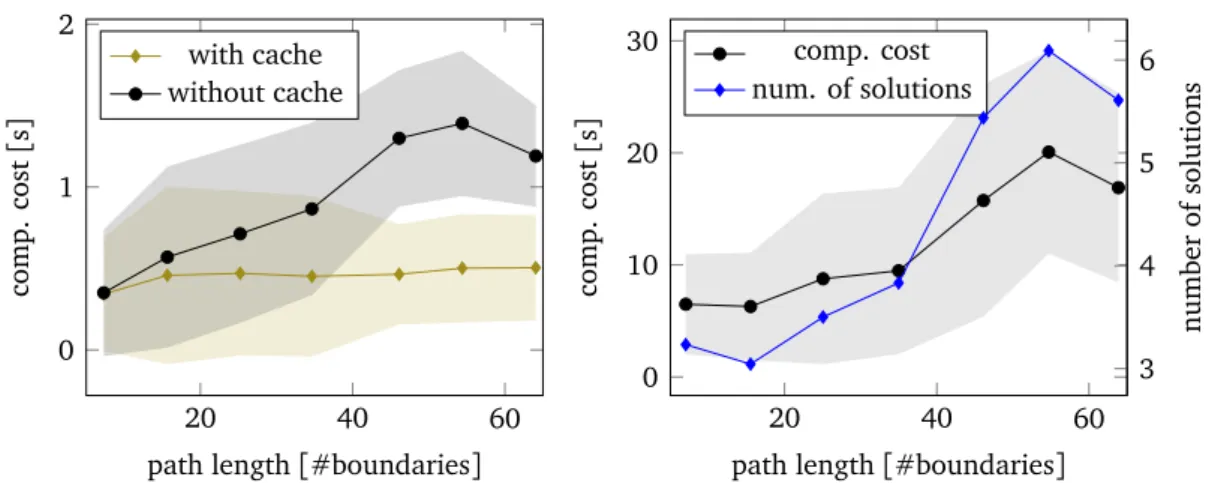
of iterations that the algorithm needs to visit the whole Pareto front. In the worst case, the Pareto front may contain all simple paths from s to t, but in typical indoor maps and cost distributions, the size is usually very limited (see Section 1.4).
Approximations If an approximation of the Pareto front is sufficient, we can
keep the query time limited by stopping Algorithm 4 after a maximal number of iterations. We may also prefer to compute solutions with significantly different costs to reduce the number of strategic choices. In this case, we relax the criteria on dominance to avoid adding almost-dominated solutions [42] in Algorithm 4.
1.4
Experiments
1.4.1
Experimental setup
We test the influence of the number of costs and their spatial distribution on the multi-objective path planning problem formalized in Section 1.3.7 and solved by Algorithm 4. We limit our analysis to a single map but we produce many different planning instances by randomly selecting source, target and cell costs.
Graph We use the (connected) navigation line graph L = (NL, EL) depicted in Figure 1.10 that was automatically derived using Algorithm 2 from the floor map of our building, which has a size of about 120 m×70 m; |NL| = 1638, |EL| = 2310.
Figure 1.10. Map and navigation line graph used to test the impact of the number and the spatial distribution of costs on the planning problem.