DOI 10.1007/s00421-014-2920-z OrIgInAl ArtIclE
A new interpolation‑free procedure for breath‑by‑breath analysis
of oxygen uptake in exercise transients
Aurélien Bringard · Alessandra Adami · Christian Moia · Guido Ferretti
received: 21 november 2013 / Accepted: 21 May 2014 / Published online: 12 June 2014 © Springer-Verlag Berlin Heidelberg 2014
none, unlike Step and linear, indicating that none repro-duced Exact Parameters. noise addition rerepro-duced differ-ences among pre-treatment procedures. Experimental data provided lower phase I time constants with none than with Step.
Conclusion In conclusion, none revealed better precision
and accuracy than Step and linear, especially when phe-nomena characterized by time constants of <30 s are to be analysed. therefore, we endorse the utilization of none to
improve the quality of breath-by-breath ˙VO2 data during
exercise transients, especially when a double exponential model is applied and phase I is accounted for.
Keywords gas exchange · Humans · Kinetics · Procedure Abbreviations
a1 Amplitude of response of first exponential
a2 Amplitude of response of second exponential
b Baseline resting ˙VO2 value
d1 time delay of first exponential
d2 time delay of second exponential
T time
s Second
˙
VO2 Oxygen uptake
θ Heaviside function
τ1 time constant of first exponential
τ2 time constant of second exponential
∈ Mathematical symbol meaning “is an element of”
Introduction
technical developments in the study of the pulmonary gas exchange dynamics at the onset of exercise were character-ized by the attempts at getting rid of two problems, namely:
Abstract
Introduction Interpolation methods circumvent poor
time resolution of breath-by-breath oxygen uptake ( ˙VO2)
kinetics at exercise onset. We report an interpolation-free approach to the improvement of poor time resolution in the analysis of ˙VO2 kinetics.
Methods noiseless and noisy (10 % gaussian noise)
syn-thetic data were generated by Monte carlo method from pre-selected parameters (Exact Parameters). Each data set comprised 10 ( ˙VO2)-on transitions with noisy breath
dis-tribution within a physiological range. transitions were superposed (no interpolation, none), then analysed by bi-exponential model. Fitted model parameters were com-pared with those from interpolation methods (average transition after linear or Step 1-s interpolations), applied on the same data. Experimental data during cycling were also analysed. the 95 % confidence interval around a line of parameters’ equality was computed to analyse agreement between exact parameters and corresponding parameters of fitted functions.
Results the line of parameters’ equality stayed within
confidence intervals for noiseless synthetic parameters with
communicated by carsten lundby.
Electronic supplementary material the online version of this
article (doi:10.1007/s00421-014-2920-z) contains supplementary material, which is available to authorized users.
A. Bringard (*) · A. Adami · c. Moia · g. Ferretti Département de neuroscience Fondamentales, Université de genève, 1 rue Michel Servet, 1211 geneve 4, Switzerland e-mail: [email protected]
g. Ferretti
Dipartimento di Scienze cliniche e Sperimentali, Università di Brescia, Viale Europa 11, 25123 Brescia, Italy
(1) the low time resolution and, (2) the poor signal-to-noise ratio. the most significant advancements in the latter were achieved through the progressive improvement of compu-tational algorithms for the determination of alveolar gas transfer on a breath-by-breath basis.
the first breath-by-breath algorithm was proposed by Auchincloss et al. (1966), who used fixed pre-defined values of functional residual capacity as end-expiratory lung vol-umes in their estimate of the changes in lung gas stores over each breath. Subsequently, several authors introduced vari-ants to the Auchincloss algorithm (Busso and robbins 1997; Swanson and Sherrill 1983; Wessel et al. 1979), to better assess end-expiratory lung volumes. However, di Prampero
and lafortuna (1989) demonstrated that, as long as
end-expiratory lung volume cannot be measured for each single breath, it is not possible to establish the extent to which the alveolar gas exchange variability depends on physiological phenomena using Auchincloss-like algorithms. Other tracks were to be taken. On one side, cala et al. (1996) tried to use external devices. On the other side, capelli et al. (2001)
resumed an alternative algorithm (grønlund 1984), which
got rid of the need of estimating end-expiratory lung vol-ume. With this algorithm, they doubled the signal-to-noise ratio in breath-by-breath determination of alveolar gas transfer as compared with Auchincloss-like algorithms.
Algorithm improvements, however, did not act on the time resolution, although this is a fundamental aspect in the study of gas exchange dynamics. In fact, an abrupt increase
in ventilation and oxygen uptake ( ˙VO2) at the mouth was
frequently observed at exercise start. Some authors attrib-uted this increase to a sudden increase in pulmonary blood
flow (cummin et al. 1986; Wasserman et al. 1974;
Weiss-man et al. 1982). On these bases, Barstow and Molé (1987)
formalized the dynamics of ˙VO2 at exercise start with a
double exponential model. However, the time constant (τ1)
of the first exponential (phase I) turned out to be so low (so fast), that it was systematically undersampled because it was resolved within one, at most two breaths, from exercise start. If a double exponential model of the kinetics of ˙VO2
upon exercise onset is accepted, as is usually the case now-adays, then a correct and precise determination of τ1 and of
the amplitude of phase I (a1) becomes crucial. to this aim,
an improvement of the time resolution in gas exchange analysis is a need. Previous authors tried to increase the time resolution by means of interpolation methods on the 1-s basis (Beaver et al. 1981; Hughson et al. 1993; lamarra et al. 1987), yet introducing distortion of the physiological signal. For this reason, lamarra et al. (1987) suggested that their procedure was to be applied only for analysing phe-nomena with a time constant of at least 30 s.
the aim of this study was to present, evaluate and test a different, new approach to the problem of poor time reso-lution in the analysis of breath-by-breath ˙VO2 kinetics at
exercise onset. With the proposed procedure, possible sig-nal distortion was prevented using superposition of raw
data obtained during several identical ˙VO2-on transients
instead of interpolation, on the assumption that each rep-etition on a given subject is representative of the same
physiological situation. Murgatroyd et al. (2011) already
used superposition of several repetitions together, without interpolation, yet they then averaged the data by n breaths, where n is the total number of repetitions performed, with-out improving time resolution.
Synthetic data generated by Monte carlo simulation procedures were used without and with added noise. Exper-imental data collected during moderate intensity exercise on a cycle ergometer were also obtained. the results were compared with those provided by previous methods of interpolation, applied on the same data sets.
Methods
Synthetic ˙VO2 data generation
A set of synthetic data was generated using the following
bi-exponential model (Barstow and Molé 1987; cautero
et al. 2002; Hughson et al. 1993; lador et al. 2006):
where t is time. the parameter b (in l min−1)
repre-sents the oxygen consumption at rest. the parameters a1
and a2 (both in l min−1) are the amplitudes of the first
and second exponential, respectively, and the param-eters τ1 and τ2 (both in s) the corresponding time
con-stants. the times d1 and d2 are the time delays for the two exponentials. the function θ is the Heaviside function
(θ (t) = 0 if t < 0 and θ (t) = 1 if t ≥ 0).
By means of Eq. (1), 1,000 noiseless sets of ˙VO2 data
had to be generated by Monte carlo method, to encompass the non-uniform gaussian distributions on the following intervals: b ∈ [0.1, 0.6] L min−1, a
1∈ [0.2, 0.8] L min−1,
a2∈ [0.3, 1] L min−1, τ1∈ [0.1, 5] s, τ2∈ [5, 45] s,
d2∈ [8, 35] s and with d1 = 0 s. the amplitudes, time
con-stants and time delays of the 1,000 data sets were defined as Exact Parameters, which were used as reference to define the precision of simulation and experimental results. Experimental ˙VO2 data generation
Eight healthy non-smoking male subjects (age 30.1 ± 5.5 years, height 181 ± 7 cm, body mass
(1) ˙ VO2= b + a1θ (t − d1) 1 − e− t−d1 T1 + a2θ (t − d2) 1 − e− t−d2 T2
73.9 ± 11.4 kg) took part in the experiments. Only subjects with maximal aerobic power equal or higher than 225 W were included. this ensured that the intensity of 80 W that was selected for further experimental tests was in the moder-ate, fully aerobic exercise domain, so that a metabolic steady state was always attained and the τ2 was neither affected by
“early” lactate accumulation (di Prampero and Ferretti 1999) nor influenced by the appearance of the slow component of the ˙VO2 kinetics (Whipp and Wasserman 1972). All subjects
were preliminarily informed of all procedures and risks asso-ciated with the experimental testing. Informed consent was obtained from each volunteer, who was aware of his right of withdrawing from the study at any time without jeopardy. the study was conducted in accordance with the Declaration of Helsinki and was approved by local ethical committee.
the experimental protocol consisted of 10 repetitions of 5-min cycling at 80 W on an electrically braked cycle ergometer (Ergo-metrics 800S, Ergo-line, Blitz, germany). Successive trials were separated by 5 min of recovery at rest. the first repetition of 5-min exercise was preceded by 2 min of rest. the pedalling frequency was kept in the 60–90 rpm range. Each subject, aided by visual feedback, was asked to keep his own pedalling frequency as invariant as possible within each trial and across the 10 trials.
respiratory gas traces and ventilation were continuously measured at the mouth, using a metabolic portable unit
(K4b2, cosmed, rome, Italy), consisting of a zirconium
oxygen analyser, an infrared cO2 metre and a turbine flow-meter. the gas analysers were calibrated with ambient air
and with a gas mixture of known composition (O2 16 %,
cO2 5 %, n2 as balance), and the turbine by means of a 3-l
syringe. Breath-by-breath ˙VO2 and carbon dioxide output
were then computed off-line by means of a modified ver-sion of the grønlund’s algorithm (capelli et al. 2001;
grøn-lund 1984). A software purposely written under the
lab-view® developing environment (labview® 5.0, national
Instruments, Austin, tX, USA) was used.
the none, linear and Step procedures were applied also to the treatment of the 10 repetitions of the experi-mental data sets. However, since the use of 10 repetitions is unlikely in actual experimental conditions, where 3 repeti-tions are performed in most cases, the three pre-treatment procedures were applied to experimental data also using the first 3 repetitions only instead of the entire set of 10 repetitions. So, for each pre-treatment procedure, we had 9 curves of experimental data (one per subject) resulting from 10 repetitions, and 9 curves resulting from the use of the first 3 of these 10 repetitions.
Accounting for irregular time distribution in synthetic data Once the Exact Parameters had been combined to define the synthetic data set, we accounted for the fact that, in a
real experiment, t is not uniformly sampled. In fact t iden-tifies the instant of the actual occurrence of each breath, whose time distribution is irregular and varies with exer-cise time (the breathing frequency increases) and among experiments. to account for this phenomenon, for each of the 1,000 data sets, 10 repetitions were generated. these had the same Exact Parameters, and differed among them only for the time at which each breath occurred. Breath duration in the Monte carlo simulations was let to vary randomly within minima and maxima that were calculated from experimental data. these minima and maxima were defined for each 20-s time window, beginning from exer-cise start. this implied longer breath duration at exerexer-cise start, and progressively shorter breath duration towards the steady state, since minima and maxima tended to decrease moving from one time window to the successive. the 10 repetitions for each data set were generated on an exercise time basis of 5 min, as in actual experimental data acquisi-tion. to give an idea of the degree of breathing frequency variation, we note that breathing frequency of experimental data increased from 16.1 ± 3.9 breaths per minute at rest to 19.4 ± 4.7 breaths per minute at exercise steady state.
these 10 repetitions are noiseless repetitions, in which only t sampling was let to vary. these were subsequently
used to calculate noiseless estimated parameters by “
Fit-ting procedure” (see below). Actual breathing, however, is
affected by noise. to account for the effects of noise, we reanalysed the 10 repetitions, with the same t sampling, after having added also gaussian noise to the synthetic data. the noise added in the present study had a constant standard deviation of 10 %. this value was derived from the statistical analysis of noise performed by lamarra et al. (1987), showing that noise (1) was independent of the work rate, (2) had a typical amplitude for a single transition of ≈10 %, and (3) this amplitude remained unchanged during the entire exercise transient. this second set of data, after addition of noise, was then used to calculate noisy esti-mated parameters by “Fitting procedure” (see below). Data pre-treatment
three pre-treatment procedures were applied on the 10 rep-etitions of the 1,000 data sets for the analysis of the ˙VO2
kinetics. the first procedure, called none, which is the new procedure proposed in this study, requires that the data be used as they came out from the simulation or the actual experiment. thus, no real pre-treatment was performed, apart from pooling all the breaths from the 10 repetitions together on the same plot for further fitting. As a conse-quence, none should merely reconstruct the data curve characterized by the Exact Parameters.
the second procedure, called linear, consisted of a linear interpolation performed between two consecutive
breaths on the data of each of the 10 repetitions. Mean ˙VO2
values were re-computed at 1-s intervals along the interpo-lation line (Barstow and Molé 1991; Hughson et al. 1993), which reconstructed an apparent segmental linearized slope of the ˙VO2 kinetics.
the third procedure, called Step, consisted of a flat interpolation performed on the data of each of the 10 repe-titions, with a 1-s sampling, until the next breath started, at
which time a step increase in ˙VO2 was admitted (lamarra
et al. 1987; Whipp et al. 1982). this procedure is based
on the assumption that the mass flow rates of cO2 and O2
are relatively constant across each breath (cumming 1981;
lamarra et al. 1987).
For linear and Step, within each trial, the interpolated ˙
VO2 value obtained at the end of each second was retained.
then, the 10 pre-treated trials were averaged and the mean ˙
VO2 at each second was computed, thus obtaining the
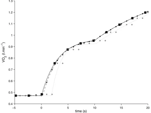
average file on which the fitting procedure was applied. Figure 1 is a schematic representation of the interpolation procedures applied with linear and Step.
the none, linear and Step procedures were applied to the treatment of both noiseless (no noise, but with irregular
t sampling distribution) and noisy (presence of both noise
and irregular t sampling distribution) synthetic data sets. Fitting procedure
the curves obtained by superposing data from 10 repeti-tions (none) and the average curves generated after
appli-cation of linear and Step, provided 1,000 ˙VO2 versus
t series of noiseless or noisy synthetic data, and 8 ˙VO2
versus t series of experimental data, for each
pre-treat-ment procedure. Moreover, we had 8 ˙VO2 versus t series
of experimental data with 3 repetitions instead of 10. the
t at which each breath occurred was defined as the time
when an inspiration began. this was identified as the time when the flow attains zero between an exhalation and the subsequent inspiration. these series were fitted using a non-linear least squares procedure (levenberg–Marquardt
algorithm, see lavenberg 1944; Marquardt 1963, and
−5 0 5 10 15 20 0.4 0.5 0.6 0.7 0.8 0.9 1 1.1 1.2 1.3 time (s) VO 2 (l.min −1)
Fig. 1 Schematic representation of the two interpolation
meth-ods utilized for data pre-treatment. For the sake of clarity the last 5 s of rest, the entire phase I and only the initial seconds of phase II are represented. the filled squares represent the raw points of one repetition of synthetic data. the filled dots refer to the 1-s lin-ear interpolation between consecutive breaths (linlin-ear). the open
dots refer to the 1-s flat interpolation between consecutive breaths with sudden step increase at the next breath (Step). the lines rep-resent the fitted bi-exponential model: continuous line for none,
dashed line for linear and dotted line for Step. the exact
parame-ters were: b = 0.472 l min−1; a
1 = 0.5 l min−1, a2 = 0.6 l min−1,
τ1 = 3 s, τ2 = 23 s, d2 = 10 s and d1 = 0 s. the estimated
param-eters with none were b = 0.472 l min−1; a
1 = 0.500 l min−1,
a2 = 0.600 l min−1, τ1 = 3.000 s, τ2 = 23.000 s, d2 = 10.000 s
and d1 = 0.000 s. the estimated parameters with linear were
b = 0.472 l min−1; a
1 = 0.496 l min−1, a2 = 0.604 l min−1,
τ1 = 2.870 s, τ2 = 22.897 s, d2 = 9.875 s and d1 = 0.242 s.
the estimated parameters with Step were b = 0.472 l min−1;
a1 = 0.458 l min−1, a2 = 0.642 l min−1, τ1 = 1.645 s, τ2 = 21.257 s, d2 = 10.277 s and d1 = 1.893 s
trust-region-reflective algorithm, see coleman and li 1996) with constraints. Equation (1) was used as the fitting model. In other words, the estimated model parameters b, a1, a2, τ1, τ2, d1 and d2 were obtained by minimizing the squared
difference between the model function and the synthetic or experimental ˙VO2 data. constraints were set as follows: (1)
parameters b, a1, a2, τ1, τ2, d1 and d2 could not be negative;
(2) τ2 and d2 were to be larger than τ1 and d1, respectively.
the instant at which exercise started was defined as time 0. the non-linear least square procedure was performed using a function available in the Matlab toolbox (version 7.13.0.564, MathWorks, natick, MA, USA). For syn-thetic data, the starting values were 0.2, 1 l min−1, 5, 30,
0 and 20 s, respectively, for a1, a2, τ1, τ2, d1 and d2.
Start-ing value for b was the individual mean calculated over the last minute of rest before exercise start. For experimental data, the starting values were individually selected based on visual inspection. this carried along the need of testing the robustness of the applied fitting procedure. this was done on synthetic data, by setting different starting values from the Exact Parameters and checking the ensuing output parameters, which turned out independent of the applied starting values.
this fitting procedure was applied to both noiseless and noisy synthetic data sets, to obtain, respectively, noiseless estimated parameters and noisy estimated parameters, as defined above. If pre-treatment procedures were not intro-ducing errors, noiseless estimated parameters would result equal to the Exact Parameters. In this case, if we plot the former as a function of the latter parameters, all points should lie on the line of parameters’ equality. Because of noise, noisy estimated parameters should not lie on the line of parameters’ equality; however, the precision and accuracy of their distribution around the line of param-eters’ equality will be best, the highest is the coincidence between noiseless estimated parameters and Exact Param-eters. the parameters estimated on the experimental data were defined as experimental parameters.
Statistical analysis
For the experimental data, the effects of the pre-treatment procedure and of the number of repetitions on the experi-mental parameters were analysed by two-way analysis of variance for repeated measures. When applicable, a tukey post hoc test was used to locate significant differences. these analyses were performed using commercial statistical software (Statistica version 11, Stat Soft. Inc., tulsa, OK, USA). the results were considered significant if p < 0.05. For each parameter, individual confidence intervals were calculated based on the Jacobian provided by the fitting function, using a function available in the Matlab toolbox (version 7.13.0.564, MathWorks, natick, MA, USA).
For the synthetic data with all pre-treatment
meth-ods, the 95 % confidence intervals were estimated for a1,
a2, d2, τ1 and τ2 by bootstrap, using the bias corrected and
accelerated percentile method using a function available in the Matlab toolbox (version 7.13.0.564, MathWorks, natick, MA, USA), and encompassing the whole range of Exact Parameters used in the Monte carlo simulation (see “Synthetic V˙O2 data generation”). the 95 %
boot-strap confidence interval was computed on 5,000 bootboot-strap samples (random sampling from the original data set with replacement), on which a linear regression was calculated, yielding a total of 5,000 slopes. the input of the function included either the 1,000 noiseless or the 1,000 noisy syn-thetic data. the output was a vector containing the lower and upper bounds of the confidence interval, calculated for the whole range of the Exact Parameters.
the influence of d2 value on the other parameters of
the noiseless synthetic data was estimated by calculating,
for bins of exact d2 values, the percentage of estimated
parameters that are closer than a certain error margin from
the corresponding Exact Parameters. the bins of exact d2
were 8–12, 12–16, 16–20, 20–24, 24–30, 30–35 s, covering all the intervals of d2 values selected for the Monte carlo
method, by which the synthetic ˙VO2 data were generated.
the error margins selected were equivalent to once the width of the confidence intervals for none, as calculated by bootstrap, at the median of the range of exact values for each parameter. At these medians, the retained error mar-gins resulted 0.0717, 0.1208 s, 0.0055 and 0.0054 l min−1,
for τ1, τ2, a1 and a2, respectively, for noiseless estimated
parameters. the corresponding retained error margins for noisy estimated parameters were 0.1387, 0.3215 s, 0.0064 and 0.0061 l min−1, respectively, for τ
1, τ2, a1 and a2.
Results
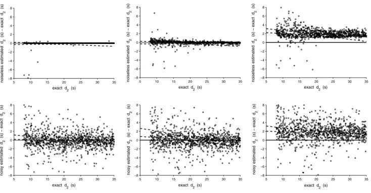
the differences between noiseless estimated d2 values and
the corresponding exact d2 values are shown in the upper
panels of Fig. 2 as a function of exact d2. Whereas none
and linear provided good estimates of d2, Step
overesti-mated d2, as demonstrated by the line of parameters’
equal-ity lying below the lower confidence interval curve. the differences between noisy estimated d2 values and the cor-responding exact d2 values are shown in the lower panels of Fig. 2 as a function of exact d2. Although noisy data were
more scattered than noiseless data for all three methods,
none and linear provided good noisy estimated d2 values,
whereas Step again overestimated d2.
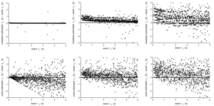
the same type of analyses reported in Fig. 2 for d2 was
performed for estimated τ1, τ2, a1 and a2. the difference
between these estimated parameters and the correspond-ing Exact Parameters were plotted as a function of the
corresponding Exact Parameters. the plots concerning τ1
are shown in Fig. 3, the plots concerning, τ2, a1 and a2 are
presented as Supplementary material. noiseless estimated parameters appear in the upper panels, noisy estimated parameters in the lower panels. As far as none is con-cerned, it is noteworthy that several data still lay outside the confidence intervals. Obviously enough, the fraction of data outside the confidence intervals was greater for noisy than for noiseless estimated parameters. With none the line of parameters’ equality stayed within the confidence inter-vals for all noiseless estimated parameters. these tenden-cies were less evident in the case of noisy estimated param-eters (lower panels of Figs. 2, 3, and of figures provided as Supplementary material), due to wider data dispersion. In this case, the line of parameters’ equality was close to the upper or the lower confidence interval for d2, τ1, τ2, a1, a2.
When also linear and Step were accounted for, in both cases, it appeared that the number of noiseless estimated parameters lying outside the line of parameters’ equality was more numerous than for none. Symmetrically, for all fitting parameters, the fraction of synthetic values lying exactly on the line of parameters’ equality was larger with none than with linear and Step. concerning Step and lin-ear, it is noteworthy that both procedures provided line of parameters’ equality below the lower confidence interval curve for τ1, indicating that they overestimated τ1 (Fig. 3,
upper panels). Moreover, as can be seen in the Figures that we uploaded as Supplementary material, both proce-dures overestimated τ2, and tended to overestimate a1 and
to underestimate a2. Yet concerning noiseless τ2, we remark
a tendency to approach the line of parameter’s equality at high exact τ2 values. All pre-treatment procedures provided
a good estimate of the total ˙VO2 change between rest and
steady state, which is equal to the sum of a1 plus a2.
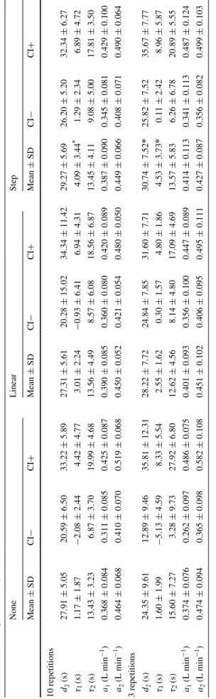
the experimental data are shown in table 1, where the
experimental parameters obtained with the three
pre-treat-ment procedures are reported. With 10 repetitions, τ1 was
significantly shorter with none than with the two other pro-cedures. no differences among pre-treatment procedures were found for phase II parameters. no significant differ-ences between 10 and 3 repetitions were found. neverthe-less, with three repetitions, τ1 with none was significantly
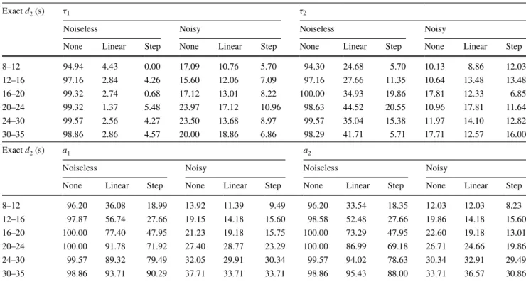
shorter than that with Step, but not than that with linear. the fraction of estimated data that deviated from the Exact Parameters by less than the width of the confidence
intervals was reported in table 2 for each considered
range of exact d2 values, for none, linear and Step. For
τ1, the fraction of noiseless estimated data deviating from
the Exact Parameters by less than once the width of the confidence intervals with linear and Step remained always below 5 %, even with the longest d2 values. For all param-eters, this fraction for none was above 94 % for all the d2
5 10 15 20 25 30 35 −8 −6 −4 −2 0 2 4 6 8 exact d2 (s) noiseless estimated d2 (s) − exact d2 (s) 5 10 15 20 25 30 35 −8 −6 −4 −2 0 2 4 6 8 exact d2 (s) noiseless estimated d2 (s) − exact d2 (s) 5 10 15 20 25 30 35 −8 −6 −4 −2 0 2 4 6 8 exact d2 (s) noiseless estimated d2 (s) − exact d2 (s) 5 10 15 20 25 30 35 −8 −6 −4 −2 0 2 4 6 8 exact d2 (s) noisy estimated d2 (s) − exact d2 (s ) 5 10 15 20 25 30 35 −8 −6 −4 −2 0 2 4 6 8 exact d2 (s) noisy estimated d2 (s) − exact d2 (s ) 5 10 15 20 25 30 35 −8 −6 −4 −2 0 2 4 6 8 exact d2 (s) noisy estimated d2 (s) − exact d2 (s )
Fig. 2 Top the difference between noiseless estimated d2 and exact
d2 is plotted as a function of exact d2. For none (left panel), linear (middle panel) and Step (right panel). the horizontal line is the line of parameter’s equality (y = 0); the dotted lines represent the con-fidence intervals calculated by bootstrap (5,000 resampling). Bottom
the difference between noisy estimated d2 and exact d2 is plotted as a function of exact d2, for none (left panel), linear (middle panel) and Step (right panel). the horizontal line is the line of parameter’s equality (y = 0); the dotted lines represent the confidence intervals calculated by bootstrap (5,000 resampling). N = 1,000
ranges. By contrast, the corresponding fractions of noisy estimated τ1 and τ2 data deviating from the Exact
Param-eters by less than once the width of the confidence intervals was never higher than 24, 19 and 16 %, respectively, for none, linear and Step. A better precision was attained in the estimate of amplitudes than in that of time constants, for all pre-treatment methods.
Discussion
In this study, we presented a new procedure for breath-by-breath analysis of ˙VO2-on kinetics without intra-breath
interpolation treatment (none). the results obtained with none were compared with those obtained by applying on the same data two commonly used pre-treatment proce-dures, both characterized by application of 1-s intra-breath interpolation methods with subsequent computation of
the mean ˙VO2 value at each second over several
repeti-tions of the same test (here defined as Step and linear). this was done on (1) high-quality noise-free synthetic data obtained by means of Monte carlo simulations, (2) the same sets of synthetic data after addition of 10 % gauss-ian noise, and (3) physiological data obtained on exercising humans (experimental data). In the first case, we stressed
the distortion effect of the interpolation procedures with respect to the none method––which on this basis may theoretically be considered a more correct approach––with-out other confounding factors; in the second, we added a dumping effect of signal noise, common to all tested condi-tions, tending to minimize differences among methods; this dumping effect was even enlarged in the third case, where other sources of random noise, actually present in real experimental conditions, were further introduced. As a con-sequence, noiseless synthetic data highlighted the effect of pre-treatment alone, in absence of other confounding fac-tors, thus providing a direct demonstration of the impact of pre-treatment on model parameters. the addition of gauss-ian noise to synthetic data, plus that of random noise com-ing from experimental data, allowed then an evaluation of the tendencies revealed on noiseless data in conditions pro-gressively approaching the “physiological” one.
the three procedures only differed by the pre-treatment, whereas the ˙VO2 computation algorithm and the fitting
pro-cedure were the same. the results of the noiseless synthetic data demonstrated that none was the best approach to the estimate of τ1. In fact, Fig. 3 showed that none provided
the least data shift with respect to the exact data, repre-sented by the line of parameters’ equality. this conclusion can be confirmed after analysis of noisy estimated data and,
0 1 2 3 4 5 −3 −2 −1 0 1 2 3 exact τ1 (s) noiseless estimated τ1 (s) − exact τ1 (s ) 0 1 2 3 4 5 −3 −2 −1 0 1 2 3 exact τ1 (s) noiseless estimated τ1 (s) − exact τ1 (s ) 0 1 2 3 4 5 −3 −2 −1 0 1 2 3 exact τ1 (s) noiseless estimated τ1 (s) − exact τ1 (s ) 0 1 2 3 4 5 −3 −2 −1 0 1 2 3 exact τ1 (s) noisy estimated τ1 (s) − exact τ1 (s ) 0 1 2 3 4 5 −3 −2 −1 0 1 2 3 exact τ1 (s) noisy estimated τ1 (s) − exact τ1 (s ) 0 1 2 3 4 5 −3 −2 −1 0 1 2 3 exact τ1 (s) noisy estimated τ1 (s) − exact τ1 (s )
Fig. 3 Top the difference between noiseless estimated time
con-stant of the first exponential (noiseless estimated τ1), obtained after
application of none (top left panel), linear (top middle panel) and Step (top right panel), and the corresponding exact values (exact τ1
), is reported as a function of the corresponding exact τ1. Each point
(N = 1,000) was obtained using the combined data of the 10 repeti-tions. the horizontal line is the line of parameter’s equality (y = 0);
the dotted lines represent the confidence intervals calculated by boot-strap (5,000 resampling). Bottom the difference between noisy esti-mated τ1 and exact τ1 is plotted as a function of exact τ1, for none (left panel), linear (middle panel) and Step (right panel). the horizontal
line is the line of parameter’s equality (y = 0); the dotted lines
rep-resent the confidence intervals calculated by bootstrap (5,000 resam-pling). N = 1,000
Table
1
Experimental P
arameters as calculated by the model from the e
xperimental data: comparison of results from the three pre-treatment procedures, for the whole set of 10 repetitions (top)
and for the first 3 repetitions only (bottom) Data are gi
ven as mean and standard de
viation (SD), with the a
verage of the lo wer ( c I− ) and upper ( c I+ ) indi vidual 95 % confidence interv als bounds d2
time delay of the second e
xponential,
τ1
time constant of the first e
xponential,
τ2
time constant of the second e
xponential,
a1
amplitude of the first e
xponential,
a2
amplitude of the second
exponential * Significantly dif
ferent from n one. N = 8 n one l inear Step Mean ± SD c I− c I+ Mean ± SD c I− c I+ Mean ± SD c I− c I+ 10 repetitions d 2 (s) 27.91 ± 5.05 20.59 ± 6.50 33.22 ± 5.89 27.31 ± 5.61 20.28 ± 15.02 34.34 ± 11.42 29.27 ± 5.69 26.20 ± 5.20 32.34 ± 6.27 τ1 (s) 1.17 ± 1.87 − 2.08 ± 2.44 4.42 ± 4.77 3.01 ± 2.24 − 0.93 ± 6.41 6.94 ± 4.31 4.09 ± 3.44 * 1.29 ± 2.34 6.89 ± 4.72 τ2 (s) 13.43 ± 3.23 6.87 ± 3.70 19.99 ± 4.68 13.56 ± 4.49 8.57 ± 6.08 18.56 ± 6.87 13.45 ± 4.11 9.08 ± 5.00 17.81 ± 3.50 a1 ( l min − 1) 0.368 ± 0.084 0.311 ± 0.085 0.425 ± 0.087 0.390 ± 0.085 0.360 ± 0.080 0.420 ± 0.089 0.387 ± 0.090 0.345 ± 0.081 0.429 ± 0.100 a2 ( l min − 1) 0.464 ± 0.068 0.410 ± 0.070 0.519 ± 0.068 0.450 ± 0.052 0.421 ± 0.054 0.480 ± 0.050 0.449 ± 0.066 0.408 ± 0.071 0.490 ± 0.064 3 repetitions d 2 (s) 24.35 ± 9.61 12.89 ± 9.46 35.81 ± 12.31 28.22 ± 7.72 24.84 ± 7.85 31.60 ± 7.71 30.74 ± 7.52 * 25.82 ± 7.52 35.67 ± 7.77 τ1 (s) 1.60 ± 1.99 − 5.13 ± 4.59 8.33 ± 5.54 2.55 ± 1.62 0.30 ± 1.57 4.80 ± 1.86 4.53 ± 3.73 * 0.11 ± 2.42 8.96 ± 5.87 τ2 (s) 15.60 ± 7.27 3.28 ± 9.73 27.92 ± 6.80 12.62 ± 4.56 8.14 ± 4.80 17.09 ± 4.69 13.57 ± 5.83 6.26 ± 6.78 20.89 ± 5.55 a1 ( l min − 1) 0.374 ± 0.076 0.262 ± 0.097 0.486 ± 0.075 0.401 ± 0.093 0.356 ± 0.100 0.447 ± 0.089 0.414 ± 0.113 0.341 ± 0.113 0.487 ± 0.124 a2 ( l min − 1) 0.474 ± 0.094 0.365 ± 0.098 0.582 ± 0.108 0.451 ± 0.102 0.406 ± 0.095 0.495 ± 0.111 0.427 ± 0.087 0.356 ± 0.082 0.499 ± 0.103
although at a lesser extent, after analysis of experimental data.
Intuitively, the apparent best performance of none can be explained by the fact that linear and Step distort the recorded data and thus indirectly influence the constants describing the model’s function. In the case of linear and Step, this effect is not completely predictable because we are in presence of non-uniform breath sampling––that is random-like––in the time domain. this means that the influence of the interpolation procedures on two identical ˙
VO2 kinetics repetitions, and thus on the model’s constants,
is not the same in different trials, because the sampling times change at each repetition of the experimental pro-tocol. In other words, the distortive effect depends on the sampling’s characteristics.
Fitting procedures are such that any fitting model, which moves smoothly through the data, is tantamount to a pre-cise filter for the data. Assuming that all repetitions carried out by one given subject, who performs a given exercise with identical protocol, are indeed representative of the same experimental condition, superposing data points from different repetitions of the same well-controlled event, as done with none, provides the necessary amount of data points allowing for a highly accurate computation of model
parameters by the fitting procedure. this is a general con-cept, which holds for any type of experimental condition and model fitting procedure, wherein repeated discrete measurements of the same event in the same condition are made. this being the case, there is no need of introducing
data interpolation procedures in the analysis of ˙VO2-on
kinetics, as done with Step and linear.
the model analysis of the ˙VO2-on kinetics in this study
was carried out using the double exponential model that
Barstow and Molé (1987) developed after an original idea
of Wasserman et al. (1974). the model was widely used
ever since, and was thoroughly criticized by lador et al. (2006), who first applied the same concept to the analysis of beat-by-beat kinetics of cardiac output. We are neverthe-less aware of the incompleteness of this model, which does not account for pulsatile phenomena affecting pulmonary blood flow, as a consequence of the rhythmic activity of the heart and of the lungs and of the heterogeneous recruitment of lung capillaries (Arieli 1983; Marconi et al. 1988; Meyer et al. 1989; West et al. 1964). Further advances in model-ling should account also for these phenomena.
In the context of the double exponential model of
Barstow and Molé (1987), a comparison of the three
pre-treatment methods, carried out on noiseless synthetic data,
Table 2 Percentage of model’s parameters from synthetic data with
estimated errors (difference between noiseless estimated parameters and the corresponding exact parameters and between noisy estimated
parameters and the corresponding exact parameters) that are smaller than the confidence intervals: comparison of results from the three pre-treatment procedures, as a function of exact d2
Data are given as a percentage of the total noiseless estimated and noisy estimated parameters for bins of exact d2, for each pre-treatment proce-dure
d2 time delay of the second exponential, τ1 time constant of the first exponential, τ2 time constant of the second exponential, a1 amplitude of the
first exponential, a2 amplitude of the second exponential
Exact d2 (s) τ1 τ2
noiseless noisy noiseless noisy
none linear Step none linear Step none linear Step none linear Step
8–12 94.94 4.43 0.00 17.09 10.76 5.70 94.30 24.68 5.70 10.13 8.86 12.03 12–16 97.16 2.84 4.26 15.60 12.06 7.09 97.16 27.66 11.35 10.64 13.48 13.48 16–20 99.32 2.74 0.68 17.12 13.01 8.22 100.00 34.93 19.86 17.81 12.33 6.85 20–24 99.32 1.37 5.48 23.97 17.12 10.96 98.63 44.52 20.55 10.96 17.81 11.64 24–30 99.57 2.56 4.27 23.50 13.68 8.97 99.57 35.04 15.38 11.97 14.10 12.82 30–35 98.86 2.86 4.57 20.00 18.86 6.86 98.29 41.71 5.71 17.71 12.57 16.00 Exact d2 (s) a1 a2
noiseless noisy noiseless noisy
none linear Step none linear Step none linear Step none linear Step
8–12 96.20 36.08 18.99 13.92 11.39 9.49 96.20 33.54 18.35 12.03 12.03 8.23 12–16 97.87 56.74 27.66 19.15 14.18 15.60 98.58 52.48 27.66 19.86 14.18 15.60 16–20 100.00 77.40 47.95 21.23 19.18 15.75 100.00 73.29 47.95 22.60 19.18 13.01 20–24 100.00 91.78 71.92 27.40 28.77 23.29 100.00 86.99 69.18 26.71 24.66 19.86 24–30 99.57 89.32 79.49 32.05 29.91 30.34 99.57 94.02 78.63 30.34 32.91 29.49 30–35 98.86 93.71 90.29 37.71 33.71 33.71 98.86 95.43 88.00 33.71 36.57 30.86
showed that none was more precise than linear and Step in describing the ˙VO2-on kinetics, as demonstrated by the
distribution of points on the line of parameters’ equality. Among the parameters estimated by the bi-exponential model, the largest differences between the three pre-treat-ment procedures were observed for τ1 (Fig. 3), as expected.
none showed less point scattering (imprecision) than lin-ear, and particularly than Step. It provided the best estimate of τ1 with respect to the exact values, whereas linear and
Step clearly and systematically overestimated τ1. In other
terms, τ1 resulted smaller (faster) with none than with any
of the two other methods. this is in line with the expec-tations associated with the introduction of interpolation procedures with linear and Step. to sum up, due to the absence of added data interpolation, none can be consid-ered as the best of the three tested procedures when fast temporal parameters, like τ1, are to be estimated.
All three procedures provided more precise results in estimating τ2 than τ1, because τ2 was computed on a greater
number of data points, due to the longer duration of phase II of the ˙VO2 kinetics and to the concomitant increase in
breathing frequency. In spite of this, the analysis of both noiseless and noisy synthetic data shows that linear and
Step still overestimated τ2, especially when it was low,
but this tendency was progressively reduced as long as τ2
was increased, to disappear for τ2 values higher than 35 s.
this is coherent with the concept that the distortive effect of Step and linear on calculated parameters was inevitably less, the higher was τ2. this effect was not such as to affect
experimental τ2 values, which were similar, and did not
dif-fer significantly among the three pre-treatment procedures.
the low experimental τ2 values are therefore not a
conse-quence of none with respect to Step and linear. they may rather be an intrinsic consequence of the grønlund
algo-rithm, as demonstrated by cautero et al. (2003), combined
with the lightness of the selected power, well below the ventilatory threshold in all subjects. At comparable pow-ers, similar results to the present ones (τ2 of 14.1 ± 6.6 s,
Aliverti et al. 2009) were obtained using a direct estimate of end-expiratory lung volumes with an opto-electronic plethysmography technique (cala et al. 1996).
concerning amplitudes, tendencies to overestimate a1 by
linear and Step were counteracted by opposite tendencies to underestimate a2. As a consequence, the total amplitude of the ˙VO2 response (a1 + a2) was fairly well estimated by
all pre-treatment procedures, in agreement with the notion that they all are sufficiently accurate when used in steady state conditions, because the “flatness” of the breath time series underscores the distortive effect of the interpolation method.
the presence of noise reduced in all cases the method’s precision, as shown by the increase in data dispersion around the line of parameters’ equality and by the smaller
fraction of data within one confidence interval for noisy synthetic data than for noiseless synthetic data (table 2). this, however, did not affect accuracy, as long as in Fig. 3 and in Supplementary material, the line of parameters’ equality remained outside the confidence intervals for lin-ear and Step, contrary to none. to sum up, when noise-less synthetic data are accounted for, none resulted both very precise and accurate, because there was no noise and no data distortion, whereas linear and Step were less pre-cise than none, despite the absence of noise, and inaccu-rate, due to data distortion. When noisy synthetic data are accounted for instead, there was in all cases a loss of preci-sion due to the introduction of noise, but since noise did not affect accuracy, none remained accurate and linear and Step remained inaccurate.
lamarra et al. (1987), who first proposed and discussed Step, were aware of the fact that Step introduces a filter whose time constant is the mean breath duration, which removes only high-frequency fluctuations. coherently, we demonstrated on noiseless synthetic data that the accuracy
of Step tended to increase with increasing τ2. Although
Step provided a correct estimate of τ2 when this was higher
than 35 s, it must not be used when time constants lower than 30 s are expected.
linear (Barstow and Molé 1991; Hughson et al. 1993)
tried to circumvent the limits of Step through an appar-ently less distortive interpolation. the noisy synthetic data reported in table 2 indicated that it succeeded at least
partly, since for a large number of d2 ranges linear
pro-vided better performance than Step, especially as far as the
computation of τ1 was concerned. the physiological
con-cept behind linear is that the rate of alveolar gas exchange varies within a single breath, so that we may assume a continuous ˙VO2 increase from one breath to the next
dur-ing the ˙VO2-on kinetics. this ˙VO2 increase was considered
to be linear. Yet the distortive effect was still maintained,
especially in the determination of τ1, whose values may
be within the duration of a single breath. In fact linear still remained an inaccurate method, as demonstrated by its overestimate of τ1, and by no means had it attained the
accuracy and precision of none (Fig. 3).
coherently with the synthetic data, experimental data showed the same amplitudes for the three pre-treatment methods. Significant differences were observed only for τ1,
as none provided, as expected, faster (lower) values than Step. As discussed above, this may be due to the filter-like effect implicit in the latter procedures. the 2-s difference for d2 with Step, although non-significant, corresponds to the shift with respect to the line of parameters’ equality observed for Step on noisy data (Fig. 2, lower right panel).
When 3 repetitions were considered instead of 10, the lack of significant differences with respect to the lat-ter suggested that 3 repetitions may be enough indeed for
a satisfactory analysis of the ˙VO2-on kinetics. A closer
inspection of the data, however, revealed some ambiguities. With three repetitions in fact (1) d2 turned out significantly lower with none than with Step; (2) τ2 tended to be slower
with none. Despite the suggestions of this study, a more specific study, aimed at identifying more accurately the minimum number of repetitions for the establishment of a correct ˙VO2-on kinetics should be envisaged.
In this study, we did not consider d2 values lower
than 8 s, because d2 represents the blood transit time from
contracting muscles to lungs at exercise start, which is between 7 and 9 s at the present steady state metabolic rate
(Barstow and Molé 1987; lindholm et al. 2006; Whipp
et al. 1982). In fact table 2 shows that for none there was no effect of d2 on the fraction of synthetic noiseless data that deviated from the Exact Parameters by less than the width of the confidence intervals. By contrast, this was not so with linear and Step, for which the lower were the exact d2 values, the less precise were the corresponding estimated τ2, a1 and a2.
Conclusions
In conclusion, none revealed better precision and accuracy than Step and linear, especially when phenomena char-acterized by time constants of <30 s are to be analysed. the addition of noise, however, reduced the differences among pre-treatment procedures, so that none maintained an added value with respect to linear only for the com-putation of time constants, but not for the comcom-putation of amplitudes. therefore, we endorse the utilization of none as a tool to improve the quality of breath-by-breath pul-monary gas exchange analysis during exercise transients, especially when a double exponential model (Barstow and Molé 1987) is applied and phase I is accounted for. We are nevertheless aware that, although these results represent a significant step forward in the treatment of experimental breath-by-breath data under unsteady state conditions, fur-ther computational developments, accounting also for the effects of concomitant oscillatory mechanisms, are still necessary to attain a fully satisfactory comprehension of the breath-by-breath ˙VO2 data.
Acknowledgments this study was supported by Swiss national
Science Foundation grants 32003B_127620 and 32003B_143427 to guido Ferretti. the authors thank the volunteers for their implication in this study.
References
Aliverti A, Kayser B, cautero M, Dellacà rl, di Prampero PE, capelli c (2009) Pulmonary V̇O2 kinetics at the onset of exercise
is faster when actual changes in alveolar O2 stores are considered. respir Physiol neurobiol 169:78–82
Arieli r (1983) cardiogenic oscillations in expired gas: origin and mechanism. respir Physiol 52:191–204
Auchincloss JH Jr, gilbert r, Baule gH (1966) Effect of ventila-tion on oxygen transfer during early exercise. J Appl Physiol 21:810–818
Barstow tJ, Molé PA (1987) Simulation of pulmonary O2 uptake dur-ing exercise transients in humans. J Appl Physiol 63:2253–2261 Barstow tJ, Molé PA (1991) linear and nonlinear characteristics of
oxygen uptake kinetics during heavy exercise. J Appl Physiol 71:2099–2106
Beaver Wl, lamarra n, Wasserman K (1981) Breath-by-breath measurement of true alveolar gas exchange. J Appl Physiol 51:1662–1675
Busso t, robbins PA (1997) Evaluation of estimates of alveolar gas exchange by using a tidally ventilated nonhomogenous lung model. J Appl Physiol 82:1963–1971
cala SJ, Kenyon cM, Ferrigno g, carnevali P, Aliverti A, Pedotti A, Macklem Pt, rochester DF (1996) chest wall and lung volume estimation by optical reflectance motion analysis. J Appl Physiol 81:2680–2689
capelli c, cautero M, di Prampero PE (2001) new perspectives in breath-by-breath determination of alveolar gas exchange in humans. Pflugers Arch 441:566–577
cautero M, Beltrami AP, di Prampero PE, capelli c (2002) Breath-by-breath alveolar oxygen transfer at the onset of step exercise in humans: methodological implications. Eur J Appl Physiol 88:203–213
cautero M, di Prampero PE, capelli c (2003) new acquisitions in the assessment of breath-by-breath alveolar gas transfer in humans. Eur J Appl Physiol 90:231–241
coleman tF, li Y (1996) An interior, trust region approach for nonlinear minimization subject to bounds. SIAM J Optim 6:418–445
cummin Ar, Iyawe VI, Mehta n, Saunders KB (1986) Ventilation and cardiac output during the onset of exercise, and during volun-tary hyperventilation, in humans. J Physiol 370:567–583 cumming g (1981) gas mixing in disease. In: Scadding JD,
cum-ming g (eds) Scientific foundations of respiratory medicine. Heinemann, london, pp 688–697
di Prampero PE, Ferretti g (1999) the energetics of anaerobic mus-cle metabolism: a reappraisal of older and recent concepts. respir Physiol 118:103–115
di Prampero PE, lafortuna cl (1989) Breath-by-breath estimate of alveolar gas transfer variability in man at rest and during exer-cise. J Physiol 415:459–475
grønlund J (1984) A new method for breath-to-breath determination of oxygen flux across the alveolar membrane. Eur J Appl Physiol Occup Physiol 52:167–172
Hughson rl, cochrane JE, Butler gc (1993) Faster O2 uptake kinet-ics at onset of supine exercise with than without lower body neg-ative pressure. J Appl Physiol 75:1962–1967
lador F, Azabji Kenfack M, Moia c, cautero M, Morel Dr, capelli c, Ferretti g (2006) Simultaneous determination of the kinetics of cardiac output, systemic O2 delivery, and lung O2 uptake at exercise onset in men. Am J Physiol regul Integr comp Physiol 290:r1071–r1079
lamarra n, Whipp BJ, Ward SA, Wasserman K (1987) Effect of inter-breath fluctuations on characterizing exercise gas exchange kinet-ics. J Appl Physiol 62:2003–2012
lavenberg K (1944) A method for the solution of certain problems in least squares. Quart Appl Math 2:164–168
lindholm D, Karlsson l, gill H, Wigertz O, linnarsson D (2006) time components of circulatory transport from the lungs to a peripheral artery in humans. Eur J Appl Physiol 97:96–102
Marconi c, Heisler n, Meyer M, Weitz H, Pendergast Dr, cerretelli P, Piiper J (1988) Blood flow distribution and its temporal vari-ability in stimulated dog gastrocnemius muscle. respir Physiol 74:1–13
Marquardt D (1963) An algorithm for least-squares estimation of non-linear parameters. SIAM J Appl Math 11:431–441
Meyer M, calzia E, Mohr M, Schulz H, neufeld g, Piiper J (1989) cardiogenic mixing: mechanisms and experimental evidence in dogs. Br J Anaesth 63(Suppl 1):95S–101S
Murgatroyd Sr, Ferguson c, Ward SA, Whipp BJ, rossiter HB (2011) Pulmonary O2 uptake kinetics as a determinant of high-intensity exercise tolerance in humans. J Appl Physiol 110(6):1598–1606 Swanson gD, Sherrill Dl (1983) A model evaluation of estimates
of breath-to-breath alveolar gas exchange. J Appl Physiol 55:1936–1941
Wasserman K, Whipp BJ, castagna J (1974) cardiodynamic hyper-pnea: hyperpnea secondary to cardiac output increase. J Appl Physiol 36:457–464
Weissman Ml, Jones PW, Oren A, lamarra n, Whipp BJ, Wasser-man K (1982) cardiac output increase and gas exchange at start of exercise. J Appl Physiol 52:236–244
Wessel HU, Stout rl, Bastanier cK, Paul MH (1979) Breath-by-breath variation of Frc: effect on VO2 and VcO2 measured at the mouth. J Appl Physiol 46:1122–1126
West JB, Dollery ct, naimark A (1964) Distribution of blood flow in isolated lung; relation to vascular and alveolar pressures. J Appl Physiol 19:713–724
Whipp BJ, Wasserman K (1972) Oxygen uptake kinetics for various intensities of constant-load work. J Appl Physiol 33:351–356 Whipp BJ, Ward SA, lamarra n, Davis JA, Wasserman K (1982)
Parameters of ventilatory and gas exchange dynamics during exercise. J Appl Physiol 52:1506–1513