Risk Appetite in Practice: Vulgaris Mathematica

HAL Id: halshs-01020293

https://halshs.archives-ouvertes.fr/halshs-01020293

Submitted on 8 Jul 2014

HAL is a multi-disciplinary open access

archive for the deposit and dissemination of sci-entific research documents, whether they are pub-lished or not. The documents may come from

L’archive ouverte pluridisciplinaire HAL, est destinée au dépôt et à la diffusion de documents scientifiques de niveau recherche, publiés ou non, émanant des établissements d’enseignement et de

Risk Appetite in Practice: Vulgaris Mathematica

Bertrand K. Hassani

To cite this version:

Documents de Travail du

Centre d’Economie de la Sorbonne

Risk Appetite in Practice: Vulgaris Mathematica

Bertrand K. H

Risk Appetite in Practice: Vulgaris Mathematica

April 14, 2014

Author

• Bertrand K. Hassani1: Santander UK and Université Paris 1 Panthéon-Sorbonne CES UMR

8174, 2 Triton Square, NW1 3AN London, United Kingdom, phone: +44 (0)7530167299, e-mail: bertrand.hassani@santander.co.uk

Abstract

The ultimate goal of risk management is the generation of efficient incomes. The objec-tive is to generate the maximum return for a unit of risk taken or to minimise the risk taken to generate the return expected i.e. it is the optimisation of a financial institution strategy. Therefore, by measuring its exposure against its appetite, a financial institution is assessing its couple risk-return. But this task may be difficult as banks face various types of risks, for instance, Operational, Market, Credit, Liquidity, etc. and these cannot be evaluated on a stand alone basis, interaction and contagion effects should be taken into account. In this paper, methodologies to evaluate banks’ exposures are presented along their management implications, as the purpose of the risk appetite evaluation process is the transformation of risk metrics into effective management decisions.

Keywords: Risk Management - Risk Measures - Risk Appetite - Interdependencies

1

Disclaimer: The opinions, ideas and approaches expressed or presented are those of the authors and do not necessarily reflect Santander’s position. As a result, Santander cannot be held responsible for them.

1

Introduction

Paraphrasing Warren Buffet, “Risks arise by not knowing what you are doing”, the recent events and the popular prosecusion led governments, authorities and regulator to ask the following ques-tions: do the financial institutions understand the risks they are taking? Is this one properly measured? Regulatory requirements arose (FSB (2013), BCBS (2013)) demanding bank to as-sess their risk appetite in order to answer these questions. However, the discussion around the terminologies and there implications are still on going, as for example it is complicated to talk about appetite in operational risk (sic !).

In this paper, the risk appetite is defined as the level of risk a bank is ready to accept (assuming the risk is measurable) to generate a particular rate of return. In this sense, it may be regarded as the inverse function of the risk aversion in the traditional sense (Arrow (1971)). The risk management role is to build a framework allowing reaching the return expected through the appetite. Therefore, the risk department of a financial institution cannot be considered anymore as a support function as it mechanically becomes a business function. Actually, a bank can be represented as a portfolio of multiple risks, therefore, it is clearly possible to draw a parallel be-tween risk appetite measurement and the more traditional portfolio theory such as the efficient frontier (Markowitz (1952)), the CAPM (Sharpe (1964)) or the APT (Ross (1976)).

Before getting to the heart of the matter, the next paragraphs depict the framework in which we are going to work, and starting with a definition of risk management is sensible. The main activities implied by risk management may be summarised by the following motto: Si vis pacem para belum. Its translation lies in four words: awareness, prevention, control and mitigation. In-deed, "awareness" represents the bank understanding and its apprehension of the risks. As soon as both the bank exposures and threats have been identified (risk and loss profile), it is possible to start thinking about measurement and management, i.e. prevention, control and mitigation depending on the status of the risks, for instance either materialised or not. Consequently, the first task that should be undertaken by financial institutions risk functions is the identification of the risk taxonomy, both across entity and across business units (Saunders and Cornett (2010) and Hull (2012)). Once the bank has a clear classification of its risks or exposures, it can start

analysing them.

Before going any further in our reflection, the following clarification seems important at that stage. A clear distinction should be made between risks and losses; for instance risks do not necessarily engender incidents while incidents may not lead to losses, e.g. a company may be in a seismic area, it does not necessarily mean that it will experience an earthquake, or the bank may identify a rogue trading incident, but as the market is oriented in the right way, the incident results in a gain. Therefore without any underlying incident or losses, the charac-teristics of the risks identified may rely on assumptions. As a consequence, it is unlikely that the chosen approach reflect the "true" risk. Models are not the truth, quants or analysts are trying to replicate the risk universe but by doing so they have to simplify it, and reduce this universe to a smaller space in which they understand the patterns, the interactions between the various elements and the behaviours. As a result, models used for the analysis of these risks should be defined by both their underlying hypotheses and their limitations, and the conclusion reached should be discussed against these. The previous statements should be constantly bore in mind.

Following the previous preliminary statements, it is possible to introduce our definition of the

risk appetite concept. The bank risk appetite is in reality the combination of various marginal2

elements for instance market risk, credit risk, operational risk, and/or any other risks or a declen-sion of the previous ones. The objective of this paper is to outline a global and fully integrated risk management framework capturing the various interactions between these risks and providing clear guidelines for the management regarding the related key actions.

In order to understand our approach the following definitions need to be introduced:

1. The expected loss is defined as the theoretical mean obtained from the exposure distribution functions contributing to the global appetite (as discussed in the next sections).

2. The tolerance value represents the level of exposure an entity, a department or a division should not breach. The tolerance metric per risk is higher than the expected loss and lower than the regulatory capital (or economic capital). Besides, a relationship should be drawn

2

between this value, the KRI, KPI and the other indicators.

3. The appetite is the aggregated incurred and occurred loss forecasted/ budgeted by the board or any other decision making authority to generate a particular return. The tolerance is measured against the appetite.

4. The resilience value denotes the maximum loss a division may face before a theoretical bankruptcy. Therefore, the resilience buffer is located between the tolerance and the regu-latory/economic capital.

5. Dynamically speaking, the relative appetite is not to lose more than the previous period given a particular rate of return. Achieving such a result would be sufficient evidence to demonstrate an efficient management of either the entity or the department.

Obviously, our definition of appetite is easier to implement at the most granular level if the de-partment to which it is applied generates some income. Indeed, considering the so-called “support functions”, e.g. IT or HR department, the appetite could only be managed at the consolidated level. The various metrics presented before should therefore be assessed both univariately (i.e. on one risk category) and multivariately (i.e. at the consolidated level).

In the next section, the risk profile of the various financial institution is discussed. In a third section, the tools to measure the risk appetite are presented. A third section presents the fully integrated management framework. A last section concludes. In order to make this article as clear as possible, the use of mathematical symbols is limited to a bare minimum.

2

Risk Measurement: tools and capabilities

The risk profile analysis stands in the determination of the target entity risk marginal contribu-tion to the overall business risk. But this risk profile should not only be studied from a business unit point of view. Interdependencies between them and the risk owner/ control owner relation-ship should clearly be understood. Indeed, the risk profile of a financial institutions depends on many parameters such as the bank architecture, its activity, its culture, its geographical loca-tion, its governance, etc. The risk profile provides an alternative representation of a bank. From both a capital requirement or a capital adequacy point of view (Pillar 1 and 2), the marginal

contributions to the overall business risk implies a portfolio of risks, for instance operational risk, credit risk, market risk, counterparty credit risk etc. but other kinds could be added such as the model risk as soon as those are consistent and representative of the banks’ exposures.

To accurately capture a bank risk profile, it is necessary to rely on the widest information possible. Financial analysis broken down at a very granular level provides viability, stability, profitability, and liquidity assessments of the target entity from an accounting point of view. The qualitative

and judgmental assessments such as scenarios, RCSA3

, etc. provide both the internal risk percep-tion and forward-looking perspectives. The statistics on the datasets (returns, losses, etc.) when they are available such as the mean, the variance, the skewness and the kurtosis of the losses provide the dispersion, the asymmetry and the shape of the tails of the P&L distributions. The analysis of the stationarity and the ergodicity of the loss time series enables to characterise the evolution of past exposures over time. The quantitative modelling methodologies, e.g. Logistic Regressions, Loss Distribution Approach, Stress-Testing, etc. enable representing the key risk behaviours. The risk measures such as the Value-at-Risk (VaR), the expected shortfall (ES), the spectral measures or the distortion measures provide the probability of a loss to occur and allow measuring the impact of controls, insurance and mitigations. In the following subsections, methodologies to build marginal exposure distribution, to capture non linear interactions and to measure the risks are presented.

2.1 Marginal distributions: Credit, Market, Operational risks etc...

In this subsection, the construction of the distributions charactering the various risk is discussed. The term marginal only refers to the univariate dimension of the distribution and does not imply that the impact of these distributions is limited.

Credit risk arise as a borrower may default on its debt repayment by failing to make the required transfers. The risk is primarily supported by the lender counterparty and includes the lost of both the principal and the interests, the disruption of the cash flows, or/and increased collec-tion costs. The loss is not necessarily complete and may be engendered in various situacollec-tions.

3

One objective of the credit risk modelling is to evaluate the capital a financial institution has to hold to sustain that kind of exposure. This one integrate the likelihood of facing defaults, the exposure at default and the loss given default. However, in our case the objective is to build a P&L distribution to measure the risk associated to the loans provided through the VaR or the Expected Shortfall, and to use it as a marginal distribution in a multivariate approach. Our approach is not limited to the regulatory capital. Therefore, a methodology identical to the one proposed by J.P.Morgan (1997) could be implemented. This one is based on Merton’s model (Merton (1972)) which draws a parallel between option pricing and credit risk evalu-ation to evaluate the Probabilities of Default. Alternative approaches to evaluate the various components may be found in Duffie and Singleton (2003), Gregory (2012) or Guégan et al. (2013).

Market risk materialises itself when movements in market prices engender losses. Two factors are taken into account, the probability of the loss and its magnitude. The market risk measurement usually implies equity, interest rate, currency and commodity risks measurement among others. Regarding the market risk capital calculation, two approaches are traditionally considered to build the Profit and Loss distributions, the Gaussian approximation and the historical log return on investment. The Gaussian approximation suppose the calibration of a mean and a variance on the logarithmic returns, then using a confidence level (usually 95%), a value a risk can be provided. The common alternative is to calculate the historical VaR applying the 10-day log returns of the index time series to the portfolio value continuously compounded assuming no reduction, increase or alteration of the investment. Alternative approaches have been suggested in Da Costa-Lewis (2003), Guégan and Hassani (2014b) and Chorro et al. (2014).

The regulation defines the operational risks as follows: "The risk of loss resulting from inade-quate or failed internal processes, people and systems or from external events." To model these Operational Risks, it is possible to proceed as follows. A first distribution is calibrated on the magnitudes of the incidents: the severity distribution. A second distribution is fitted to the frequency of these incidents. Then, these are combined (n-fold convolutions) to create the Loss Distribution Function Frachot et al. (2001). The objective is to obtain annually aggregated losses. Usually the distributions are selected among the lognormal, the GPD (Guégan and Has-sani (2012a)), the g-and-h (Hoaglin (1985)) or the Weibull to model the severities. A Poisson or

a Negative Binomial distribution is traditionally used to characterise the frequencies. Losses are assumed independent and identically distributed. Alternative approaches may be found in Gué-gan and Hassani (2009), GuéGué-gan and Hassani (2012c), GuéGué-gan and Hassani (2012a) or Hassani and Renaudin (2013).

Similar approach may be used to evaluate other kind of risk related for example to refinancing risk, settlement risk, reputational risk, if it is suitable for the target financial institution.

2.2 Dependencies and correlations

To evaluate the global risk appetite of a financial institution, interactions or interdependences between entities, business units, items or risks have to be captured. In most cases, a bank will be associated to a unique risk portfolio and this one is often modelled as a weighted sum of all its parties. This approach is very restrictive as even it only partially capture the correlation between the “elements”. Univariate approach issues may be overcome combining the marginal distributions (2.1) using a function and measuring the risks multi dimensionally. This multivari-ate approach allows to explain and measure the contagion effects between the various exposures, allowing by the way a better assessment of both appetite and tolerances.

A robust way to measure the dependence between large data sets is to compute their joint dis-tribution function. As soon as independence between the assets or risks characterizing the banks or between the banks cannot be assumed measuring interdependence can be done through the notion of copula (Sklar (1959)). Recall that a copula is a multivariate distribution function link-ing multiple sets of data through their standard uniform marginal distributions (Nelsen (2006), Joe (1997)). In the literature, it has often been mentioned that the use of copulas is difficult when we have more than two risks apart from using elliptical copulas such as the Gaussian one or the Student one (Gourier et al. (2009), Berg and Aas (2009)). These restrictions can be re-leased considering recent developments on copulas such as nested strategies (Joe (2005)) or vine copulas (Weiss (2010), Brechmann et al. (2010), Dissmann et al. (2011) and Guégan and Maugis (2010)). The marginal distribution combined correspond to the distributions characterising the various risks. For instance they can correspond to distributions characterising the various risks faced by a financial institution. It is important to remember that the calibration of the exposure

distribution plays an important role in the assessment of the risks, whatever the method used for the dependence structure (Guégan and Hassani (2012b)).

Until now most practitioners were using Gaussian or Student t-copulas even if these failed to capture asymmetric (and extreme) shocks, for instance operational and credit risks P&L distri-butions are asymmetric. Besides, even using a Student t-copula with three degrees of freedom (as a low number of degrees of freedom imply a higher dependence in the tail of the marginal distributions) to capture a dependence between the largest losses would mechanically imply a higher correlation between the very small losses which may not be apropriate. An alternative is to use Archimedean (Whelan (2004), Savu and Trede (2006)) or Extreme Value copulas (Galam-bos (1978), Deheuvels (1984)) which have attracted particular interest due to their capability to capture dependences or independences embedded in different parts of the marginal distributions (right tail, left tail and body).

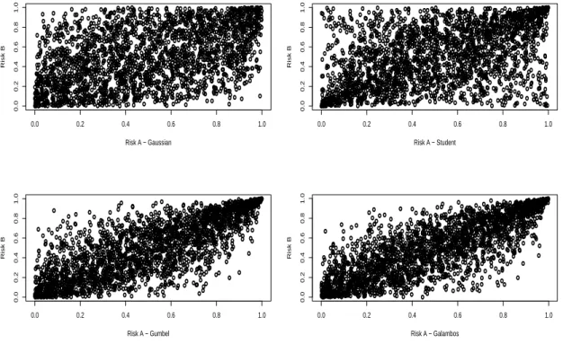
Many copulas have been studied in the literature. Because of their properties, some of them are widely used in Finance and Insurance. The current crisis highlighted the necessity for banks to consider the previous methodologies, as even if incidents of small magnitude are independent, large events tends to occur simultaneously e.g. a rogue trading (operational risks) is mechanically correlated to market risks, and may triggers a liquidity risk (Kerviel incident). The latter usually engenders a credit crunch. Consequently, practitioners should be interested in copula capturing upper tail dependencies such as the Galambos or the Gumbel copula. Figure 1 illustrates those properties and compare them to more traditional structure, for instance the Gaussian and the Student ones.

2.3 Risk measures

Initially risks in the banks were evaluated using the standard deviation applied to various asset portfolios. Nowadays, the financial industry moved to quantile-based downside risk measures

such as the Value-at-Risk (V aRα for confidence level α) and Expected Shortfall. The V aRα

measures the losses that may be expected for a given probability, and corresponds to the quan-tile of the distribution which characterizes the asset or the type of events for which the risk has to be measured. Thus, the fit of an adequate distribution to the risk factor is definitively an

● ● ● ● ● ● ● ● ● ● ● ● ● ● ● ● _● ● ● ● ● ● ● ● ● ● ● ● ● ● ● ● ● ● ● ● ● ● ● ● ● ● ● ● ● ● ● ● ● ● ● ● ● ● ● ● ● ● ● ● ● ● ● ● ● ● ● ● ● ● ● ● ● ● ● ● ● ● ● ● ● ● ● ● ● ● ● ● ● ● ● ● ● ● ● ● ● ● ● ● ● ● ● ● ● ● ● ● ● ● ● ● ● ● ● ● ● ● ● ● ● ● ● ● ● ● ● ● ● ● ● ● ● ● ● ● ● ● ● ● ● ● ● ● ● ● ● ●● ● ● ● ● ● ● ● ● ● ● ● ● ● ● ● ● ● ● ● ● ● ● ● ● ● ● ● ● ● ● ● ● ● ● ● ● ● ● ● ● ● ● ● ● ● ● ● ● ● ● ● ● ● ● ● ● ● ● ● ● ● ● ● ● ● ● ● ● ● ● ● ● ● ● ● ● ● ● ● ● ● ● ● ● ● ● ● ● ● ● ● ● ● ● ● ● ● ● ● ● ● ● ● ● ● ● ● ● ● ● ● ● ● ● ● ● ● ● ● ● ● ● ● ● ● ● ● ● ● ● ● ● ● ● ● ● ● ● ● ● ● ● ● ● ● ● ● ● ● ● ● ● ● ● ● ● ● ● ● ● ● ● ● ● ● ● ● ● ● ● ● ● ● ● ● ● ● ● ● ● ● ● ● ● ● ● ● ● ● ● ● ● ● ● ● ● ● ● ● ● ● ● ● ● ● ● ● ● ● ● ● ● ● ● ● ● ● ● ● ● ● ● ● ● ● _● ● ● ● ● ● ● ● ● ● ● ● ● ● ● ● ● ● ● ● ● ● ● ● ● ● ● ● ● ● ● ● ● ● ● ● ● ● ● ● ● ● ● ● ● ● ● ● ● ● ● ● ● ● ● ● ● ● ● ● ● ● ● ● ● ● ● ● ● ● ● ● ● ● ● ● ● ● ● ●● ● ● ● ● ● ● ● ● ● ● ● ● ● ● ● ● ● ● ● ● ● ● ● ● ● ● ● ● ● ● ● ● ● ● ● ● ● ● ● ● ● ● ● ● ● ● ● ● ● ● ● ● ● ● ● ● ● ● ● ● ● ● ● ● ● ● ● ● ● ● ● ● ● ● ● ● ● ● ● ● ● ● ● ● ● ● ● ● ● ● ● ● ● ● ● ● ● ● ● ● ● ● ● ● ● ● ● ● ● ● ● ● ● ● ● ● ● ● ● ● ● ● ● ● ● ● ● ● ● ● ● ● ● ● ● ● ● ● ● ● ● ● ● ● ● ● ● ● ● ● ● ● ● ● ● ● ● ● ● ● ● ● ● ● ● ● ● ● ● ● ● ● ● ● ● ● ● ● ● ● ● ● ● ● ● ● ● ● ● ● ● ● ● ● ● ● ● ● ● ● ● ● ● ● ● ● ● ● ● ● ● ● ● ● ● ● ● ● ● ● ● ● ● ● ● ● ● ● ● ● ● ● ● ● ● ● ● ● ● ● ● ● ● ● ● ● ● ● ● ● ● ● ● ● ● ● ● ● ● ● ● ● ● _● ● ● ● ● ● ● ● ● ● ● ● ● ● ● ● ● ● ● ● ● ● ● ● ● ● ● ● ● ● ● ● ● ● ● ● ● ● ● ● ● ● ● ● ● ● ● ● ● ● ● ● ● ● ● ● ● ● ● ● ● ● ● ● ● ● ● ● ● ● ● ● ● ● ● ● ● ● ● ● ● ● ● ● ● ● ● ● ● ● ● ● ● ● ● ● ● ● ● ● ● ● ● ● ● ● ● ● ● ● ● ● ● ● ● ● ● ● ● ● ● ● ● ● ● ● ● ● ● ● ● ● ● ● ● ● ● ● ● ● ● ● ● ● ● ● ● ● ● ● ● ● ● ● ● ● ● ● ● ● ● ● ● ● ● ● ● ● ● ● ● ● ● ● ● ● ● ● ● ● ● ● ● ● ● ● ● ● ● ● ● ● ● ● ● ● ● ● ● ● ● ● ● ● ● ● ● ● ● ● ● ● ● ● ● ● ● ● ● ● ● ● ● ● ● ● ● ● ● ● ● ● ● ● ● ● ● ● ● ● ● ● ● ● ● ● ● ● ● ● ● ● ● ● ● ● ● ● ● _● ● ● ● ● ● ● ● ● ● ● ● ● ● ● ● ● ● ● ● ● ● ● ● ● ● ● ● ● ● ● ● ● ● ● ● ● ● ● ● ● ● ● ● ● ● ● ● ● ● ● ● ● ● ● ● ● ● ● ● ● ● ● ● ● ● ● ● ● ● ● ● ● ● ● ● ● ● ● ● ● ● ● ● ● ● ● ● ● ● ● ● ● ● ● ● ● ● ● ● ● ● ● ● ● ● ● ● ● ● ● ● ● ● ● ● ● ● ● ● ● ● ● ● ● ● ● ● ● ● ● ● ● ● ● ● ● ● ● ● ● ● ● ● ● ● ● ● ● ● ● ● ● ● ● ● ● ● ● ● ● ● ● ● ● ● ● ● ● ● ● ● ● ● ● ● ● ● ● ● ● ● ● ● ● ● ● ● ● ● ● ● ● ● ● ● ● ● ● ● ● ● ● ● ● ● ● ● ● ● ● _● ● ● ● ● ● ● ● ● ● ● ● ● ● ● ● ● ● ● ● _● ● ● ● ● ● ● ● ● ● ● ● ● ● ● ● ● ● ● ● ● ● ● ● ● ● ● ● ● ● ● ● ● ● ● ● ● ● ● ● ● ● ● ● ● ● ● ● ● ● ● ● ● ● ● ● ● ● ● ● ● ● ● ● ● ● ● ● ● ● ● ● ● ● ● ● ● ● ● ● ● ● ● ● ● ● ● ● ● ● ● ● ● ● ● ● ● ● ● ● ● ● ● ● ● ● ● ● ● ● ● ● ● ● ● ● ● ● ● ● ● ● ● ● ● ● ● ● ● ● ● ● ● ● ● ● ● ● ● ● ● ● ● ● ● ● ● ● ● ● ● ● ● ● ● ● ● ● ● ● ● ● ● ● ● ● ● ● ● ● ● ● ● ● ● ● ● ● ● ● ● ● ● ● ● ● ● ● ● ● ● ● ● ● ● ● ● ● ● ● ● ● ● ● ● ● ● ● ● ● ● ● ● ● ● ● ● ● ● ● ● ● ● ● ● ● ● ● ● ● ● ● ● ● ● ● ● ● ● ● ● ● ● ● ● ● ● ● ● ● ● ● ● ● ● ● ● ● ● ● ● ● ● ● ● ● ● ● ● ● ● ● ● ● ● ● ● ● ● ● ● ● ● ● ● ● ● ● ● ● ● ● ● ● ● ● ● ● ● ● ● ● ● ● ● ● ● ● ● ● ● ● ● ● ● ● ● ● ● ● ● ● ● ● ● ● ● ● ● ● ● ● ● ● ● ● ● ● ● ● ● ● ● ● ● ● ● ● ● ● ● ● ● ● ● ● ● ● ● ● ● ● ● ● ● ● ● ● ● ● ● ● ● ● ● ● ● ● ● ● ● ● ● ● ● ● ● ● ● ● ● ● ● ● ● ● ● ● ● ● ● ● ● ● ● ● ● ● ● ● ● ● ● ● ● ● ● ● ● ● ● ● ● ● _● ● ● ● ● ● ● ● ● ● ● ● ● ●● ● ● ● ● ● ● ● ● ● ● ● ● ● ● ● ● ● ● ● ● ● ● ● ● ● ● ● ● ● ● ● ● ● ● ● ● ● ● ● ● ● ● ● ● ● ● ● ● ● ● ● ● ● ● ● ● ● ● ● ● ● ● ● ● ● ● ● ● ● ● ● ● ● ● ● ● ● ● ● ● ● ● ● ● ● ● ● ● ● ● ● ● ● ● ● ● ● ● ● ● ● ● ● ● ● ● ● ● ● ● ● ● ● ● ● ● ● ● ● ● ●● ● ● ● ● ● ● ● ● ● ● ● ● ● ● ● ● ● ● ● ● ● ● ● ● ● ● ● ● ● ● ● ● ● ● ● ● ● ● ● ● ● ● ● ● ● ● ● ● ● ● ● ● ● ● ● ● ● ● ● ● ● ● ● ● ● ● ● ● ● ●● _● ● ● ● ● ● ● ● ● ● ● ● ● ● ● ● ● ● ● ● ● ● ● ● ● ● ● ● ● ● ● ● ● ● ● ● ● ● ● ● ● ● ● ● ● ● ● ● ● ● ● ● ● ● ● ● ● ● ● ● ● ● ●● ● ● ● ● ● ● ● ● ● ● _● ● ● ● ● ● ● ● ● ● ● ● ● ● ● ● ● ● ● ● ● ● _● ● ● ● ● ● ● ● ● ● ● ● ● ● ● ● ● ● ● ● ● ● ● ● ● ● ● ● ● ● ● ● ● ● ● ● ● ● ● ● ● ● ● _● ● ● ● ● ● ● ● ● ● ● ● ● ● ● ● ● ● ● ● ● ● ● ● ● ● ● ● ● ● ● ● ● ● ● ● ● ● ● ● ● ● ● ● ● ● ● ● ● ● ● ● ● ● ● ● ● ● ● ● ● ● ● ● ● ● ● ● ● ● ● ● ● ● ● ● ● ● ● ● ● ● ● ● ● ● ● ● ● ● ● ● ● ● ● ● ● ● ● ● ● ● ● ● ● ● ● ● ● ● ● ● ● ● ● ● ● ● ● ● ● ● ● ● ● ● ● ● ● ● ● ● ● ● ● ● ● ● ● ● ● ● ● ● ● ● ● ● ● ● ● ● ● ● ● ● ● ● ● ● ● ● ● ● ● ● ● ● ● ● ● ● ● ● ● ● ● ● ● ● ● ● ● ● ● ● ● ● ● ● ● ● ● ● ● ● ● ● ● ● ● ● ● ● ● ● ● ● ● ● ● ● ● ● ● ● ● ● ● ● ● ● ● ● ● ● ● ● ● ● ● ● ● ● ● ● ● ● ● ● ● ● ● ● ● ● ● ● ● ● _● ● ● ● ● ● ● ● ● ● ● ● ● ● ● ● ● ● ● ● ● ● ● ● ● ● ● ● ● ● ● ● ● ● ● ● ● ● ● ● ● ● ● ● ● ● ● ● ● ● ● ● ● ● ● ● ● ● ● ● ● ● ● ● ● ● ● ● ● ● ● ● ● ● ● ● ● ● ● ● ● ● ● ● ● ●● ● ● ● ● ● ● ● ● ● ● ● ● ● ● ● ● ● ● ● ● ● ● ● ● ● ● ● ● ● ● ● ● ● ● ● ● ● ● ● ● ● ● ● ● ● ● ● ● ● ● ● ● ● ● ● ● ● ● ● ● ● ● ● ● ● ● ● ● ● ● ● ● ● ● ● ● ● ● ● ● ● ● ● ● ● ● ● ● ● ● ● ● ● ● ● ● ● ● ● ● ● ● ● ● ● ● ● ● ● ● ● ● ● ● ● ● ● ● ● ● ● ● ● ● ● ● ● ● ● ● ● ● ● ● _● ● ● ● ● ● ● ● ● ● ● ● ● ● ● ● ● ● ● ● ● ● ● ● ● ● ● ● ● ● ● ● ● ● ● ● ●● ● ● ● ● ● ● ● ● ● ● ● ● 0.0 0.2 0.4 0.6 0.8 1.0 0.0 0.2 0.4 0.6 0.8 1.0 Risk A − Gaussian Risk B ● ● ● ● ● ● ● ● ● ● ● ● ● ● ● ● ● ● ● ● ● ● ● ● ● ● ● ● ● ● ● ● ● ● ● ● ● ● ● ● ● ● ● ● ● ● ● ● ● ● ● ● ● ● ● ● ● ● ● ● ● ● ● ● ● ● _● ● ● ● ● ● ● ● ● ● ● ● ● ● ● ● ● ● ● ● ● ● ● ● ● ● ● ● ● ● ● ● ● ● ● ● ● ● ● ● ● ● ● ● ● ● ● _● ● ● ● ● ● ● ● ● ● ● ● ● ● ● ● ● ● ● ● ● ● ● ● ● ● ● ● ● ● ● ● ●● ● ● ● ● ● ● ● ● ● ● ● ● ● ● ● ● ● ● ● ● ● ● ● ● ● ● ● ● ● ● ● ● ● ● ● ● ● ● ● ● ● ● ● ● ● ● ● ● ● ● ● ● ● ● ● ● ● ● ● ● ● ● ● ● ● ● ● ● ● ● ● ● ● ● ● ● ● ● ● ● ● ● ● ● ● ● ● ● ● ● ● ● ● ● ● ● ● ● ● ● ● ● ● ● ● ● ● ● ● ● ● ● ● ● ● ● ● ● ● ● ● ● ● ● ● ● ●● ● ● ● ● ● ● ● ● ● ● ● ● ● ● ● ● ● ● ● ● ● ● ● ● ● ● ● ● ● ● ● ● ● ● ● ● ● ● ● ● ● ● ● ● ● ● ● ● ● ● ● ● ● ● ● ● ● ● ● ● ● ● ● ● ● ● ● ● ● ● ● ● ● ● ● ● ● ● ● ● ● ● ● ● ● ● ● ● ● ● ● ● ● ● ● ● ● ● ● ● ● ● ● ● ● ● ● ● ● ● ● ● ● ● ● ● ● ● ● ● ● ● ● ● ● ● ● ● ● ● ● ● ● ● ● ● ● ● ● ● ● ● ● ● ● ● ● ● ● ● ● ● ● ● ● ● ● ● ● ● ● ● ● ● ● ● ● ● ● ● ● ● ● ● ● ● ● ● ● ● ● ● ● ● ● ● ● ● ● ● ● ● ● ● ● ● ● ● ● ● ● ● ● ● ● ● ● ● ● ● ● ● ● ● ● ● ● ● ● ● ● ● ● ● ● ● ● ● ● ● ● ● ● ● ● ● ● ● ● ● ● ● ● ● ● ● ● ● ● ● ● ● ● ● ● ● ● ● ● ● ● ● ● ● ● ● ● ● ● ● ● ● ● ● ● ● ● ● ● ● ● ● ● ● ● ● ● ● ● ● ● ● ● ● ● ● ● ● ● ● ● ● ● ● ● ● ● ● ● ● ● ● ● ● ● ● ● ● ● _● ● ● ● ● ● ● ● ● ● ● ● ● ● ● ● ● ● ● ● _● ● ● ● ● ● ● ● ● ● ● ● ● ● ● ● ● ● ● ● ● ● ● ● ● ● ● ● ● ● ● ● ● ● ● ● ● ● ● ● ● ● ● ● ● ● ● ● ● ● ● ● ● ● ● ● ● ● ● ● ● ● ● ● ● ● ● ● ● ● ● ● ● ● ● ● ● ● ● ● ● ● ● ● ● ● ● ● ● ● ● ● ● ● ● ● ● ● ● ● ● ● ● ● ● ● ● ● ● ● ● ● ● ● ● ● ● ● ● ● ● ● ● ● ● ● ● ● ● ● ● ● ● ● ● ● ● ● ● ● ● ● ● ● ● ● ● ● ● ● ● ● ● ● ● ● ● ● ● ● ● ● ● ● ● ● ● ● ● ● ● ● ● ● ● ● ● ● ● ● ● ● ● ● ● ● ● ● ● ● ● ● ● ● ● ● ● ● ● ● ● ● ● ● ● ● ● ● ● ● ● ● ● ● ● ● ● ● ● ● ● ● ● ● ● ● ● ● ● ● ● ● ● ● ● ● ● ● ● ● ● ● ● ● ● ● ● ● ● ● ● ● ● ● ● ● ● ● ● ● ● ● ● ● ● ● ● ● ● ● ● ● ● ● ● ● ● ● ● ● ● ● ● ● ● ● ● ● ● ● ● ● ● ● ● ● ● ● ● ● ● ● ● ● ● ● ● ● ● ● ● ● ● ● ● ● ● ● ● ● ● ● ● ● ● ● ● ● ● ● ● ● ● ● ● ● ● _● ● ● ● ● ● ● ● ● ● ● ● ● ● ● ● ● ● ● ● ● ● ● ● ● ● ● ● ● ● ● ● ● ● ● ● ● ● ● ● ● ● ● ● ● ● ● ● ● ● ● ● ● ● ● ● ● ● ● ● ● ● ● ● ● ● ● ● ● ● _● ● ● ● ● ● ● ● ● ● ● ● ● ● ● ● ● ● ● ● ● ● ● ● ● ● ● ● ● ● ● ● ● ● ● ● ● ● ● ● ● ● ● ● ● ● ● ● ● ● ● ● ● ● ● ● ● ● ● ● ● ● ● ● ● ● ● ● ● ● ● ● ● ● ● ● ● ● ● ● ● ● ● ● ● ● ● ● ● ● ● ● ● ● ● ● ● ● ● ● ● ● ● ● ● ● ● ● ● ● ● ● ● ● ● ● ● ● ● ● ● ● ● ● ● ● ● ● ● ● ● ● ● ● ● ● ● ● ● ● ● ● ● ● ● ● ● ● ● ● ● ● ● ● ● ● ● ● ● ● ● ● ● ● ● ● ● ● ● ● ● ● ● ● ● ● ● ● ● ● ● ● ● ● ● ●● ● ● ● ● ● ● ● ● ● ● ● ● ● ● ● ● ● ● ● ● ● ● ● ● ● ● ● ● ● ● ● ● ● ● ● ● ● ● ● ● ● ● ● ● ● ● ● ● ● ● ● ● ● ● ● ● ● ● ● ● ● ● ● ● ● ● ● ● ● ● ● ● ● ● ● ● ● ● ● ● ● ● ● ● ● ● ● ● ● ● ● ● ● ● ● ● ● ● ● ● ● ● ● ● ● ● ● ● ● ● ● ● ● ● ● ● ● ● ● ● ● ● ● ● ● ● ● ● ● ● ● ● ● ● ● ● ● ● ● ● ● ● ● ● ● ● ● ● ● ● ● ● ● ● ● ● ● ● ● ● ● ● ● ● ● ● ● ● ● ● ● ● ● ● ● ● ●● ● ● ● ● ● ● ● ● ● ● ● ● ● ● ● ● ● ● ● ● ● ● ● ● ● ● ● ● ● ● ● ● ● ● ● ● ● ● ● ● ● ● ● ● ● ● ● ● ● ● ● ● ● ● ● ● ● ● ● ● ● ● ● ● ● ● ● ● ● ● ● ● ● ● ● ● ● ● ● ● ● ● ● ● ● ● ● ● ● ● ● ● ● ● ● ● ● ● ● ● ● ● ● ● ● ● ● ● ● ● ● ● ● ● ● ● ● ● ● ● ● ● ● ● ● ● ● ● ● ● ● ● ● ● ● ● ● ● ● ● ● ● ● ● ● ● ● ● ● ● ● ● ● ● ● ● ● ● ● ● ● ● ● ● ● ● ● ● ● ● ● ● ● ● ● ● ● ● ● ● ● ● ● ● ● ● ● ● ● ● ● ● ● ● ● ● ● ● ● ● ● ● ● ● ● ● ● ● ● ● ● ● ● ● ● ● ● ● ● ● ● ● ● ● ● ● ● ● ● ● ● ● ● ● ● ● ● ● ● ● ● ● ● ● ● ● ● ● ● ● ● ● ● ● ● ● ● ● ● ● ● ● ● ● ● ● ● ● ● ● ● ● ● ● ● ● ● ● ● ● ● ● ● ● ● ● ● ● ● ● ● ● ● ● ● ● ● ● ● ● ● ● ● ● ● ● ● ● ● ● ● ● ● ● ● ● ● ● ● ● ● ● ● ● ● ● ● ● ● ● ● ● ● ● ● ● ● ● ● ● ● ● ● ● ● ● ● ● ● ● ● ● ● ● ● ● ● ● ● ● ● ● ● ● ● ● ● ● ● ● ● ● ● ● ● ● ● ● ● ● ● ● ● ● ● ● ● ● ● ● ● ● ● ● ● ● ● ● ● ● ● ● ● ● ● ● ● ● ● ● ● ● ● _● ● ● ● ● ● ● ● ● ● ● ● ● ● ● ● ● ● ● ● ● ● ● ● ● ● ● ● ● ● ● ● ● ● ● ● ● ● ● ● ● ● ● ● ● ● ● ● ● ● ● ● ● ● ● ● ● ● ● ● ● ● _● ● _● ● ● ● ● ● ● ● ● _● ● ● ● ● ● ● ● ● ● ● ● ● ● ● ● ● ● ● ● ● ● ● ● ● ● ● ● ● ● ● ●● ● ● ● ● ● ● ● ● ● ● ● ● ● ● ● ● ● ● ● ● ● ● ● ● ● ● ● ● ● ● ● ● ● ● ● ● ● ● ● ● ● ● ● ● ● ● ● ● ● ● ● ● ● ● ● ● ● ● ● ● ● ● ● ● ● ● ● ● ● ● ● ● ● ● ● ● ● ● ● ● ● ● ● ● ● ● ● ● ● ● ● ● ● ● ● ● ● ● ● ● ● ● ● ● ● ● ● ● ● ● ● ● ● ● ● ● ● ● ● ● ● ● ● ● ● ● ● ● ● ● ● ● ● ● ● ● ● ● ● ● ● ● ● ● ● ● ● ● ● ● ● ● ● ● ● ● ● ● ● ● ● ● ● ● ● ● ● ● ● ● ● ● ● ● ● ● ● ● ● ● ● ● ● ● ● ● ● ● ● ● ● ● ● ● ● ● ● ● ● ● ● ● ● ● ● ● ● ● ● ● ● ● ● ● ● ● ● ● ● ● ● ● ● ● ● ● ● ● ● ● ● ● ● ● ● ● ● ● ● ● ● ● ● ● ● ● ● ● ● ● ● ● ● ● ● ● ● ● ● ● ● ● ● ● ● ● ● ● ● ● ● ● ● _● ● ● ● ● ● ● ● ● ● ● ● ● ● ● ● ● ● ● ● ● ● ● ● ● ● ● ● ● ● ● ● ● ● ● ● ● ● ● ● ● ● ● ● ● ● ● ● ● ● ● ● ● ● ● ● ● ● ● ● ● ● ● ● ● ● ● ● ● ● ● ● ● ● ● ● ● ● ● ● ● ● ● ● ● ● ● ● ● ● ● ● ● ● ● ● ● ● ● ● ● ● ● ● ● ● ● ● ● ● ● ● ● ● ● ● ● ● ● ● ● ● ● ● ● ● ● ● ● ● ● ● ● ● ● ● ● ● ● ● ● ● ● ● ● ● ● ● ● ● ● ● ● ● ● ● ● ● ● ● ● ● ● ● ● ● ● ● ● ● ● ● ● ● ● ● ● ● ● ● ● ● ● ● ● ● ● ● ● ● ● ● ● ● ● ● ● ● ● ● ● ● ● ● ● ● ● ● ● ● ● ● ● ● ● ● ● ● ● ● ● ● ● ● ●● ● ● ● ● ● ● ● ● ● ● ● ● ● ● ● ● ● ● ● ● ● ● ● ● ● ● ● ● ● ● ● ● ● ● ● _● ● ● ● ● ● ● ● ● ● ● ● ● ● ● ● ● ● ● ● ● ● ● ● ● ● ● ● ● ● ● ● ● ● ● ● ● ● ● ● ● ● ● ● ● ● ● ● ● ● ● ● ● ● ● ● ● ● ● ● ● 0.0 0.2 0.4 0.6 0.8 1.0 0.0 0.2 0.4 0.6 0.8 1.0 Risk A − Student Risk B ● ● ● ● ● ● ● ● ● ● ● ● ● ● ● ● ● ● ● ● ● ● ● ● ● ● ● ● ● ● ● ● ● ● ● ● ● ● ● ● ● ● ● ● ● ● ● ● ● ● ● ● ● ● ● ● ● ● ● ● ● ● ● ● ● ● ● ● ● ●_● ● ● ● ● ● ● ● ● ● ● ● ● ● ● ● ● ● ● ● ● ● ● ● ● ● ● ● ● ● ● ● ● ● ● ● ● ● ● ● ● ● ● ● ● ● ● ● ● ● ● ● ● ● ● ● ● ● ● ● ● ● ● ● ● ● ● ● ● ● ● ● ● ● ● ● ● ● ● ● ● ● ● ● ● ● ● ● ● ● ● ● ● ● ● ● ● ● ● ● ● ● ● ● ● ● ● ● ● ●_● ● ● ● ● ● ● ● ● ● ● ● ● ● ● ● ● ● ● ●● ● ● ● ● ● ● ● ● ● ● ● ● ● ● ● ● ● ● ● ● ● ● ● ● ● ● ● ● ● ● ● ● ● ● ● ● ● ● ● ● ● ● ● ● ● ● ● ● ● ● ● ● ● ● ● ● ● ● ● ● ● ● ● ● ● ● ● ● ● ● ● ● ● ● ● ● ● ● ● ● ● ● ● ● ● ● ● ● ● ● ● ● ● ● ● ● ● ● ● ● ● ● ● ● ● ● ● ● ● ● ● ● ● ● ● ● ● ● ● ● ● ● ● ● ● ● ● ● ● ●● ● ● ● ● ● ● ● ● ● ● ● ● ● ● ● ● ● ● ● ● ● ● ● ● ● ● ● ● ● ● ● ● ● ● ● ● ● ● ● ● ● ● ● ● ● ● ● ● ● ● ● ● ● ● ● ● ● ● ● ● ● ● ● ● ● ● ● ● ● ● ● _● ● ● ● ● ● ● ● ● ● ● ● ● ● ● ● ● ● ● ● ● ● ● ● ● ● ● ● ● ● ● ● ● ● ● ● ● ● ● ● ● ● ● ● ● ● ● ● ● ● ●● ● ● ● ● ● ● ● ● ● ● ●● ● ● ● ● ● ● ● ● ● ● ● ● ● ● ● ● ● ● ● ● ● ● ● ● ● ● ● ● ● ● ● ● ● ● ● ● ● ● ● ● ● ● ● ● ● ● ● ● ● ● ● ● ● ● ● ● ● ● ● ● ● ● ●● ● ● ● ● ● ● ● ● ● ● ● ● ● ● _● ● ● ● ● ● ● ● ● ● ● ● ● ● ● ● ● ● ● ● ● ● ● ● ● ● ● ● ● ● ● ● ● ●● ● ● ● ● ● ● ● ● ● ● ● ● ● ● ● ● ● ● ● ● ● ● ● ● ● ● ● ● ● ● ● ● ● ● ● ● ● ● ● ● ● ● ● ● ● ● ● ● ● ● ● ● ● ● ● ● ● ● ● ● ● ● ● ● ● ● ● ● ● ● ● ● ● ● ● ● ● ● ● ● ● ● ● ● ● ● ● ● ● ● ● ● ● ● ● ● ● ● ● ● ● ● ● ● ● ● ● ● ● ● ● ● ● ● ● ● ● ● ● ● ● ● ● ● ● ● ● ● ● ● ● ● ● ● ● ● ● ● ● ● ● ● ● ● ● ● ● ● ● ● ● ● ● ● ● ● ● ● ● ● ● ● ● ● ● ● ● ● ● ● ● ● ● ● ● ● ● ● ● ● ● ● ● ● ● ● ● ● ● ● ● ● ● ● ● ● ● ● ● ● ● ● ● ● ● ● ● ● ● ● ● ● ● ● ● ● ● ● ● ● ● ● ● ● ● ● ● ● ● ● ● ● ● _● ● ● ● ● ● ● ● ● ● ● ● ● ● ● ● ● ● ● ● ● ● ● ● ● ● ● ● ● ● ● ● ● ● ● ● ● ● ● ● ● ● ● ● ● ● ● ● ● ● ● ● ● ● ● ● ● ● ● ● ● ● ● ● ● ● ● ● ● ● ● ● ● ● ● ● ● ● ● ● ● ● ● ● ● ● ● ● ● ● ● ● ● ● ● ● ● ● ● ● ● ● ● ● ● ● ● ● ● ● ● ● ● ● ● ● ● ● ● ● ● ● ● ● ● ● ● ● ● ● ● ● ● ● ● ● ● ● ● ● ● ● ● ● ● ● ● ● ● ● ● ● ● ● ● ● ● ● ● ● ● ● ● ● ● ● ● ● ● ● ● ● ● ● ● ● ● ● ● ● ● ● ● ● ● ● ● ● ● ● ● ● ● ● ● ● ● ● ● ● ● ● ● ● ● ● ● ● ● ● ● ● ● ● ● ● ● ● ● ● ● ● ● ● ● ● ● ● ● ● ● ● ● ● ● ● ● ● ● ● ● ● ● ● ● ● ● ● ● ● ● ● ● ● ● ● ● ● ● ● ● ● ● ● ● ● ● ● ● ● ● ● ● ● ● ● ● ● ● ● ● ● ● ● ● ● ● ● ● ● ● ● ● ● ● ● ● ● ● ● ● ● ● ● ● ● ● ● ● ● ● ● ● ● ● ● ● ● ● ● ● ● ● ● ● ● ● ● ● ● ● ● ● ● ● ● ● ● ● ● ● ● ● ● ● ● ● ● ● ● ● ● ● ● ● ● ● ● ● ● ● ● ● ● ● ● ● ●● ● ● ● ● ● ● ● ● ● ● ● ● ● ● ● ● ● ● ● ● ● ● ● ● ● ● ● ● ● ● ● ● ● ● ● ● ● ● ● ● ● ● ● ● ● ● ● ● ● ● ● ● ● ● ● ● ● ● ● ● ● ● ● ● ● ● ● ● ● ● ● ● ● ● ● ● ● ● ● ● ● ● ● ● ● ● ● ● ● ● ● ● ● ● ● ● ● ● ● ● ● ● ● ● ● ● ● ● ● ● ● ● ● ● ● ● ● ● ● ● ● ● ● ● ● ● ● ● ● ● ● ● ● ● ● _● ● ● ● ● ● ● ● ● ● ● ● ● ● ● ● ● ● ● ● ● ● ● ● ● ● ● ● ● ● ● ● ● ● ● ● ● ● ● ● ● ● ● ● ● ● ● ● ●● ● ● ● ● ● ● ● ● ● ● ● ● ● ● ● ● ● ● ● ● ● ● ● ● ● ● ● ● ● ● ● ● ● ● ● ● ● ● ● ● ● ● ● ● ● ● ● ● ● ● ● ● ● ● ● ● ● ● ● ● ● ● ● ● ● ● ● ● ● ● ● ● ● ● ● ● ● ● ● ● ● ● ● ● ● ● ● ● ● ● _● ● ● ● ● ● ● ● ● ● ● ● ● ● ● ● ● ● ● ● _● ● ● ● ● ● ● ● ● ● ● ● ● ● ● ● ● ● ● ● ● ● ● ● ● ● ● ● ● ● ● ● ● ● ● ● ● ● ● ● ● ● ● ● ● ● ● ● ● ● ● ● ● ● ● ● ● ● ● ● ● ● ● ● ● ● ● ● ● ● ● ● ● ● ● ● ● ● ● ● ● ● ● ● ● ● ● ● ● ● ● ● ● ● ● ● ● ● ● ● ● ● ● ● ● ● ● ● ● ● ● ● ● ● ● ● ● ● ● ● ● ● ● ● ● ● ● ● ● ● ● ● ● ● ● ● ● ● ● ● ● ● ● ● ● ● ● ● ● ● ● ● ● ● ● ● ● ● ● ● ● ● ● ● ● ● ● ● ● ● ● ● ● ● ● ● ● ● ● ● ● ● ● ● ● ● ● ● ● ● ● ● ● ● ● ● ● ● ● ● ● ● ● ● ● ● ● ● ● ●● ● ● ● ● ● ● ● ● ● ● ● ● ● ● ● ● ● ● ● ● ● ● ● ● ● ● ● ● ● ● ● ● ● ● ● ● ● ● ● ● ● ● ● ● ● ● ● ● ● ● ● ● ● ● ● ● ● ● ● ● ● ● ● ● ● ● ● ● ● ● ● ● ● ● ● ● ● ● ● ● ● ● _● ● ● ● ● ● ● ● ● ● ● ● ● ● ● ● ● ● ● ● ● ● ● ● ● ● ● ● ● ● ● ● ● ● ● ● ● ● ● ● ● ● ● ● ● ● ● ● ● ● ● ● ● ● ● ● ● ● ● ● ● ● ● ● ● ● ● ● ● ● ● ● ● ● ● ● ● ● ● ● ● ● ● ● ● ● ● ● ● ● ● ● ● ● ● ● ● ● ● ● ● ● ● ● ● ● ● ● ● ● ● ● ● ● ● ● ● ● ● ● ● ● ● ● ● ● ● ● ● ● ● ● ● ● ● ● ● ● ● ● ● ● ● ● ● ● ● ● ● ● ● ● ● ● ● ● ● ● ● ● ● ● ● ● ● ● ● ● ● ● ● ● ● ● ● ● ● ● ● ● ● ● ● ● ● ● ● ● ● ● ● ● ● ● ● ● ● ● ● ● ● ● ● ● ● ● ● ● ● ● ● ● ● ● ● ● ● ● ●● ● ● ● ● ● ● ● ● ● ● ● ● ● ● ● ● ● ● ● ● ● ● ● ● ● ● ● ● ● ● ● ● ● ● ● ● ● ● ● ● ● ● ● ● ● ● ● ● ● ● ● ● ● ● ● ● ● ● ● ● ● ● ● ● ● ● ● ● ● ● ● ● ● ● ● ● ● ● ● ● ● ● ● ● ● ● ● ● ● ● ● ● ● ● ● ● ● ● ● ● ● ● ● ● ● ● ● ● ● ● ● ● ● ● ● ● ● ● ● ● ● ● ● ● ● ● ● ● ● ● ● ● ● ● ● ● ● ● ● ● ● ● ● ● ● ● ● ● ● ● ● ● ● ● ● ● ● ● ● _● ● ● ● ● ● ● ● ● ● ● ● ● ● ● ● ● ● ● ● ● ● ● ● ● ● ● ● ● ● ● ● ● ● ● ● ● ● ● ● ● ● ● ● ● ● ● ● ● ● ● ● ● ● ● ● ● ● ● ● ● ● ● ● ● ● ● ● ● ● ● ● ● ● ● ● ● ● ● ● ● ● ● ● ● ● ● ● ● ● ● ● ● ● ● ● ● ● ● ● ● ● ● ● ● ● ● ● ● ● ● ● ● ● ● ● ● ● ● ● ● ● ● ● ● ● ● ● ● ● ● ● ● ● ● ● ● ● ● ● ● ● ● ● ● ● ● ● ● ● ● ● ● ● ● ● ● ● ● ● ● ● ● ● ● ● ● ● ● ● ● ● ● ● ● ● ● ● ● ● ● ● ● ● ● ● ● ● ● ● ● ● ● ● ● ● ● ● ● ● ● ● ● ● ● ● ● ● ● ● ● ● ● ● ● ● ● ● ● ● ● ● ● ● ● ● ● ● ● ● ● ● ● ● ● ● ● ● ● ● ● ● ● ● ● ● ● ● ● ● ● ● ● ● ● ● ● ● ● ● ● ● ● ● ● ● ● ● ● ● ● ● ● ● ● ● ● ● ● ● ● ● ● ● ● ● ● ● ● ● ● ● ● ● ● ● ● ● ● ● ● ● ● ● ● ● ● ● ● ● ● ● ● ● ● ● ● ● ● ● ● ● ● ● ● ● ● ● ● ● ● ● ● ● ● ● ● ● ● ● ● ● ● ● ● ● ● ● ● ● ● 0.0 0.2 0.4 0.6 0.8 1.0 0.0 0.2 0.4 0.6 0.8 1.0 Risk A − Gumbel Risk B ● ● ● ● ● ● ● ● ● ● ● ● ● ● ● ● ● ● ● ● ● ● ● ● ● ● ● ● ● ● ● ● ● ● ● ● ● ● ● ● ● ● ● ● ● ● ● ● ● ● ● ● ● ● ● ● ● ● ● ● ● ● ● ● ● ● ● ● ● ● ● ● ● ● ● ● ● ● ● ● ● ● ● ● ● ● ● ● ● ● ● ● ● ● ● ● ● ● ● ● ● ● ● ● ● ● ● ● ● ● ● ● ● ● ● ● ● ● ● ● ● ● ● ● ● ● ● ● ● ● ● ● ● ● ● ● ● ● ● ● ● ● ● ● ● ● ● ● ● ● ● ● ● ● ● ● ● ● ● ● ● ● ● ● ● ● ● ● ● ● ● ● ● ● ● ● ● ● ● ● ● ● ● ● ● ● ● ● ● ● ● ● ● ● ● ● ● ● ● ● ● ● ● ● ● ● ● ● ● ● ● ● ● ● ● ● ● ● ● ● ● ● ● ● ● ● ● ● ● ● ● ● ● ● ● ● ● ● ● ● ● ● ● ● ● ● ● ● ● ● ● ● ● ● ● ● ● ● ● ● ● ● ● ● ● ● ● ● ● ● ● ● ● ● ● ● ● ● ● ● ● ● ● ● ● ● ● ● ● ● ● ● ● ● ● ● ● ● ● ● ● ● ● ● ● ● ● ● ● ● ● ● ● ● ● ● ● ● ● ● ● ● ● ● ● ● ● ● ● ● ● ● ● ● ● ● ● ● ● ● ● ● ● ● ● ● ● ● ● ● ● ● ● ● ● ● ● ● ● ● ● ● ● ● ● ● ● ● ● ● ● ● ● ● ● ● ● ● ● ● ● ● ● ● ● ● ● ● ● ● ● ● ● ● ● ● ● ● ● ● ● ● ● ● ● ● ● ● ● ● ● ● ● ● ● ● ● ● ● ● ● ● ● ● ● ● ● ● ● ● ● ● ● ● ● ● ● ● ● ● ● ● ● ● ● ● ● ● ● ● ● ● ● ● ● ● ● ● ● ● ● ● ● ● ● ● ● ● ● ● ● ● ● ● ● ● ● ● ● ● ● ● ● ● ● ● ● ● ● ● ● ● ● ● ● ● ● ● ● ● ● ● ● ● ● ● ● ● ● ● ● ● ● ● ● ● ● ● ● ● ● ● ● ● ● ● ● ● ● ● ● ● ● ● ● ● ● ● ● ● ● ● ● ● ● ● ● ● ● ● ● ● ● ● ● ● ● ● ● ● ● ● ● ● ● ● ● ● ● ● ● ● ● ● ● ● ● ● ● ● ● ● ● ● ● ● ● ● ● ● ● ● ● ● ● ● ●● ● ● ● ● ● ● ● ● ● ● ● ● ● ● ● ● ● ● ● ● ● ● ● ● ● ● ● ● ● ● ● ● ● ● ● ● ● ● ● ● ● ● ● ● ● ● ● ● ● ● ● ● ● ● ● ● ● ● ● ● ● ● ● ● ● ● ● ● ● ● ● ● ● ● ● ● ● ● ● ● ● ● ● ● ● ● ● ● ● ● ● ● ● ● ● ● ● ● ● ● ● ● ● ● ● ● ● ● ● ● ● ● ● ● ● ● ● ● ● ● ● ● ● ● ● ● ● ● ● ● ● ● ● ● ● ● ● ● ● ● ● ● ● ● ● ● ● ● ● ● ● ● ● ● ● ● ● ● ● ● ● ● ● ● ● ● ● ● ● ● ● ● ● ● ● ● ● ● ● ● ● ● ● ● ● ● ● ● ● ● ● ● ● ● ● ● ● ● ● ● ● ● ● ● ● ● ● ● ● ● ● ● ● ● ● ● ● ● ● ● ● ● ● ● ● ● ● ● ● ● ● ● ● ● ● ● ● ● ● ● ● ● ● ● ● ● ● ● ● ● ● ● ● ● ● ● ● ● ● ● ● ● ● ● ● ● ● ● ● ● ● ● ● ● ● ● ● ● ● ● ● ● ● ● ● ● ● ● ● ● ● ● ● ● ● ● ● ● ● ● ● ● ● ● ● ● ● ● ● ● ● ● ● ● ● ● ● ● ● ● ● ● ● ● ● ● ● ● ● ● ● ● ● ● ● ● ● ● ● ● ● ● ● ● ● ● ● ● ● ● ● ● ● ● ● ● ● ● ● ● ● ● ● ● ● ● ● ● ● ● ● ● ● ● ● ● ● ● ● ● ● ● ● ● ● ● ● ● ● ● ● ● ● ● ● ● ● ● ● ● ● ● ● ● ● ● ● ● ● ● ● ● ● ● ● ● ● ● ● ● ● ● ● ● ● ● ● ● ● ● ● ● ● ● ● ● ● ● ● ● ● ● ● ● ● ● ● ● ● ● ● ● ● ● ● ● ● ● ● ● ● ● ● ● ● ● ● ● ● ● ● ● ● ● ● ● ● ● ● ● ● ● ● ● ● ● ● ● ● ● ● ● ● ● ● ● ● ● ● ● ● ● ● ● ● ● ● ● ● ● ● ● ● ● ● ● ● ● ● ● ● ● ● ● ● ● ● ● ● ● ● ● ● ● ● ● ● ● ● ● ● ● ● ● ● ● ● ● ● ● ● ● ● ● ● ● ● ● ● ● ● ● ● ● ● ● ● ● ● ● ● ● ● ● ● ● ● ● ● ● ● ● _● ● ● ● ● ● ● ● ● ● ● ● ● ● ● ● ● ● ● ● ● ● ● ● ● ● ● ● ● ● ● ● ● ● ● ● ● ● ● ● ● ● ● ● ● ● ● ● ● ● ● ● ● ● ● ● ● ● ● ● ● ● ● ● ● ● ● ● ● ● ● ● ● ● ● ● ● ● ● ● ● ● ● ● ● ● ● ● ● ● ● ● ● ● ● ● ● ● ● ● ● ● ● ● ● ● ● ● ● ● ● ● ● ● ● ● ● ● ● ● ● ● ● ● ● ● ● ● ● ● ● ● ● ● ● ● ● ● ● ● ● ● ● ● ● ● ● ● ● ● ● ● ● ● ● ● ● ● ● ● ● ● ● ● ● ● ● ● ● ● ● ● ● ● ● ● ● ● ● ● ● ● ● _● ● ● ● ● ● ● ● ● ● ● ● ● ● ● ● ● ● ● ● ● ● ● ● ● ● ● ● ● ● ● ● ● ● ● ● ● _● ● ● ● ● ● ● ● ● ● ● ● ● ● ● ● ● ● ● ● ● ● ● ● ● ● ● ● ● ● ● ● ● ● ● ● ● ● ● ● ● ● ● ● ● ● ● ● ● ● ● ● ● ● ● ● ● ● ● ● ● ● ● ● ● ● ● ● ● ● ● ●● ● ● ● ● ● ● ● ● ● ● ● ● ● ● ● ● ● ● ● ● ● ● ● ● ● ● ● ● ● ● ● ● ● ● ● ● ● ● ● ● ● ● ● ● ● ● ● ● ● ● ● ● ● ● ● ● ● ● ● ● ● ● ● ● ● ● ● ● ● ● ● ● ● ● ● ● ● ● ● ● ● ● ● ● ● ● ● ● ● ● ● ● ● ● ● ● ● ● ● ● ● ● ● ● ● ● ● ● ● ● ● ● ● ● ● ● ● ● ● ● ● ● ● ● ● ● ● ● ● ● ● ● ● ● ● ● ● ● ● ● ● ● ● ● ● ● ● ● ● ● _● ● ● ● ● ● ● ● ● ● ● ● ● ● ● ● ● ● ● ● ● ● ● ● ● ● ● ● ● ● ● ● ● ● ● ● ● ● ● ● ● ● ● ● ● ● ● ● ● ● ● ● ● ● ● ● ● ● ● ● ● ● ● ● ●● ● ● ● ● ● ● ● ● ● ● ● ● ● ● ● ● ● ● ● ● ● ● ● ● _● ● ● ● ● ● ● ● ● ● ● ● ● ● ● ● ● ● ● ● ● ● ● ● ● ● ● ● ● ● ● ● ● ● ● ● ● ● ● ● ● ● ● ● ● ● _● ● ● ● ● ● ● ● ● ● ● ● ● ● ● ● _● ● ● ● ● ● ● ● ● ● ● ● ● ● ● ● ● ● ● ● ● ● ● ● ● ● ● ● ● ● ● ● ● ● ● ● ● ● ● ● ● ● ● ● ● ● ● ● ● ● ● ● ● ● ● ● ● ● ● ● ● ● ● ● ● ● ● ● ● ● ● ● ● ● ● ● ● ● ● ● ● ● ● ● ● ● ● ● ● ● ● ● ● ● ● ● ● ● ● ● ● ● ● ● ● ● ● ● ● ● ● ● ● ● ● ● ● ● ● ● ● ● ● ● ● ● ● ● ● ● ● ● ● ● ● ● ● ● ● ● ● ● ● ● ● ● ● ● ● ● ● ● ● ● ● ● ● ● ● ● ● ● ● ● ● ● ● ● ● ● ● ● ● ● ● ● ● ● ● ● ● ● ● ● ● ● ● ● ● ● ● ● ● ● ● ● ● ● ● ● ● ● ● ● ● ● ● ● ● ● ● ● ● ● ● ● ● ● ● ● ● ● ● ● ● ● ● ● ● ● ● ● ● ● ● ● ● ● ● ● ● ● ● ● ● ● ● ● ● ● ● ● ● ● ● ● ● ● ● ● ● ● ● ● ● ● ● ● ● ● ● ● ● ● ● ● ● ● ● ● ● ● ● ● ● ● ● ● ● ● ● ● ● ● ● ● ● ● ● ● ● ● ● ● ● ● ● ● ● ● ● ● ● ● ● ● ● ● ● ● ● ● ● _● ● ● ● ● ● ● ● ● ● ● ● ● ● ● ● ● ● ● ● ● ● ● ● ● ● ● ● ● ● ● ● ● ● ● ● ● ● ● ● ● ● ● ● ● ● ● ● ● ● ● ● ● ● ● ● ● ● ● ● ● ● ● ● ● ● ● ● ● ● ● ● ● ● ● ● ● ● ● ● ● ● ● ● ● ● ● ● ● ● ● ● ● ● ● ● ● ● ● ● ● ● ● ● ● ● ● ● ● ● ● ● ● ● ● ● ● ● ● ● ● ● ● ● ● ● ● ● ● ● ● ● ● ● ● ● ● ● ● ● ● ● ● ● ● ● ● ● ● ● ● ● ● ● ● ● ● ● ● ● ● ● ● ● ● ● ● ● ● ● ● ● ● ● ● ● ● ● ● ● ● ● ● ● ● ● ● ● ● ● ● ● ● ● ● ● ● ● ● ● ● ● ● ● ● ● ● ● ● ● ● ● ● ● ● ● ● ● ● ● ● ● ● ● ● ● ● ● ● ● ● ● ● ● ● ● ● ● ● ● ● ● ● ● ● ● ● ● ● ● ● ● ● ● ● ● ● ● ● ● ● ● ● ● ● ● ● ● ● ● ● ● ● ● ● ● ● ● ● ● ● ● ● ● ● ● ● ● ● ● ● ● ● ● ● ● ● ● ● ● ● ● ● ● ● ● ● ● ● ● ● ● ● ● ● ● ● ● ● ● ● ● ● ● ● ● ● ● ● ● ● ● ● ● ● ● ● ● ● ● ● ● ● ● ● ● ● ● ● ● ● ● ● ● ● ● ● ● ● ● ● ● ● ● ● ● ● ● ● ● ● ● ● ● ● ● ● ● ● ● ● ● ● ● ● ● ● ● ● ● ● ● ● ● ● ● ● ● ● ● ● ● 0.0 0.2 0.4 0.6 0.8 1.0 0.0 0.2 0.4 0.6 0.8 1.0 Risk A − Galambos Risk B

Figure 1: This figure presents various copula. Starting from the top left hand corner, a Gaussian copula has been drawn. This one presents uniform and linear dependencies. The second plot presents the dependence structure obtained from a Student copula with 3 degrees of freedom. This copula exhibits symmetric tail dependencies. The third figure presents the correlation structure obtained from a Galambos copula. This extreme value copula is characterised by its upper tail dependence, and independence of the body and the lower tail. The last figure presents the Gumbel copula correlation architecture. This one is also characterised by upper tail dependence, and independence of the body and the lower tail. The survival copula of the Gumbel is the Clayton copula.

important task to obtain a reliable value of the risk. Then, in order to measure the importance of the losses beyond the VaR percentile and to capture the diversification benefits the expected shortfall measure has been introduced.

The Value-at-Risk initially used to measure financial institutions market risk was introduced by Riskmetrics (1993). This measure indicates the maximum probable loss given a confidence level

and a time horizon. The V aRα is sometimes considered as the “unexpected” loss which is not

exactly accurate considering that the tail risk is not captured. The expected shortfall presents

numerous advantages over the V aRα as it takes into account the tail risk and fulfills the

sub-additive property. It has been widely dealt with in the literature, for instance in Artzner et al.

(1999), Rockafellar and Uryasev (2000; 2002) and Delbaen (2000). Relationships between V aRα

and ESα can be found in ).

Nevertheless even if regulators requires to use the previous risk measures to assess their risks along the regulatory capital charge, these risk measures are not entirely satisfactory:

• The risk measure for a given confidence level α is too restrictive considering the multiple risk embedded in the various financial products;

• The fit of the distributions can be inappropriate particularly for practitioners who want to follow the regulatory guidelines (Basel II/III guidelines).

• It may be quite challenging to capture extreme events. Taking into account these events in modelling the tails of the distributions is determinant.

• Finally, all the risks are evaluated using unimodal distributions which may be misleading in practice.

Recently, various refinements have been proposed to overcome these issues. These new techniques are briefly recalled below, for more details the reader is invited to read Guégan and Hassani (2014a):

• Practitioners are invited to use several confidence level α to create the spectrum of their expected shortfall, alowing them to visualize the evolution of the ES with respect to these different values. Then, a unique measure can be provided making a convex combination

of these different ES with appropriate weights. This measure is referred as spectral risk measure (Acerbi and Tasche (2002)).

• In a univariate approach, to capture the information contained in the tails, the use of the GPD as suggested in regulatory guidelines may not be appropriate. Other classes of distributions for instance generalized hyperbolic distributions (Barndorff-Nielsen and Hal-green (1977)), the extreme value distributions including the Gumbel, the Frechet and the Weibull distributions (Leadbetter (1983)), the α-stable distributions (Taqqu and Samorod-nisky (1994)) or the g-and-h distributions (Huggenberger and Klett (2009)) can be useful. • Nevertheless the previous distributions are not always sufficient to properly fit the infor-mation in the tails. Therefore the alternative could be to create new distributions by deforming the original function in order to capture different patterns. Wang (2000) pro-poses such a transformation of the initial distribution which provides a new symmetrical distribution. Sereda et al. (2010) extend this approach to distinguish the right and left part of the distribution taking into account more extreme events. The function applied to the initial distribution for shifting is called a distortion function. This idea is ingenious as the information in the tails is captured in a different way that using the previous classes of distributions. Guégan and Hassani (2014a) propose to use a polynomial of odd degree to create several humps in the distributions, mechanically modelling multimodal patterns. • In order to specifically evaluate the risk tolerance, a truncated expected shortfall may be

ap-plied to the distribution to calculate the average loss between the Expected Loss equivalent

percentile (α₁) and the Regulatory Capital (α₂) as if the regulatory capital of a bank has

been consumed, then the key decisions fall beyond the traditional risk management scope, as in this case the objective would be to avoid the bankruptcy of the financial institution (bail-out/ bail-in).

To be meaningful, the risk measures should be applied on both univariate and multivariate mod-els. All the previous risk measures may be used to evaluate, the Expected Loss, the Regulatory or the Economic Capital.

Expected Loss

Expected

Loss Regulatory _Capital

Regulatory Capital Economic Capital Economic Capital

Univariate Approach

Univariate Approach

Multivariate Approach

Multivariate Approach

f

f

⋮

C

(

f

,



,

f

)

Transcription of the Metrics Multi dimensionally

Transcription of the Metrics Multi dimensionally

Tolerance

Tolerance AppetiteAppetite Resilience Resilience 12 Documents de Travail du Centre d'Economie de la Sorbonne - 2014.37

3

Implied Strategy, Embedding and Dynamic management

Once the exposures of the financial institution have been assessed considering the tools exposed above, the information obtained should be now used for management purposes. Risk measure-ment is far from being the ultimate goal, only the actions impacting positively these values really matter. The next paragraph discusses the strategical dimension of the risk appetite measure-ment exercise and the way this one could be embedded. Finally, the dynamic managemeasure-ment of the tolerances and the appetite values is addressed.

The strategical dimension is implied by the following. The capital allocation or more generally the allocation of any resources to the different entities or business units while measuring both the risk (multivariate approach) and the income generated (expected return) enables obtaining a large number of portfolios. As a result an efficient frontier may be built and the global risk appetite discussed against it. In this approach a parallel may be drawn with the figures obtained from the capital asset pricing model (CAPM), and the couple risk return can be discussed with regards to the company risk profile.

The term embedding refers to the global integration and management of the appetite in each layer of the institution. Ultimately, this could even be embedded in the product creation process and in the sales of these product. Embedding can be considered as the transformation of the risk appetite elusive concept into the risk culture of the financial institution. The underlying question is how can we break down an overall value set at the highest level of the company into metrics usable to measure our exposures against the appetite. Practically, the embedding could be achieved in various manner, such as the following:

1. Concentration and investment Limits: Knowing that investing in a portfolio would generate a particular expected return given a level of risk, limits could be set to control our exposures. These kind of limits are actually valid regarding the bank investment strategy and the bank lending policy.

2. Key Risk Indicators: A movement of a key indicator should be captured and reflected into the overall exposure through the impact it would have onto the pertaining marginal distribution representing for instance the credit, the market or the operational risks. The

The capital allocation or more generally, the allocation of any resources, to the different entities or business units while

measuring both the risk (multivariate approach) and the income generated (expected return) enables obtaining a large

number of portfolios. As a result an efficient frontier may be built and the global risk appetite discussed against it.

The capital allocation or more generally, the allocation of any resources, to the different entities or business units while

measuring both the risk (multivariate approach) and the income generated (expected return) enables obtaining a large

number of portfolios. As a result an efficient frontier may be built and the global risk appetite discussed against it.

Rational Appetite Rational Appetite 14 Documents de Travail du Centre d'Economie de la Sorbonne - 2014.37

major issue lies in the selection of key risk indicators that are actually representative of a particular risk, i.e. which would be somehow correlated to the loss generation process. 3. Change Management controls: As soon as the institution would like to release a new

product or start a new kind of activity, the potential failures related to these should be clearly measured. A buffer over the break even could be evaluated to take into account these new risks. This would actually be the ultimate level of embedding.

4. Organisation chart modification: the company could change their (usually) hierarchical structure in a convoluted one in which the risk functions would be engaged in any decision taken and in particular strategic decision. The couple risk-return described above induce a natural transformation, i.e. the risk department considered as a support function becomes a business function.

To transform the analysis into management decisions, the appropriate level of embedding should be selected as this may change the risk perception, resulting in different key management actions. These will not have the same impacts in term of risk reduction. Indeed, two kinds of integration may be considered, the "vertical" on the first hand and the "horizontal" on the other. "Verti-cal" means across the legal entities e.g. the subsidiaries, while "horizontal" denotes across the business units, e.g. commercial banking, asset management, private equity, investment banking, retail banking and so on and so forth. Horizontally the risk profile is quite straightforward while vertically the strategy component seems more obvious. In extreme cases, a mix of both ap-proaches is possible but may be complicated and political breaks may arise. In any case, efficient frontier could be built at any level of the firm.

Given the company capabilities and resources, the risk appetite process may be implemented. However the process is not linear neither from the bottom (bottom-up), nor from the top (top-down). It should be a mix of both. Achieving this mix implementation should lead to a consistent risk measurement, an enhanced risk framework (embedding) and more accurate risk management actions. It is possible to break down a company architecture in three components: the group level, the departments/divisions and the business units. At the group level, strategic decisions are taken, firm wide key performance indicators and corporate level risk appetite are set. At the Department and division level, risk tolerances per risk category are provided. At the business

unit level, risk limits per risk category are set along the key risk indicators. The risk appetite framework is influenced by the business environment, the risk culture and the stakeholders ob-jectives.

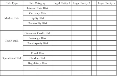
Finally, for reporting and steering purposes, an auditable output denoted “acknowledgment” (Ta-ble 4) matrix should be produced. Risk measures, losses and appetite should be reported against this matrix. Obviously, all the cells may not have to be completed depending on the activity or the legal entity. It is important pointing out that we do not focus on the residual risk yet, but on the inherent risk. This acknowledgment matrix provides a global vision of risk profile. Starting

with the residual risk may bias our vision by giving an incomplete risk profile4

.

From the previous analysis, a governance strategy may be highlighted. Based on banks capabil-ities i.e. the implementation of the strategy, the risk profile analysis and the measurement, the reporting and the communication, and the resulting actions, a five step implementation scheme arises:

1. measure the exposure and set the tolerances 2. set risk appetite

3. embed risk appetite 4. monitor and mitigate 5. revise.

Each and every metric can them be used to manage the couple risk-return, providing multiple management decision triggers. The following example illustrates various actions engendered by the breach of the thresholds.

1. An alert (e.g. KRI breaching a limit) triggers an escalation at the right level. The loss distributions should be stressed and the impact on the Expected Loss and the Tolerance

4

The residual risk may be defined as the difference between the inherent risk and the mitigating actions undertaken. The residual risk is discussed in this document but will be considered in companion papers as once the inherent risk has successfully been mitigated, the residual risks become the main risk of failures.

Group

Group

Departments / Divisions

Departments / Divisions

Business Units

Business Units

•Risk Tolerances per Category: Credit Risk, Market Risk, etc.

•Risk Limits per Category: Credit Risk, Market Risk, etc.

•KeyRisk Indicators

Given the company

capabilities and

resources, a risk

appetite process may be

implemented. However,

the process is not linear,

neither from the bottom

nor from the top, but a

mix of both. Achieving

this mix implementation

should lead to a

consistent risk

measurement, an

enhanced risk

framework (embedding)

and more accurate risk

management actions.

Given the company

capabilities and

resources, a risk

appetite process may be

implemented. However,

the process is not linear,

neither from the bottom

nor from the top, but a

mix of both. Achieving

this mix implementation

should lead to a

consistent risk

measurement, an

enhanced risk

framework (embedding)

and more accurate risk

management actions.

Business

Environment _{Risk Culture}

Stakeholders Objectives 17 Documents de Travail du Centre d'Economie de la Sorbonne - 2014.37