HAL Id: hal-02182030
https://hal.sorbonne-universite.fr/hal-02182030
Submitted on 12 Jul 2019HAL is a multi-disciplinary open access archive for the deposit and dissemination of sci-entific research documents, whether they are pub-lished or not. The documents may come from teaching and research institutions in France or abroad, or from public or private research centers.
L’archive ouverte pluridisciplinaire HAL, est destinée au dépôt et à la diffusion de documents scientifiques de niveau recherche, publiés ou non, émanant des établissements d’enseignement et de recherche français ou étrangers, des laboratoires publics ou privés.
damaged materials
Jia Li, Dominique Leguillon, Eric Martin, Xiao-Bing Zhang
To cite this version:
Jia Li, Dominique Leguillon, Eric Martin, Xiao-Bing Zhang. Numerical implementation of the coupled criterion for damaged materials. International Journal of Solids and Structures, Elsevier, 2019, 165, pp.93-103. �10.1016/j.ijsolstr.2019.01.025�. �hal-02182030�
Numerical implementation of the coupled criterion for damaged
materials
Jia Lia*, Dominique Leguillonb, Eric Martinc, Xiao-Bing Zhangd
a LSPM, CNRS UPR 3407, Institut Galilée, Université Sorbonne Paris Cité, Université Paris 13, F-93430 Villetaneuse, France
bInstitut Jean Le Rond d'Alembert, CNRS UMR 7190, Sorbonne Université, F-75005 Paris, France. c Laboratoire des Composites Thermo-Structuraux, CNRS UMR 5801, Université de Bordeaux,
F-33600, Pessac, France
d IUT d’allier, Institut Pascal, Université Clermont Auvergne, F-03100 Montluçon France
* Corresponding author.
ABSTRACT
In this work, we present a numerical model to deal with the fracture of damaged materials within the framework of the finite fracture mechanics (FFM). Continuum damage mechanics combined with the regularization techniques is first applied to determine the damage field. The transition from continuous damage field to discontinuous crack occurs when the coupled criterion (CC) is fulfilled. Special numerical algorithms were developed in crack path tracking and crack creation for the analysis of the entire failure process from damage development to crack creation. Both initiation and growth of one or multiple cracks can reasonably be simulated and efficiency and accuracy of the approach are illustrated through several numerical examples.
KEYWORDS:Finite Fracture Mechanics; Coupled criterion; Crack initiation and growth; Brittle or
quasi-brittle materials; Fracture; Damage 1.INTRODUCTION
Failure of quasi-brittle materials is characterized by the development of both diffused damage and macro-cracks. The final fracture in these materials is often preceded by the development of a process zone in which deformations localize, diffused damage such as micro-cracks or micro-cavities arises and accumulates. Fracture mechanics and continuum damage mechanics are the conventional tools used to tackle this class of problems although linear elastic fracture mechanics is not capable to describe the damage-induced nonlinear behavior of quasi-brittle materials. The most popular approach to remedy this shortcoming is to introduce the process zone concept into fracture mechanics analyses by using cohesive zone models (Barenblatt, 1962; Dugdale, 1960; Xu and Needleman, 1994). However, these models cannot
adequately capture diffuse degradation. Unlike the fracture mechanics approaches, another approach is based on continuum damage mechanics analyses, which can reasonably represent diffuse degradation (Lemaitre and Chaboche,1990) but it deteriorates in the final stage of failure due to spurious damage growth as the models are unable to represent discrete failure surfaces (Needleman and Tvergaard, 1984).
In quasi-brittle materials, and even in some brittle materials like ceramics, diffused damage before final fracture can be observed and cannot be neglected (Yousef et al., 2006). In this case, macro-cracks initiate and propagate in weakly damaged materials (Zimmermann et al., 2001). But neither pure fracture mechanics nor pure continuum damage mechanics is appropriate to describe correctly the entire failure process.
It is clear that the ideal approach is to combine the two descriptions to achieve a better characterization of failure as suggested in Janson and Hult (1977). To this end, efforts were made by coupling continuum damage to discontinuous models (Simone et al., 2003; Comi et al., 2007; Cazes et al., 2009). In general, it is assumed that when the damage parameter exceeds a predefined critical value, a traction-free crack or a cohesive crack is introduced in order to describe the final stages of failure. In most of these analyses, only crack growth problems were considered, while the crack initiation in damaged media has not been well assessed so far.
Recently, the coupled criterion (CC) was proposed as a finite fracture mechanics (FFM) approach to fulfil the need in fracture prediction of brittle materials. In studying the crack onset from the root of a sharp V-notch, Leguillon (2002) noticed that application of a single conventional fracture criterion, namely the Griffith energy criterion or the stress criterion, is not suitable and often leads to paradoxical predictions. It was concluded that when fracture occurs, both criteria have to be fulfilled simultaneously, even if one often predominates over the other. Application of this coupled criterion to crack onset predictions at a V-notch root shows remarkably satisfactory agreements with respect to experimental results. Afterward, the CC gets increasing popularity in fracture prediction of brittle or quasi-brittle materials. A large number of cases were studied by using this criterion (Nguyen et al. 2012; Mantic, 2009; Martin et al. 2010; Leguillon, 2011; Leguillon and Yosibash, 2003; Tran et al., 2012 among others).
The CC was further implemented into a finite element numerical model for simulating bi-dimensional cracking process in brittle materials (Li and Leguillon, 2018). Special numerical approaches were developed in drawing correctly the potential crack paths and to minimize the potential energy with respect to all predicted crack paths. This numerical model permits to consider more complex fracture problems in engineering applications (Li et al. 2018).
It is desirable to extend the CC to cracking prediction of damageable materials. Leguillon and Yosibash (2018) proposed such a coupling between the CC and a damage law but for a damage law exclusively dedicated to a V-notch root modeling. In the present work, we will
present a numerical scheme allowing applications of the CC to general 2D damage-fracture analyses. In this numerical scheme, continuous damage field is first evaluated by using the continuum damage mechanics theory enhanced by nonlocal regularization models. Then discontinuous cracks are created in damaged material according to the CC. This numerical scheme was implemented into a finite element code. A special algorithm was developed to simulate the crack nucleation and propagation. By carrying out numerical simulations on some well-studied structures, we illustrate the parameter identification of the damage-fracture model and the energy decomposition during the damage-fracture process. The ability and accuracy of the proposed model are also studied. It is shown that through the introduction of the CC in a nonlocal damage model, a more complete and realistic description of the entire failure process, from diffuse micro-cracking to macroscopic cracks, can be achieved.
2.MODEL DESCRIPTION
The failure of a quasi-brittle material is assumed to undergo damage before cracking. In general, damage and strain are localized in the most loaded area of the solid. Along the loci of the damage/strain concentration, cracks may appear and grow, leading to failure. Our main objective is to simulate numerically the entire damage-cracking process by using the CC.
2.1. Damage evolution laws
Among the numerous damage laws, the exponential law proposed by Mazars and Pijaudier-Cabot (1989) is widely applied to concretes. In this damage law, the damage scalar is defined as a function of the effective strain level:
(
)
(
)
0 0 0 0 0 if 1 1 exp ( ) if e c e e e d d < = − − + − − ≥ ε ε ε α α β ε ε ε ε ε (1) where α and β are two parameters of the model, ε0 is the threshold for damage initiationand dc is the maximal damage value before cracking. The equivalent strain εe in Eq. (1) can be
expressed through the modified von Mises definition (Vree et al., 1995):
(
)
(
)
(
)
2 1 1 2 2 1 1 1 12 2 1 2 1 2 1 ε ν ν ν − − = + + − − + e k k k I I J k (2)where ν is the Poisson ratio; k is the ratio of the tensile and compressive strength; I1 and
J2 are the first invariant of the strain tensor and the second invariant of the deviatoric part of the
strain tensor:
( )
(
) (
) (
)
1 2 2 2 2 1 2 2 3 3 1 trace 1 6 ε ε ε ε ε ε = = − + − + − I J ε (3) where ε1, ε2 and ε3 are the first, second and third principal stresses respectively. In practice,the nonlocal concept is often used in order to guarantee the mesh-independence of the damage model and to regularize the singularity-induced spurious damage localization. The damage driving quantity in this model, namely the nonlocal equivalent strain εe, can be calculated by using either the integral or the differential approaches. The integral approach calculates a weighted average of the equivalent strain (Pijaudier-Cabot and Bazant, 1997):
(
) ( )
e e V x y y dy =∫
− ε ϕ ε (4) where ϕ(
x−y)
is a weighting function which describes the non-local interaction. Mathematically, the normalization condition( )
1V
y dy=
∫
ϕ is required. Hereafter we adopt the following weighting function in : 2( )
2 2 2 3 1 if 2 4 4 0 if 2 r r l r l l r l − ≤ = > ϕ π (5)where l is the length scale parameter and 2l represents the radius of the nonlocal influence area. The differential approach consists in resolving a modified Helmholtz equation with the equivalent strain εe as the source term (Peerlings et al., 2001):
2
εe− ∆ =l εe εe
(6) which, together with the homogeneous natural boundary condition
. 0 ε ∇ en=
(7) complete the coupled system of equations. It was shown that these two approaches are mathematically equivalent (Peerlings et al., 2001). The selection of one or the other approach depends on the type of the problem to be solved. Generally speaking, the differential approach is suitable for homogeneous materials. When the material embeds several phases, the integral
approach is more appropriate as the nonlocal equivalent strain can easily be evaluated separately in each phase.
Once the nonlocal equivalent strain field is obtained, the damage field can be evaluated by substituting εe by εein Eq. (1).
The constitutive equation is simply written as:
(
1)
: = − dσ D ε (8)
Another damage law (Geers et al. 1998) may be more suitable for brittle materials in which cracking occurs in weak damage conditions:
0 0 1 1 0 1 0 1 0 if 1 if if < − = − ≥ ≥ − > e e c e e c e d d d β α ε ε ε ε ε ε ε ε ε ε ε ε ε (9) In this damage law, ε0 is the threshold for damage initiation andε represents the value of 1
e
ε for which damage reaches its limit value. The parameters of the model α and β influence the slope and the shape of the softening curve, respectively. In practice, the equivalent strain εe should be replaced by its nonlocal counter-part εein order to guarantee the mesh-independence of the damage model.
2.2. The coupled criterion for damaged materials
Within a plane elasticity framework, Leguillon (2002) states that a new crack is created if and only if both the stress and energy conditions are verified, i.e., the stress criterion is satisfied at all points along the presupposed crack path, and the energy balance is fulfilled with the corresponding crack path. These two conditions form the so-called coupled criterion (CC). It was widely presented in the literature (see the review paper by Weissgraeber et al., 2016), thus hereafter we very briefly recall the bases and highlight the changes to bring when damage develops prior to cracking.
Consider the initial state of a loaded solid just before cracking and the final state of the same solid after the creation of a new crack or the growth of an existing one. The incremental energy balance between these two states writes:
( )
,( )
,(
,)
0where f, u and ε represent the external force, the displacement field and the strain field respectively. ∆Uext and ∆Ustrain are the incremental potential energy of external force and the incremental strain energy of the solid. ∆Ucrackis the incremental energy consumed by the crack growth. ∆Ukinetic includes the other energy dissipated during the cracking process, essentially the kinetic energy. ∆S is the surface of the crack increment. It is clear that ∆Ustrain depends not only on the strain state but also on the damage state of the solid.
The energy consumed by the crack growth leads to the definition of the critical fracture energy rate, as follows:
crack c U G S ∆ = ∆ (11)
By defining the incremental energy release rate Gincas follows inc Uext Ustrain
G
S S
∆ + ∆ ∆Π
= − = −
∆ ∆ (12)
where ∆Uext+ ∆Ustrain = ∆Π is the variation of the total potential energy. The energy condition states that the crack creation occurs when
inc c
G ≥G
(13)
In general, the kinetic and other dissipated energy is not nil. Its variation can be calculated according to equations (10-12):
(
inc)
kinetic c U G G S ∆ = − ∆ (14) This energy criterion is not sufficient since it depends on the newly created surface ∆S (up to now unknown). In order to remedy this shortcoming, the CC suggests to add the stress condition. The general form of the stress criterion writes:σe ≥σc all over the surface ΔS prior to fracture (15) where σe and σ are respectively the nominal driving stress and the ultimate stress for a c undamaged material. Solving the two inequalities makes it possible to determine ΔS and then the failure load.
For damaged materials, this stress criterion cannot be directly applied due to the stress softening. In this case, the nominal stress has to be replaced by its effective value σe
(
1−d)
. Inthese conditions Eqn. (15) can be rewritten:
e (1 d) c
σ ≥ − σ
This implies that the damage, which softens the material behavior, also reduces its tensile strength in the same proportion. Under these conditions, the “local” (or “damaged”) Irwin length becomes: local c Irwin Irwin 2 c (1 ) 1 EG l l d σ d = = − − (17)
where E, Gc, σc and lIrwin are data of the sound material and d is the damage parameter. For a pure
mode-I crack, the Irwin length lIrwin represents the distance between the crack tip and the point
where the circumferential tensile stress is σc. According to the CC, the crack jump length is
proportional to the Irwin length, therefore the crack jump is likely to be longer in the damaged area than in the sound material. However, caution should be taken in this statement because the damage field d is not uniform in the solid.
Moreover, this stress-based criterion can equivalently be replaced by the strain-based criterion, namely:
d ≤ c
ε ε (18)
where ε and d εc are respectively the driving strain and its critical value at fracture. For example, if the first principal stress is taken as the driving stress in brittle or quasi-brittle materials, the stress criterion (16) in damageable isotropic material becomes, in a 3D setting:
(
)
1 1 12 2 3 1 1 effective c c E E d = = + + ≥ = − − σ σ ε ν ε ε σ ε ν (19)Therefore, the strain criterion (18) is applicable by taking
(
)
1 2 3 2 1 1 d = − + + ε ε ν ε ε ν (20)Thus the strain-based fracture criterion (18) can directly be applied.
One of the main advantages of the CC is its ability to predict both the crack initiation and crack growth. Its numerical implementation is easy by adopting efficient crack path tracking technics.
According to the above analyses, the energy decomposition during the crack creation can easily be performed by using the following formulas:
Total strain energy:
(
)
0 :
strain
U d d
Ω
=
∫ ∫
εσ ε Ω (21)Elastic strain energy: 1 2 elastic
U d
Ω
Total dissipated energy: Udissip =Ustrain −Uelastic (23) Increment of the fracture energy: ∆Ucrack =Gc∆ S (24) Damage energy : Udamage =Udissip−Ucrack −Ukinetic (25)
In Eq. (25), the total fracture energy Ucrack and the total kinetic energy Ukinetic can be calculated by accumulation according to (24) and (14), respectively.
2.3. Crack tracking
The coupled criterion cannot be correctly applied without knowledge on the crack path. In Li and Leguillon (2018), a crack tracking method has been proposed for 2D linear elastic solids. Hereafter we just summarize briefly this technique, its detailed description can be found in the original paper.
The crack path is assumed to be perpendicular to the maximal principal stress. The crack tracking procedure is divided into 2 steps.
The first step is to find all the zones in which the driving strain εd is larger than its critical value by using a so-called watershed flooding technique, whose description was given in Li and Leguillon (2018). Such zones contain a local maximum of ε from which a potential crack can d be created.
The second step consists in finding the actual crack path among all potential crack paths in each zone where εd ≥εc. Here we assume that the newly created crack is perpendicular to the first principal stress. This criterion permits to draw a principal stress trajectory from each local maximum of εd. Simultaneously, the length of the crack path is calculated.
In order to determine which potential crack path becomes a real crack, we active successively all the potential cracks (index i) paths and calculate their incremental energy release rate Giinc. If the maximum of Giincfulfills the Griffith criterion maxGiinc ≥Gc, a real crack will be created accordingly.
For the creation of new cracks, different approaches exist in the finite element method. Herein the element elimination technique (Li et al., 2015) is used for the sake of simplicity. We find all elements in interception with the predicted crack paths, and then remove them from the finite element model. According to the theoretical and numerical studies of Pandolfi and Ortiz
(2012), this element erosion method converges to the Griffith fracture with infinitesimal mesh sizes and does not exhibit spurious mesh dependencies.
The coupled criterion for damaged materials together with the crack tracking method were implemented into a dedicated finite element code in order to perform bi-dimensional simulations.
2.4. Overall algorithm
The external loads are applied incrementally by imposing displacements on the boundaries of the solid up to a prefixed level. A full Newton–Raphson procedure has been used to trace the response in the non-linear regime. Hereafter we describe briefly the global algorithm used in the finite element implementation of the damage-fracture model in the form of pseudo-code:
Algorithm
Require: Displacement, stress, strain and damage fields at time tn
1. Set time to tn+1, update the external loads;
2. Equilibrate nonlinear field of the damageable elastic solid and calculate Π0;
3. Find N zones in which εd ≤εc; 4. for each zone i=1 to N do
5. Determine the crack path, evaluate the crack length increment ∆li ; 6. Activate this crack, equilibrate nonlinear field and calculate Πi;
7. Calculate Giinc = − Π − Π
(
i 0)
∆li; 8. Deactivate this crack;9. end for
10. Find Gmaxinc =max
( )
Giinc ; 11. if Gmaxinc ≥Gcthen12. Create the corresponding crack, go to 2; 13. else
14. go to 1; 15. end if
Note that the above-described algorithm assumes that the damage evolution and the crack creation are sequential events in numerical simulations. Equilibrium has to be achieved after
damage increment and crack creation in each loading step. Therefore, numerical implementation of the CC is independent of choice of the damage law and can always be applied if convergence can be attained in damage calculation.
3.MODEL CALIBRATION AND NUMERICAL EXAMPLES
In the following, the CC based damage-fracture model is applied to resolve some fracture problems in brittle or quasi-brittle materials. The simulation results are compared to well-known solutions in order to verify the performance of the proposed model. In the following, the 3-node triangle elements are used.
3.1 crack propagation in a PMMA plate
PMMA is generally considered as a brittle material. Therefore, the damage evolution is often neglected in its fracture modeling. However, Ravi-Chandar and Yang (1997) showed that diffused damage can develop in the form of micro-cracks ahead the main crack tip. Therefore, introducing the damage phenomenon in the crack growth modeling may physically be more realistic.
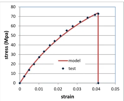
In numerical simulations, Eq. (9) is selected as the damage evolution law. The values of the elasticity constants are Young’s modulus E = 3000 MPa and Poisson’s ratio ν = 0.28. By fitting the constitutive law (Eqs. 8-9 in 1D) with the stress-strain curve of previous tensile tests (Li and Zhang, 2006), we identify the material parameters: ε0=0.005; ε1=0.5; α =5; β =0.1; d =0.9. The c
critical strain is set to εc =0.041, corresponding to an ultimate stress σ ≈c 73 MPa . The comparison between the theoretical stress-strain curve and the experimental data is shown in Figure 1. It is worth mentioning that the viscosity of the material is not considered in this model and the only source of non-linearity is assumed to be the damage effect.
Figure 1. Parameter identification by fitting the model to the experimental data (Li and Zhang, 2006).
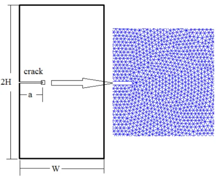
A PMMA plate of dimension 2H × 2W containing a central crack of length 2a is subjected to a mode-I tensile loading, H = 5 mm is the half height and W = 5 mm is the half width of the plate. The apparent critical energy release rate of PMMA is about Gcapparent = 0.29 MPa mm (Li and Zhang, 2006). This energy dissipation value includes both the damage-induced dissipation and the fracture energy. Therefore, the critical energy release rate for the only crack growth
crack c
G should be smaller than this value. Using numerical results, the calibrated value is Gccrack = 0.13 MPa mm for the main crack propagation. The difference between Gcapparent and Gccrackresults from the dissipation due to damage.
0 10 20 30 40 50 60 70 80 0 0.01 0.02 0.03 0.04 0.05 st re ss (Mp a) strain model test
Figure 2. Plate with a central crack and the near tip mesh (half structure is presented due to the symmetry)
The differential non-local model (6) is used to evaluate the non-local effective strain with the length scale parameter l = 0.01 mm and we evaluate the critical remote loads for crack growth with an initial central crack of different sizes, namely a/W = 0, 0.03, 0.04, 0.06, 0.08, 0.1, 0.2, 0.3, 0.4 and 0.5, here a = 0 corresponds to the plate without crack. In order to investigate the influence of the mesh size, different element sizes near the crack tip and along the crack path are used in the simulations, d = 0.003, 0.005 and 0.01mm, where d is the average edge length of the triangular elements. A uniaxial tension along the normal direction to the crack was applied at the ends of the plate prescribing incrementally increasing displacements. The remote load at fracture is defined as the peak value of the load-displacement curve.
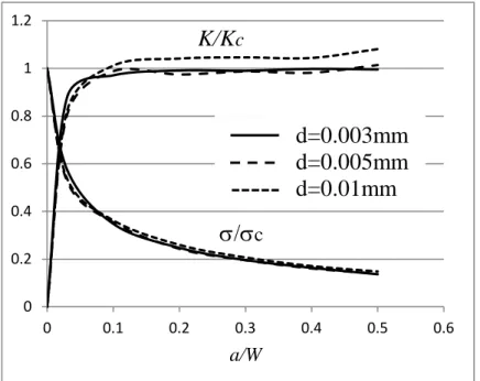
The predicted critical remote stress σ∞ at crack propagation is now used to calculate the stress intensity factor K with the help of the handbook of stress intensity factors (Sih, 1973). By comparing the stress intensity factors to the critical valueKcapparent = EGcapparent , we can evaluate the accuracy of the method for crack growth prediction. The values of K Kcapparentat crack growth for different crack lengths are shown in Figure 2, where the ratios σ σ∞ care also plotted.
From this figure, we can observe that for sufficiently long cracks (a/W > 0.05), the normalized stress intensity factorK Kcapparent ≈ . Therefore, the stress intensity factors at fracture 1 evaluated using the CC equal correctly the measured material toughness. This simulation also shows that the calibration of such a damage-fracture model is feasible even though it is more complicated than that for a pure fracture model or a pure damage model.
We can also remark that the proposed model is weakly mesh-sensitive when sufficiently refined meshes are used. The element size with d = 0.01mm represents quite a coarse mesh, the numerical calculations with this mesh density induce errors smaller than 10% on K Kcapparent. The calculations with finer meshes, e.g. d = 0.003mm and 0.005mm, provide very close values for remote loads at fracture. The predicted crack path should contain sufficient number of elements in order to guarantee a good accuracy on the stress and energy calculations. In the present example, the results with d = 0.003mm are shown.
Figure 2. Normalized stress intensity factor K Kcapparentand normalized remote stress σ σ∞ c at failure as a function of the normalized semi-crack length a/W for mode-I loaded cracks.
Next, we consider the energy evolution during the propagation of a crack with a = 1 mm. Under displacement-imposed loading, the damage distributions of the early stage crack growth, calculated with two different mesh densities d=0.003mm and d=0.01mm, are shown in Figure 3.
0 0.2 0.4 0.6 0.8 1 1.2 0 0.1 0.2 0.3 0.4 0.5 0.6 a/W
K/K
cσ/σ
cd=0.003mm
d=0.005mm
d=0.01mm
As expected, a thin damage band is created around the crack path. We can also remark that the damage distribution obtained with a quite coarse mesh, even though less regular, is close to that obtained with a refined mesh.
In order to analyze the energy consumed during the crack growth, we plot the evolution of the different dissipated energies as a function of crack extension in Figure 4. This figure shows that, under displacement controlled loading, the total strain energy attains a critical value when the crack begins to grow, then increases as the crack go on growing and finally remains unchanged regardless of the crack growth. The elastic strain energy decreases while the total energy dissipation increases as the crack grows. The latter is the sum of the energies consumed in new crack creation, in diffused damage and in waves propagation (kinetic energyUkinetic, see Eq.10) respectively. Pracically, as it is difficult to separate the energies dissipated by damage and by crack growth in a mechanical test, the critical energy release rate is experimentally measured by means of their sum according to Gcapparent = ∆
(
Udamage+ ∆Ucrack)
∆ . The energy S decomposition method used in the present work can help to identify the true energy release rate dedicated exclusively to the crack formation.Figure 5 illustrates the variation of the apparent energy release rate as function of the crack propagation. We observe a globally increasing trend of Gcapparentas crack grows. This trend was largely reported in the literature and named as the R-curve effect (Heyer, 1973). According to the present results, the increase of the apparent energy release rate is essentially due to the increase of the diffused damage area ahead the crack tip, as shown in Figure 3.
Figure 3 brings into evidence the intermittent mechanism governing the crack growth. It can be explained as follows: (i) in a first step damage develops near the crack tip where there is a strong stress concentration, (ii) in a second step, according to the CC, the crack jumps a given length, (iii) and then it grows toward a less damaged zone with higher Young’s modulus (Eqn. (8)) and tensile strength (Eqn. (16)). Then, again damage develops at the new crack tip and so on. It seems that this mechanism tends to reach a steady state as can be observed in Figure 3 on the right.
This damage-cracking sequence was supported by previous experiments (Ravi-Chandar and Balzano, 1988; Ravi-Chandar and Yang, 1997). Their clearly showed that in some amorphous materials such as the PMMA, crack propagation occurs by a mechanism of nucleation, growth and coalescence of microcracks. The microcracks are first formed ahead of the main crack, then their number and size increase and they finally coalesce with the main crack. This damage-cracking process results in a periodic morphology of the crack surface, especially for a fast-growing crack. As pointed in Ravi-Chandar and Yang (1997), the size of the fracture process zone increases as the stress intensity factor increases. This experimental observation agrees with the sequential damage-craking scenario shown here.
(a) d=0.003mm (b) d=0.01mm
Figure 3. Damage distributions around the crack path obtained with two mesh sizes for a PMMA plate with a central crack subjected to traction
Figure 4. Energy decomposition during the crack growth
Figure 5. Variation of apparent energy release rate as function of crack growth
3.2: Crack initiation in a PMMA plate
The CC can be used also for crack initiation prediction. To illustrate this capacity, we consider a rectangular PMMA plate subjected to a uniaxial tensile loading. In order to ensure that the fracture occurs in the central part of the plate, its width is slightly reduced in the middle, as
0 0.5 1 1.5 2 2.5 3 3.5 4 0 0.5 1 1.5 en er gy (N .mm)
crack growth length (mm) U strain U elastic U dissip U crack U damage U kinetic y = 0.0199x + 0.2897 0 0.05 0.1 0.15 0.2 0.25 0.3 0.35 0.4 0 0.5 1 1.5 2 ap pa ren t en er gy rel ea se ra te (M Pa .mm)
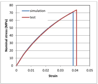
shown in Figure 6. The same mechanical parameters have been used as in the previous example. In Figure 7, we plot the comparison of the remote stress-strain curves issued from numerical simulations and experimental results reported in Li and Zhang (2006). The non-linear behavior of PMMA is approached by the emergence and development of damage in the material. The remote stress at fracture found from the simulation is slightly smaller than that of the mechanical test due to the slight geometrical reduction in the middle in order to trigger a stress concentration. Figure 6 shows the crack path and the damage distribution throughout the plate. A similar mechanism of intermittency (Section 3.1) seems to develop in this case but with different features. Damage develops first, more or less homogeneously as can be seen on Figure 6a, the necking being small enough to avoid strong stress concentrations. As a consequence, prior to any crack appearance the material is already damaged with d ≈ 0.4, then, according to (17), the Irwin length is larger and the crack jump at onset is larger as well. The crack nucleates in the middle of the left edge where there is still a small stress concentration. As previously described, the crack grows toward a less damaged zone where Young’s modulus and tensile strength are larger and then stops. Following, damage increases at the crack tip before a new crack jump. Comparing Figures 3 and 6, it is clear that the pseudo-periodicity of the intermittency is far larger in the second case due to the uniformly damaged material prior to the appearance of a crack. Note that the color scales differ on the left and right part of Figure 6 in order to highlight the nearly homogeneous damage distribution prior to the crack onset.
It is also necessary to note that the inertial effects are not taken into account in the present analysis, even though the fracture process is very rapid (Li and Zhang, 2006).
Figure 6. (a) Damage distribution before cracking; (b) Damage distribution and crack path at final failure in the PMMA plate
Crack initiation
Figure 7. Remote stress-strain curves issued from simulation and experiment
3.3. Crack initiation and growth in concrete beams
It is commonly admitted that concrete is a quasi-brittle material. Very high level damage can be reached before crack creation or crack growth. Therefore, neglecting the diffused damage in fracture process or neglecting the cracking in damage evolution will both lead to unphysical description of the concrete failure. The CC combined with damage modeling permits to remove this shortcoming.
In order to illustrate the capacity of the present model in dealing with the fracture behavior of concrete structures, we simulated some experimental results reported in the literature (Kozlowski et al., 2015). Foamed concrete beams with notches were tested under 3-point bending. Geometry and loading conditions are illustrated in Figure 8. Four different concrete mixtures resulting in varying densities were used in the experiments (Kozlowski et al., 2015).
0 10 20 30 40 50 60 70 80 0 0.01 0.02 0.03 0.04 0.05 No mi na l s tre ss (MP a) Strain simulation test
Figure 8. Geometry and loads of a 3-point concrete beam
In numerical simulations, the damage evolution law Eq. (1), together with the nonlocal scheme Eq. (6) was used. The mechanical parameters used are listed in Table 1. The principal mechanical characteristics, namely ε0 and Gc were estimated according to the data provided by
Kozlowski et al. (2015). Here we fixed ν = 0.2, α = 1, εc = 5ε0 , dc = 1, k =10 and l = 2 mm. The
others parameters, namely E and β, were adjusted according to the experimental load-deflection curves.
Table 1.Material parameters for foamed concretes
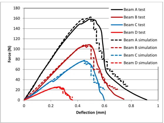
The comparison between the simulated and measured global load-deflection responses are plotted in Figure 9. These curves show that the present damage-fracture model describes well the quasi-brittle fracture behavior of the different foamed concrete beams.
E(Mpa) ν α β ε0 εc Gc(MPa mm) dc k l(mm) Beam A 950 0.2 1 220 0.001 0.005 0.0060 1 10 2 Beam B 600 0..2 1 380 0.00125 0.00625 0.0018 1 10 2 Beam C 450 0.2 1 450 0.00123 0.00615 0.0009 1 10 2 Beam D 270 0.2 1 600 0.00064 0.0032 0.0004 1 10 2 800mm 100mm 42mm 840mm 3mm P
Figure 9. Comparison between simulation and experimental responses of 3-point loaded foamed beams
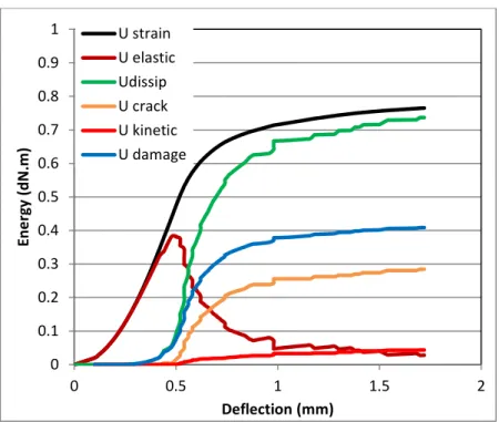
Figure 10 illustrates the decomposition of the strain energy as a function of the deflection of beam A. This figure shows the evolution of the different parts of energy consumed during the damage-fracture process. It indicates especially the important amount of energy dissipated by the diffused damage, which is a noticeable feature of quasi-brittle materials. Here again, the energy decomposition method can help to separate the fracture energy from the damage energy in experimental tests. 0 20 40 60 80 100 120 140 160 180 0 0.2 0.4 0.6 0.8 1 Fo rc e ( N) Deflection (mm) Beam A test Beam B test Beam C test Beam D test Beam A simulation Beam B simulation Beam C simulation Beam D simulation
Figure 10. Energy decomposition as function of deflection (Beam A)
In order to compare the present model with the pure damage model, we also carried out simulations by using the damage model alone for beam A. As pointed in Simone et al. (2003), the damage laws used in the damage-fracture model is necessarily different from that used in the pure damage model and requires a re-assessment. The parameters in the pure damage model are ε0 = 0.0001 and β = 280, the other parameters being identical to those used in the
damage-fracture model. In Figure 11, we display the load-deflection responses provided by the two models and compared with the experimental results. The comparison shows that both models are able to describe the global behavior of the beam.
In Figure 12, we present the damage zones obtained by using these two models in beam A. As expected, the damage develops along the middle ligament of the beam. Nevertheless a real crack is created in the damage-fracture model with a smaller damage zone and lower damage level compared to the pure damage model. It is clear that the failure description of the damage-fracture model avoids any over estimation of the damaged zone.
0 0.1 0.2 0.3 0.4 0.5 0.6 0.7 0.8 0.9 1 0 0.5 1 1.5 2 En erg y ( dN .m) Deflection (mm) U strain U elastic Udissip U crack U kinetic U damage
Figure 11. Load-deflection responses obtained by using the pure damage model and damage-fracture model compared with the experimental result
(a) (b)
Figure 12. (a) Damage distribution and crack path in damage-fracture model, (b) damage distribution in pure damage model
3.4. Crack path tracking
In order to illustrate the ability of the proposed model in tracking the crack path, we consider a notched concrete beam under mixed mode loading, according to Galvez et al. (1998) tests. The geometry and loading conditions of one of these beams are displayed in Figure 13. Stable tests were achieved by applying load through a servo-controlled testing machine running
0 20 40 60 80 100 120 140 160 180 0 0.2 0.4 0.6 0.8 1 Lo ad (N ) Deflection (mm)
Beam A damage only Beam A damage+fracture Beam A test
under CMOD (crack mouth opening displacement) control. The principal aim of numerical simulations on these experiments is to examine the crack path tracking ability of the present damage-fracture model by comparing the numerical and experimental results. The material parameters used in the simulations are (partially) given in [34], namely E = 38 GPa, ν = 0.2; εc =
0.0000789, Gc = 0.02 MPa mm. Here the value of the critical energy release rate is smaller than
the apparent value 𝐺𝐺𝑐𝑐𝑎𝑎𝑎𝑎𝑎𝑎𝑎𝑎𝑎𝑎𝑎𝑎𝑎𝑎𝑎𝑎= 0.069 MPa.mm given in Galvez et al. (1998), which includes the damage-dissipated energy. The other damage parameters used in Eq. 1 and Eq. 6 are: α = 0.92; β = 300; dc = 0.8, l = 2 mm.
Figure 13. Geometry and boundary conditions of a mixed-mode-loaded beam
In Figure 14, we compare the simulated crack path with the experimental records. The crack path obtained by using the classical maximal tensile stress (MTS) criterion of LEFM (Galvez, 1998) is also plotted for comparison. This figure shows that the crack path predicted by the current model agrees well with the experimental observation and gives even a better fit than the classical LEFM theory.
675mm
375mm 37,5mm
75mm
150mm 187,5mm
Figure 14. Crack paths obtained by using the damage-fracture model and the MTS criterion compared with the experiment records
3.5. Multi-cracking simulation
The present numerical approach permits to handle initiation and growth of several cracks and especially the cracking process in heterogeneous media. In fact, all the possible new crack loci are examined by applying the CC and the best combination of them that makes the total potential energy minimal is selected as the next crack extensions. In the following, we illustrate this feature by considering a composite plate made of three phases: matrix, inclusions and interphase. The dimension of the composite plate is 50 × 50 mm². The circular inclusions are randomly distributed in the plate and their diameter is varying from 4 to 10 mm. The interphase between matrix and inclusion is represented by a thin layer of material with a thickness of 0.3 mm. The inclusions are assumed to be undamageable and unbreakable. The volume ratio of the inclusion+interphase is 55%. Eq. (1) is used as the damage evolution law for matrix and interphase. The non-local effective strains are calculated in each phase separately. It is therefore more convenient to apply the integral non-local approach, i.e. Eq. (4). The mechanical properties of the constituents are listed in Table 2.
Table 2. Material parameters for composite plate with inclusions
We simulate the damage and cracking process of the heterogeneous plate under uniaxial tension. Figure 15 shows the global strain-stress response. Figure 16 presents the crack patterns at the load peak and at the final fracture stage. As the interphase between matrix and inclusions is the weakest part of the composite, multiple crack initiations occur first along the interphase. Then these cracks propagate in the matrix and coalesce to form predominant macro-cracks. This scenario describes faithfully the fracture mechanism in concrete or in some composites in which the interface exhibits a weaker mechanical resistance.
Figure 15. Simulated stress-strain response of a composite plate under tensile loading
0 1 2 3 4 5 6 7 0 0.0005 0.001 0.0015 St re ss (Mp a) Strain E (MPa) ν α β ε0 εc Gc (MPa mm) dc K l2 (mm2) Matrix 950 0.2 1 250 0.001 0.005 0.006 1 10 2 inclusions 950 0.2 - - - ∞ ∞ - - - interphase 950 0.2 1 250 0.0003 0.0017 0.002 1 10 2
(a) (b)
(a) (b)
Figure 16. Damage distributions and crack patterns in the composite plate. (a)(b): at load peak (c)(d): at final fracture
4.CONCLUDING REMARKS
In this paper, a numerical model for fracture of damaged materials has been proposed on the basis of the coupled criterion and implemented into a finite element code for simulating a two-dimensional damage-fracture process. The reliability and accuracy of the model have been illustrated by numerous examples for which solutions are well-known or well-studied in the
literature. This numerical model presents several advantages, including the possibility of describing the entire damage-fracture process, predicting both crack initiation and crack growth and considering multi-cracking problems. The coupled criterion is conceptually simple and physically reasonable. This work shows that it can also be applied to fracture prediction of damaged materials. Its numerical implementation opens a new way to describe the cracking process in solids. We believe that many other complex problems in fracture evaluations can be treated by developing more operational numerical tools.
Reference
Barenblatt, G.I., 1962. The mathematical theory of equilibrium cracks in brittle fracture, Adv. Appl. Mech. 7, 55-129.
Cazes, F., Simatos, A., Coret, M., Combescure, A., 2009. A cohesive zone model which is energetically equivalent to a gradient-enhanced coupled damage-plasticity model, Europ. J. Mech. A/ Solids, 976-989
Comi, C., Mariani, S., Perego, U., 2007. An extended FE strategy for transition from continuum damage to mode I cohesive crack propagation, Int. J. Numer. Anal. Methods Geomech. 31, 213–238 Dugdale, D., 1960. Yielding of steel sheets containing slits, J. Mech.Phys.Solids, 8, 100-104.
Galvez, J.C., Elices, M., Guinea, G.V.,Planas, J., 1998. Mixed mode fracture of concrete under proportional and nonproportional loading, Int. J. Fract., 94, 267–284.
Geers, M., de Borst, R., Brekelmans, W., Peerlings, R., 1998. Strain-based transient–gradient damage model for failure analyses, Comput. Methods Appl. Mech. Engrg. 160, 133–153.
Heyer, R.H., 1973. Crack growth resistance curves (R-curves)- literature review, in Fracture toughness evaluation by R-curve methods, ASTM STP 527, 3-16
Janson, J., Hult, J., 1977. Fracture mechanics and damage mechanics–a combined approach, J. Méch. Appl. 1, 69–83.
Kozłowski, M., Kadela, M., Kukiełk, A., 2015. Fracture energy of foamed concrete based on three-point bending test on notched beams, Procedia Engineering 108, 349 – 354
Leguillon, D. Yosibash, Z., 2003. Crack onset at a V-notch. Influence of the notch tip radius, Int. J. Fract. 122, 1-21.
Leguillon, D., 2002. Strength or toughness? A criterion for crack onset at a notch. Europ.J. Mech. A/Solids 21, 61-72.
Leguillon, D., 2011. Determination of the length of a short crack at a v-notch from a full field measurement, Int. J. Solids Struct., 48, 884–892.
Leguillon, D., Yosibash, Z., 2017. Failure initiation at V-notch tips in quasi-brittle materials. Int. J. Solids Structures 122-123, 1-13.
Lemaitre J., Chaboche J.L., 1990. Mechanics of solid materials. Combridge: Combridge University Press. Li, J., Leguillon, D., 2018. Finite element implementation of the coupled criterion for numerical
simulations of crack initiation and propagation in brittle or quasi-brittle materials, Theor. Appl. Fract. Mech. 93, 105-115
Li, J., Martin, E., Leguillon, D., Dupin, C., 2018. A finite fracture model for the analysis of multi-cracking in woven ceramic matrix composites. Composites Part B, 139, 75–83.
Li, J., Song, F., Jiang, C., 2015. A non-local approach to crack process modeling in ceramic materials subjected to thermal shock, Eng. Fract. Mech. 133, 85–98.
Li, J., Zhang, X.B., 2006. A criterion study for non-singular stress concentrations in brittle or quasibrittle materials, Engng. Fract. Mech. 74, 505-523.
Mantič, V., 2009. Interface crack onset at a circular cylindrical inclusion under a remote transverse tension. Application of a coupled stress and energy criterion, Int. J. Solids Struct. 46, 287–1304
Martin, E., Leguillon, D., Carrère, N., 2010. A twofold strength and toughness criterion for the onset of free-edge shear delamination in angle-ply laminates, Int. J. Solids Struct. 47, 1297–1305.
Mazars, J., Pijaudier-Cabot, G., 1989. Continuum damage theory––application to concrete, J. Engrg. Mech. 115, 345–365.
Needleman, A., Tvergaard, V., 1984. Finite element analysis of localization in plasticity. In: J.T. Oden and G.F. Carey (Eds.), Finite elements, Special problems in solid mechanics, Prentice-Hall, New Jersey, 94–157.
Nguyen, L.M., Leguillon, D., Gillia, O., Riviere, E., 2012. Bond failure of a SiC/SiC brazed assembly, Mech. Mater.50, 1–8.
Pandolfi, A., Ortiz, M., 2012. An eigenerosion approach to brittle fracture, Int. J. Numer. Methods Eng., 92, 694–714.
Peerlings, R., Geers, M., de Borst, R., Brekelmans, W., 2001. A critical comparison of non-local and gradient-enhanced softing continua. Int. J. Solids Struct.,38, 7723–46.
Pijaudier-Cabot, G., Bazant, Z.P., 1987. Nonlocal damage theory. J Engng Mech, ASCE,113, 1512–1533. Ravi-Chandar, K., Balzano, M., 1988. On the mechanics and mechanisms of crack growth in
polymeric materials, Eng. Fract. Mech., 30, 713-727.
Ravi-Chandar, K., Yang, B., 1997. On the role of microcracks in the dynamic fracture of brittle materials, J. Mech. Phys. Solids, 45, 535–63
Sih, G., 1973. Handbook of stress-intensity factors, Lehigh University.
Simone, A., Wells, G.N., Sluys, J., 2003. From continuous to discontinuous failure in a gradient-enhanced continuum damage model, Comput. Methods Appl. Mech. Engrg. 192, 4581–4607
Tran, V.X., Leguillon, D., Krishnan, A., Xu, L.R., 2012. Interface crack initiation at V-notches along adhesive bonding in weakly bonded polymers subjected to mixed-mode loading, Int. J. Fract. 176, 65-79.
Weissgraeber, P., Leguillon, D., Becker, W., 2016. A review of Finite Fracture Mechanics: Crack initiation at singular and non-singular stress-raisers. Archive Appl. Mech. 86, 375-401.
Xu, X.P., Needleman, A., 1994. Numerical Simulation of Fast Crack Growth in Brittle Solids. J. Mech. Phys. Solids 42, 1397-1434.
Yousef, S.G., Rodel, J., Fuller Jr., E. R., Zimmermann, A., El-Dasher, B. S., 2005. Microcrack Evolution in Alumina Ceramics: Experiment and Simulation, J. Am. Ceram. Soc., 88, 2809–2816. Zimmermann, A., Carter, W.C., Fuller Jr., E.R., 2001. Damage evolution during microcracking of brittle