HAL Id: hal-01462575
https://hal.archives-ouvertes.fr/hal-01462575
Submitted on 6 Jun 2020
HAL is a multi-disciplinary open access archive for the deposit and dissemination of sci-entific research documents, whether they are pub-lished or not. The documents may come from teaching and research institutions in France or abroad, or from public or private research centers.
L’archive ouverte pluridisciplinaire HAL, est destinée au dépôt et à la diffusion de documents scientifiques de niveau recherche, publiés ou non, émanant des établissements d’enseignement et de recherche français ou étrangers, des laboratoires publics ou privés.
Estimating price elasticities of food trade functions: how
relevant is the CES based gravity approach?
Alexandre Gohin, Fabienne Femenia
To cite this version:
Alexandre Gohin, Fabienne Femenia. Estimating price elasticities of food trade functions: how relevant is the CES based gravity approach?. [University works] auto-saisine. 2007, 35 p. �hal-01462575�
Institut National de la recherche Agronomique
Unité d'Economie et Sociologie Rurales
4 Allée Adolphe Bobierre, CS 61103 F 35011 Rennes Cedex
Tél. (33) 02 23 48 53 82/53 88 - Fax (33) 02 23 48 53 80 http://www.rennes.inra.fr/economie/index.htm
Estimating price elasticities of food trade functions:
How relevant is the gravity approach?
Fabienne FEMENIA et Alexandre GOHIN
March 2007
Estimating price elasticities of food trade functions:
How relevant is the gravity approach?
Fabienne FEMENIA INRA – Unité ESR Rennes
Alexandre GOHIN
INRA – Unité ESR Rennes, CEPII
The authors acknowledge financial support by the “Agricultural Trade Agreements (TRADEAG)” project, funded by the European Commission, DG Research (Specific Targeted Research Project, Contract no. 513666). The authors thank A. Carpentier and participants to the winter 2006 IATRC meeting for their valuable comments. The authors are solely responsible for the contents of this article.
Corresponding address Alexandre GOHIN INRA – Unité ESR
4 Allée Bobierre, CS 61103 35011 Rennes Cedex, France
Estimating price elasticities of food trade functions: How relevant is the gravity approach?
Abstract
The main objective of the article is related to the long standing issue of the econometric estimation of price elasticity of food trade functions. We investigate the relevance of the prominent gravity approach. This approach is based on the assumptions of symmetric, monotone, homothetic, CES preferences. We test all these assumptions using European intra trade of cheese. In a general way, all assumptions made on preferences by the gravity approach are not supported by our data set. The bias induced on the estimated price elasticities is not univocal.
Keywords: Elasticities, Trade, Generalized Maximum Entropy, Censored demand system JEL Classification: C3, F1
Estimer les élasticités prix des fonctions de commerce agricole : L’approche gravitaire est-elle appropriée ?
Résumé
L’objet principal de cet article est lié au problème, de longue date, concernant l’estimation économétrique des élasticités prix de fonctions de commerce agricole. Nous examinons la pertinence de l’approche gravitaire, prédominante aujourd’hui. Cette approche est basée sur les hypothèses de préférences CES, symétriques, homothétiques, monotones. Nous testons toutes ces hypothèses en nous basant sur le commerce intra-européen de fromage. De façon générale, toutes les hypothèses faites sur les préférences dans l’approche gravitaire ne sont pas supportées par nos données. Le biais induit sur l’estimation des élasticités prix n’est pas univoque.
Mots-clés : Elasticités, Commerce, Maximum d’Entropie Généralisé, Système de demandes censuré
Estimating price elasticities of food trade functions: How relevant is the gravity approach?
Price elasticities of food trade functions are obviously crucial parameters when simulating the impacts of (multilateral and/or bilateral) trade agreements with partial equilibrium or computable general equilibrium models. Despite considerable empirical research over the last three decades, we are still far from a consensus on their plausible values (Karp and Perloff 2001). Data sets with different country/product/time coverage certainly contribute to this heterogeneity. More fundamentally, theoretical frameworks developed to estimate them are more and more elaborated and diversified, which adds another source of confusion.
Up to the 1990s three alternative methods prevailed (Miller and Paarlberg 2001): direct estimation of excess demand functions (which generally leads to low and/or econometrically insignificant price elasticities), perfect aggregation of countries’ supply and demand price elasticities (which generally leads to high price elasticities) and imperfect aggregation of countries’ elasticities due to the specification of price transmission functions (which generally leads to intermediate price elasticities). During the 1990s the modelling of food trade was dominated by the Armington approach, which assumes that products are differentiated by countries and allows to capture observed intra-industry trade. Price elasticities estimates are generally statistically significant with quite low values (Sarker and Surry 2006).
More recently applications of the gravity approach to explain food bilateral trade proliferate (Sheldon 2005). This trend is clearly understandable given i) the dissatisfaction with the previous approaches, and above all ii) that the gravity equation is one of the most empirically successful in economics. Despite the optimism currently prevailing in research, the aim of this article is to assess whether this approach is appropriate to estimate price elasticities of food trade functions. In order to legitimate this question, we first briefly summarise the main features of this approach before explaining where we suspect some problems.
In most initial applications (including on food products) the estimated gravity equation relates bilateral trade flows to GDP (Gross Domestic Product), distance, and other factors that affect trade barriers. Even if it performs quite well, it has been shown that this empirical gravity equation does not have a theoretical foundation, so that estimation results are biased and inference about trade costs are unfounded (Anderson and van Wincoop (henceforth AvW) 2003). In addition, although the gravity equation was originally developed with multiple-good
economies, it applies to total trade only and not to trade by goods between countries (Anderson 1979).1
In parallel to these first applications of gravity principles, many researchers have developed theoretical models that generate gravity type equations (see for instance Deardorff 1998; Feenstra, et al.2001; Evenett and Keller 2002). The result is that we now have many competing theories that rationalise the initial gravity equation enriched with appropriate variables (mainly prices and/or determinants of domestic supply). Accordingly, its application to explain bilateral trade patterns has become popular again in very recent years.
Focusing on the case of a multiple-product economy where food products can be distinguished from other goods, these theories by large suppose that preferences are identical across countries (or symmetric), monotone, homothetic and represented by Constant Elasticity of Substitution (CES) functions.2 If one has observations on a trade barrier (such as tariffs and/or transport costs), then the theoretically founded gravity equation allows to identify this unique elasticity of substitution and then to interpret the trade barriers variables (AvW 2004). Indeed the gravity approach is bounded to be more general that the three former approaches by allowing to simultaneously measure substitution elasticities (and consequently price elasticities) and trade costs.
1
AvW (2003) stress that there is no clear theoretical foundation for the application of the gravity model to product trade when the expenditure share on that product is specified with a reduced form (without prices).
2
These theories mainly differ in their representation of the supply side of the economy. For instance, AvW (2004) consider that gravity models are conditional on observed supply. On the other hand, the so called new trade theory (Helpman and Krugman, 1985) uses monopolistic competition behaviour to explain supply. In that last case, Feenstra, James and Rose (2001) show that product differentiation (and thus complete specialisation) is not required to get a gravity type equation. Homogenous products (and thus incomplete specialisation) can be accommodated with the so called “reciprocal dumping model”. To our knowledge, this is derived with the assumption of identical Cobb Douglas preferences at the upper stage of preferences (in order to facilitate the resolution of mark up), so that our concerns on the “product differentiation” version of gravity still apply to the latter (cf. infra).
Our major concerns with the application of these “gravity” theories to analyse food trade and to compute price elasticities stem from the four widely adopted assumptions of identical (symmetric), homothetic, monotone, CES preferences.3 Most of these concerns are shared with other trade economists (see the section by AvW (2004) on the limits of the gravity approach). Let’s consider each successively. The assumption of identical preferences across countries is often adopted, not only for computation facilities; some researchers are clearly convinced by its relevance or, more precisely, the lack of econometric evidence for asymmetric preferences. For instance, Helpman (1999, p. 130) finds the use of a home bias in demand unappealing because there is no clear evidence that demand patterns differ across countries, except for biases that are related to income levels. There are indeed econometric evidences that the food consumption responses to income changes differ by countries (Cranfield et al. 2002; Seale, Regmi and Bernstein 2003). These studies however impose identical structural parameters (and preferences) over all countries and thus are unable to reveal asymmetric preferences. In fact there is a growing debate on this assumption and recent results suggest that its acceptability depends on the countries and/or goods considered. For example, Movshuk (2005), using a revealed preference approach, finds significant differences in tastes between developed and developing countries but much lower differences inside the group of developed countries. Blum and Goldfarb (2006), developing a gravity model extended to account for home bias, find asymmetric preferences for some free Internet activities. The first objective of this article is to test whether this assumption biases the estimation of price elasticities of food trade functions.
The assumption of homothetic preferences usually adopted in gravity applications has also been debated in the literature because, even if all econometric estimations of demand systems converge to the existence of non unitary income effects for some products, especially food products (the Engel’s law), this does not imply that non homothetic preferences do significantly determine net trade flows. For instance, Bowen, Leamer and Sveikauskas (1987) find no significant effects while Hunter (1991) estimates that non homothetic preferences may account for as much as one quarter of inter-industry trade flows. The departure from homothetic preferences in gravity type equations goes back to Markusen (1986) for a formal
3
Another related concern with this approach is that most gravity equations are estimated without prices and/or identifiable trade costs, so that the measure of trade costs rely on outside/assumed substitution elasticities (see for instance, de Frahan and Vancauteren (2006)). This procedure is only acceptable if one is willing to accept the assumption of identical substitution elasticities.
analysis and Bergstrand (1989) for a first empirical application. Both adopt nested preference structures with Stone Geary utility functions at the upper stage and CES at the lower stage. This allows to justify the specification of (importer) per capita incomes in the gravity equation and then to interpret from the estimations whether a good is a luxury or a necessity. Until recently, this non homothetic version of the gravity has been largely ignored and we suspect that this is because 1) preferences are only quasi homothetic with linear Engel curves while demand system estimations exhibit non linear Engel curves and 2) pricing behaviour at the supply side from monopolistic competitors is the same as with the traditional homothetic CES specification of preferences and there is little to be gained if one adopts imperfect competition. Recently there has been a renew in interest on the consequences of imposing homothetic preferences. For instance, AvW (2004) argue that incorrectly adopting this assumption would make the estimated trade barriers too high. They rely on the article by Tchamourliyski (2002) who first generates trade flows assuming Stone Geary preferences and then estimates these flows with a traditional (homothetic CES) gravity equation; he finds that the impact of distance on trade barriers is overestimated. Dalgin, Trindade and Mitra (2006) provide new econometric evidence on the role of non homothetic preferences in explaining trade flows between the US and Canada; their gravity model includes income distribution variables so that quasi homothetic preferences are not imposed. To our knowledge, this recent literature does not examine the consequences of this assumption on the measure of price elasticities of trade functions. The second objective of this article is then to test again whether this assumption biases the estimation of price elasticities of food trade functions.
The CES specification of preferences certainly attracts most of the critics on the gravity approach. In fact this specification entails two main constraints. On the one hand, it imposes one unique and constant substitution elasticity between all pairs of goods from the different countries (including domestic goods), while there are good reasons to consider the case of higher elasticity of substitution among some goods (Engel 2002) and while substitution elasticities may evolve with quantities (Hillberry and Balistreri 2006). On the other hand, this specification does not acknowledge zero trade flows while the latter are prevailing in reality (Haveman and Hummels 2004). Attempts to overcome the first constraint have still not been considered (AvW 2004), may be due to identification issues or degrees of freedom during the econometric estimation. Regarding the zero trade flows, the solution adopted so far is to maintain the CES at the demand side but to modify the supply side of the economy by specifying fixed costs of trade (AvW 2004). Accordingly, the zero is determined by the
supply side of the economy and not from its demand side, following the tradition in international economics to focus on the supply factors as determinants of trade. The third objective in this article is then to test whether both the constant substitution elasticity and the absence of zero demands implied by the CES specification used in the gravity approach actually biased the estimation of price elasticities of food trade functions.
To sum up, our objective in this article is to test the four restrictions (symmetric, homothetic, monotone, CES preferences) imposed by the gravity approach at the demand side for food products, and to assess the consequences for the price elasticity estimates. The “Armington approach” literature applied to food trade already provides some interesting results because this approach also maintains these restrictions at its beginning (Sarker and Surry 2006). From this literature review, it appears that the assumption that elasticities of substitution among pairs of import sources are constant is often not supported by the data. In addition, it is often found that the various imported supplies were sensitive to the size of the market, implying non homothetic preferences. Finally Alston et al. (1990) were able to show significant bias when computing price elasticity estimates (in the case of cotton and wheat). Most of these results were obtained by assuming an Almost Ideal (AI) demand system (the Constant Difference of Elasticity in case of Surry, Herrard and Le Roux (2002)) as the true benchmark for evaluating these restrictions.
However, these Armington based studies suffer from three main issues that we try to resolve in this article. First, these studies implicitly assume that the econometrician is able to identify all trade barriers that vary over time; most often it is assumed that trade unit values are good proxies of the prices faced by importers. This is in sharp contrast with the gravity approach where trade barriers and substitution elasticities are derived simultaneously. Moreover, food trade is characterised by very complex protection policies by, at least, developed countries that are very difficult to collect data for and to represent in terms of price effects. Thus, the true prices faced by the importers are difficult to measure. In order to limit this issue as far as possible, we focus on the internal European food trade, with the assumption that the Common Market makes observed unit values good proxies of the true price incentives faced by European importers.
Second, these Armington based studies never take into account zero trade flows during the econometric procedures. Third, the estimation of trade functions is mostly confronted to the issue of available data sets with very limited number of years (at most 30 years). Finite distance properties of traditional estimators (LS, IV, GMM) are largely unknown (unless
normality is assumed) and inferences on structural parameters and elasticities are often disappointing (Surry, Herrard and Le Roux 2002). In order to tackle these last two issues simultaneously, our starting econometric point is the methodology explained by Golan, Perloff and Shen (2001) who estimate by Generalized Maximum Entropy (GME) an AI demand system for the Mexican meat consumption allowing zero purchases by individual households. As they demonstrate, this GME approach is really useful in order to introduce (in)equality constraints on the parameters and thus is well suited to the analysis of corner solutions. Moreover, Monte Carlo simulations show that this approach is better suited to small data sets (Van Akkeren, Judge and Mittelhammer 2002). However, no attempt is made in Golan, Perloff and Shen (2001) to check (and eventually) impose concavity conditions. In fact, the literature on econometric estimation of demand systems either focuses on the monotony property (see, for instance, the quick survey by Dong, Gould and Kaiser 2004) or on the concavity properties of these expenditure functions (see for instance, Moschini (1998; 1999)). Both issues are seldom acknowledged simultaneously. Recently, Barnett (2002) and Barnett and Pasupathy (2003) strongly argue for the joint consideration of these two properties. Accordingly, we show in this article how we can resolve both issues with the GME approach.
The nature of our objectives in this article is clearly empirical and the results will obviously depend on the used dataset as well as the alternative demand system employed as the benchmark. In this article, we consider the imports of one a priori differentiated food product (cheese) by two main European Union (EU) countries (France and Germany) from other EU countries.4 Regarding the functional form, we adopt the widely used AI demand system despite its non global regularity. Our results partly confirm some of our primary concerns. The assumption of symmetric preferences is not generally supported by our estimation, but there are some cases (on aggregate cheese with maintained CES preferences) where we are not able to reject this assumption. When we move to the representation of preferences with the AI demand system, this assumption is no longer supported, and neither are the assumption of constant elasticities of substitution of pairs of products nor the assumption of homothetic preferences. For instance, the CES representation of preferences forces all substitution possibilities to be positive while the flexible AI demand system reveals some
4
AvW (2004) argue that gravity models are not adapted to homogeneous products. Accordingly, we choose cheese on the intuition that it is one highly differentiated product among food products.
complementarities. Finally, our dataset exhibits few zero trade flows and they do not change that much our results.
The structure of the article is as follows. The theoretical specifications are presented in the second section, where we highlight the theoretical restrictions embedded in gravity models. We explain in the third section our econometric procedures for dealing with censored demand systems. Our econometric results are analysed in the fourth section. The fifth section concludes.
1. Theoretical specification
We first quickly present the traditional CES form used in the gravity approach and its restrictions, then move on to the flexible AI demand system. We finally explain how we handle both issues of monotony and concavity with this potentially non regular flexible functional form.
1.1. The Constant Elasticity of Substitution
In the gravity literature, preferences of a representative consumer in region r are assumed to be of the homothetic CES form. The utility maximisation program of this consumer can thus be described as follows: r n i r i r i n i r i r i r x U x st p x R r r r i ≤ =
∑
∑
= − = − 1 , , / 1 1 , , . .. . max , ρ ρβ
(1)where x is the vector of (domestic and imported) goods, p the corresponding consumer prices vector, Rr the expenditure and βi,r,ρr the distribution and substitution parameters of the CES utility function. Properties of the utility function imply that βi,r ≥0 and
ρ
r >−1. Since the utility is an ordinal measure, there is no consequence of adopting a normalisation on the βi,r parameters (such as imposing their sum equal to one or imposing one such parameter equal to one).Solving this program for an interior solution leads to:
n i p p R x n j r j r j r i r i r r i r r r ,..., 1 . . . 1 1 1 , , , , , ∀ = = − = −
∑
σ σ σβ
β
(2)where
σ
r =1/(
1+ρ
r)
is the constant elasticity of substitution between goods. Estimating the CES parameters with this non linear equation is much more complicated than with the first order conditions, which are, after taking logarithms:n j i p p x x r i r j r r j r i r r j r i ,..., 1 , log . log . log , , , , , , ∀ = + =
σ
β
β
σ
(3)Adding an error term to the previous structural equation (and the normalisation rule), we are then able to estimate all parameters of the CES functional form. In the gravity literature, the following two additional restrictions are imposed in order to be able to derive analytical form for trade flows (AvW 2003):
i r i
β
β
, = (4)σ
σ
r = (5)These two restrictions thus imply that preferences are identical across all countries. In terms of equation (3), this implies that the intercept is independent of the country (importer). One obvious way to test this assumption is to perform panel data estimations and test for the presence of importer (fixed/random) effects. In the empirical part of the article, we will first conduct this test for different pairs of goods while assuming that the substitution elasticity is the same for all importers. We will also examine the impact on the evaluation of this unique substitution elasticity, and thus we will be able to gauge the bias in measuring price elasticity of trade functions (our first concern).
From equation (2), one can check that demands for all goods are always positive, unless some distribution parameters are null. Accepting this possibility will however imply that some goods are never consumed. In reality, some goods are traded and consumed some year but not necessarily all years. One a priori solution to this issue is to assume that these distributional CES parameters are time dependent. Unfortunately, this solution is likely to be infeasible due to identification issues (less observations than parameters to be estimated) and thus not useful to resolve our third concern.
From equation (2), one can also check that with the homothetic CES, the share allocated to one good is independent of the level of expenditure. Ito, Chen and Peterson (1990) then propose to add this level of expenditure in the explanation of shares and find significant effects. Following their procedure seems a priori useful to address our second concern but, unfortunately, the integrability of the resulting demand system is uncertain. In the same vein,
equation (3) makes clear that the CES utility function imposes constant elasticity of substitution among all pairs of goods. One a priori obvious way to test this assumption is to estimate this equation for different pairs of goods and then compare the estimators of the elasticity (our third concern). Unfortunately, again this approach does not ensure that, if the CES assumption is rejected, there is an upper regular representation of preferences.
One usual way to test these assumptions of homothetic, monotone and CES preferences is to estimate one more general flexible demand system where these restrictions can be imposed. One natural candidate is the AI demand system of Deaton and Muellbauer (1980) that we consider now.
1.2. The Almost Ideal demand system
The AI demand system is one of the most widely used models in applied demand analysis for many reasons. The symmetry and homogeneity properties of expenditure functions can be simply implemented with linear restrictions. The resulting demand equations exhibit nonlinear Engel curves. It allows for exact aggregation across consumers and can be specified in a two-stage budgeting process (Segerson and Mount 1985). Finally, the econometric estimation of its linear version is straightforward.
The starting point of this demand system is the logarithmic cost function (for notational simplicity, we omit the region index):
(
)
∑
∑∑
∏
= = = = + + + = n i i n i n j j i ij n i i i i p U p p p U p E 1 0 1 1 10 log( ) 1/2. .log( ).log( ) . .
) ,
log(
α
α
γ
β
β (6)where α,γ,β are the structural parameters of the AI demand system. Compared to the former CES form, the number of parameters is much greater (1+2n+n2compared to n). The adding up, symmetry and homogeneity properties of the expenditure function imply the following restrictions on these AI parameters:
ji ij n j ij n i i n i i
β
γ
γ
γ
α
=∑
=∑
= =∑
= = = ; 0 ; 0 ; 1 1 1 1 (7)These restrictions do not depend on the level of prices and expenditure and thus can be imposed globally. They also reduce the number of parameters to be estimated to
(
3. 2)
. 5 .
Assuming an interior solution, budget share-type demand functions can be derived directly from (6) using Shephard’s lemma to yield:
) / log( . ) log( . 1 P R p s R x p i n j j ij i i i i = =
α
+∑
γ
+β
= (8) with∑
∑∑
= = = + + = n i n j j i ij n i i i p p p P 1 1 10 log( ) 1/2. .log( ).log( )
)
log(
α
α
γ
(9)Substitution elasticities between goods from this demand system are given by:
(
R P)
s s s s i j j i j i ij ij .log / . . . 1γ
β
β
σ
= + + (10)The constant elasticity of substitution implied by the benchmark CES can thus be tested with the following restriction:
k j ik ij s s
γ
γ
= (11)Expenditure elasticities are given by:
i i i s β η =1+ (12)
Thus the assumption of homothetic demand functions can be simply tested with the significance of the βi parameters.
Despite its nice properties, the application of AI demand system to a particular dataset may encounter two main problems. First, without any further restrictions, nothing ensures that the observed shares are nonnegative. Second, the concavity property of the expenditure function may not be satisfied. Let’s consider first the monotony issue.
1.3. Imposing the monotony condition in the Almost Ideal demand system The censoring/monotony issue has often been addressed in econometric estimation of demand system because ignoring it leads to biased and inconsistent estimates (typically because random disturbances have expectations that are not zero and that depend on the exogenous variables). To date, two general approaches have been devised to estimate censored demand systems: a) a “statistical” approach where the focus is on the random disturbances, b) an
“economic” approach where the focus is on the economic reason that justifies zero consumption.
Among the first type of approaches is the popular modified Heckman approach (from single equation to demand system) presented by Heien and Wessels (1990) which involves two stages. In a first stage, a univariate probit model is estimated for each demand equation of the system and used to obtain inverse Mills ratios. In the second stage, these inverse Mill rations are used as instruments in the demand system estimation involving only strictly positive observations. This approach raises several issues. In particular, the neoclassical restrictions of demand theory are not imposed in this first stage, which can have a notable effect on parameter estimates and Mills ratio values derived from them. Also, in demand specifications that involve price indices relating to parameters contained in all the equations of the system (such as the non linear AI demand system), the problem of attempting to estimate in a highly parameterized model one equation at a time leads to multiple and inefficient estimates of the price index terms (Hassan, Mittelhammer and Wahl 2001). According to the Monte Carlo experiments conducted by Arndt, Liu and Preckel (1999), results from this approach are as bad as those from using the simple ordinary least square approach (known to be a based and inconsistent estimator in these instances).
In the second type of approaches, the pioneer article is that of Lee and Pitt (1986) who return to the economic theory and use the notion of virtual price (Neary and Roberts 1980) that economically rationalise zero consumption. This approach is consistent but its practical implementation has so far proved to be difficult. Econometric estimation by maximum likelihood (ML) approaches involves integration of the multivariate normal distribution function, which is a non trivial problem when the dimensions of integration exceed two. Recent works focus on this integration issue (for example, Hassan, Mittelhammer and Wahl (2001)).
More recently, Golan, Perloff and Shen (2001) rely on the GME econometric method to estimate a censored AI demand system. In a very general way, they extend the single censored equation case of the article by Golan, Judge and Perloff (1997) to the demand system case. More precisely, they estimate the following set of equations:
0 ) / log( . ) log( 1 > + + + =
∑
= i t t it it n j jt ij i it p R P when s sα
γ
β
ε
(13)0 ) / log( . ) log( 1 = + + + >
∑
= i t t it it n j jt ij i it p R P when s sα
γ
β
ε
(14)where εit is the error vector and t the time index. Even if the existence and role of virtual prices are not acknowledged, we adopt this third approach which represents an improvement with respect to the first type of approaches in the sense that some theoretical restrictions on demand systems (adding up and concavity on observed consumption) can be imposed during the econometric procedures. Moreover, as discussed later, GME estimators greatly outperform ML estimators in small datasets as ours.
1.4. Imposing the concavity condition in the Almost Ideal demand system Without further constraints on structural parameters, the AI demand system does not automatically satisfy the concavity property of the underlying expenditure functions. The Slutsky substitution terms for this model are:
(
)
(
ij it jt ij it it jt t t)
jt it t ijt s s s R P p p R S . . . . .log / .γ
+ −δ
+β
β
= (15)where δij is the Kronecker delta. This matrix of Slutsky substitution terms must be globally (i.e. for all periods) negative semidefinite and it is not uncommon to find studies where this condition is not checked. More generally, there are few studies at the final demand side dealing simultaneously with concavity and monotony conditions. Recently, Barnett (2002) clearly calls for the joint consideration of both conditions if one is attached to the economic duality theory.
The current state of the art is nevertheless understandable given that imposing global concavity generally destroys the initial flexibility of the underlying demand system (Diewert and Wales 1987). This leads researchers to either modify the AI demand system (for instance Cooper and McLaren 1992), or impose concavity regionally (for some price space) or locally (for some points) (Gallant and Golub 1984; Moschini 1998; Wolff, Heckelei and Mittelhammer 2004). In this article, we follow this second route by applying the concept of semiflexible functional form defined by Diewert and Wales (1988).
Local concavity at the point t~ is satisfied if the (n-1)*(n-1) matrix S~t is negative
semidefinite. This condition can be maintained by reparameterizing this matrix with the Cholesky decomposition, ie if this matrix can be written as:
t t t T T
S~ =− ~′. ~ (16)
where Tt~ is an (n-1)*(n-1) upper triangular matrix. Adding this new formulation is very
likely to lead to convergence issues if initial estimates do not satisfy local concavity. Diewert and Wales (1988) show that reducing the rank of this latter upper triangular matrix allows to successfully impose this local concavity. On the other hand, substitution possibilities between goods are restricted in a somewhat agnostic way, hence the concept of semi flexibility.
Moschini (1998) applies this concept to the AI demand system. He imposes concavity at one point (the mean point) of his demand system with 10 food goods, and estimates the resulting demand system with a minimum distance estimator. In this article, we will basically follow this procedure, even if the GME approach allows us to impose concavity on all observed points and not only on one point. The introduction of this new constraint (16) is easy with the GME approach and can be done regardless of the treatment of monotony conditions.
At this stage, it must be acknowledged that the above procedure has been developed in the literature for strictly positive (more generally unconstrained) consumption only. However, constrained expenditure functions are concave with respect to the prices of consumed goods and also with respect to fixed/binding consumption. According to the fact that our binding solutions are the null values, these “second” concavity conditions are directly in terms of the
ij
γ structural parameters of the AI demand system, and are likely to impose much concavity if many goods are simultaneously non consumed. For this reason, we finally impose concavity on the matrix ofγij when our estimated data include zero trade flows.
2. The generalized maximum entropy approach
Parameters of gravity based equations and more generally trade function equations are mostly estimated with traditional estimation methods, including least squares, Maximum Likelihood (ML), instrumental variables and generalized methods of moments. On the other hand, the GME approach has still not penetrated this literature because it is quite new and, as will it be apparent later, the asymptotic properties of GME estimators are similar to the formers. Nevertheless, we adopt the GME approach in this article for the following two reasons. Firstly, Van Akkeren, Judge and Mittelhammer (2002) show with Monte Carlo simulations that GME estimators display much more desirable properties (lower mean square error loss) in small samples that are typically available for trade analysis. This superiority remains even
in the case where random variables follow the normal law. They also illustrate the superiority of GME estimators when data are ill-conditioned with huge multi-collinearity as it is usually the case with aggregate time series price data. Secondly, the imposition of implicit/nonlinear/inequality constraints on parameters is easily done because the GME estimators are only implicitly defined as the solution of an optimisation program subject to constraints. In other words, there are no closed form solutions to GME estimators but their asymptotic properties are derived through the asymptotic properties of Lagrangian multipliers associated with these constraints. The estimation of a censored AI demand system with GME is fully explained in Golan, Perloff and Shen (2001), and thus we only summarise here the principles of this estimation approach. Then we show how we are able to handle the concavity conditions.
2.1. The generalized maximum entropy estimator in the traditional context In order to simply the exposition, let’s assume that one wants to estimate the AI demand system given by equations (8) and (9). In a compact form, this system can be written as:
ε
β +
= X
Y (17)
In the GME literature, this relation is often referred to as the consistency condition. In order to define an entropy objective function, AI structural parameters β as well as error terms
ε
are first expressed in term of proper probabilities ( p and w, respectively). This requires the definition of support values for these structural parameters ( Z ) and error terms ( )V . GME estimators are then solution of the following maximization program:Vw XZp X Y t s w w p p + = + = − − ε β / ln . ln . max (18)
Solving this extremum program does not lead to closed form solution to the proper probabilities and thus to structural parameters and error terms. However Golan, Judge and Miller (1996) show that this program can be expressed in terms of Lagrangian multipliers associated with the consistency condition (17) only. The authors are thus able to compute the asymptotic properties of the estimators as with any other extremum estimators under standard assumptions. If a) error terms are independently and identically distributed with contemporaneous variance-covariance matrix Σ, b) explanatory variables are not correlated
with error terms, c) the “square” matrix of explanatory variables is non singular and d) the set of probabilities which satisfy the consistency condition is non empty, then
(
)
(
)
(
1 1)
, ~ ˆ N β X′Σ− ⊗I X − β (19)Accordingly, the assumptions a) and b) can be tested using the usual statistical tests (the Durbin-Watson test for first order autocorrelation or the Hausman test for the exogeneity of regressors). If, for example, the Durbin-Watson test does not accept the null of no first order correlation, then the extremum program (18) can easily be expanded in order to specify a first order autocorrelation of residuals. In the same vein, if the Hausman exogeneity test concludes to endogeneity of regressors, then this extremum program can be expanded with instrumental variables.
2.2. The generalized maximum entropy estimator with concavity imposed Concavity is a very important property that an estimated economic system must satisfy. This is typically done in econometric procedures by imposing a Cholesky parameterization of the matrix of substitution terms. This is what we do in our GME program by introducing the constraint (17). This involves the introduction of new variables in the econometric program (let’s denote ai,j,t the components of the Tt upper triangular matrix with
j i for
ai,j,t =0 > ).
The main issue here is again to determine the properties of estimators. For instance, Moschini (1998) imposes concavity only at the mean point. He is then able in his non linear AI demand system to substitute all γij parameters with the ai,j parameters. The main issue is not so much that the resulting model is highly non linear in parameters. On the other hand, the problem is to acknowledge the existence of this concavity restriction when determining the parameter variance covariance matrix. Accordingly, Moschini tests different AI models with the (quasi) likelihood ratio test.
In order to empirically determine these properties, one has still the possibility to perform Bayesian inference (Wolff, Heckelei and Mittelhammer 2004) or bootstrapping (Gallant and Golub 1984). Like Ryan and Wales (1999), we will not take into account these constraints and thus use standard formulae, even if we know that the resulting parameter variance-covariance matrix is biased upward.
3. Application 3.1. Data
Trade data (values, volumes, prices), obtained from the Comtrade database, are annual and cover the period 1988-2004. We apply our econometric models to the EU intra-trade of cheese.5 As explained before, the first separability assumption is made on the presumption that unobservable trade costs on EU intra trade are much lower and above all more stable than those between EU countries and non EU countries. In other words, we assume that trade price data are good proxies of the true price incentives that EU importers face from other EU exporters. We additionally assume that preferences over domestic cheese and imported cheese from other EU countries are also separable because domestic prices of food products are typically unavailable at a product level comparable to trade data. These two assumptions lead us to consider the arbitrage of EU importers between the different EU partners, given a total amount of imports from these countries. Even if they have already been questioned (Winters 1984), we adopt these two separability assumptions due to the availability of data.
The Comtrade database distinguishes 5 kinds of cheese6. In order to reduce the dimension of the econometric models and to be consistent with previous works, we apply our econometric models to each cheese separately. For completeness, we also apply them to the “cheese aggregate”, denoted by code 24. On the other hand, for the two EU importers that we consider (France and Germany), we maintain the 10 other exporters.
3.2. Results
We estimate many CES and AI demand systems and always test for autocorrelation, heterocedasticity of our error terms, as well as endogeneity of regressors. The Durbin-Watson tests generally conclude to the presence of first order correlation which is then taken into account in the reported results. By contrast, the White test fails to conclude to the presence of heterocedasticity. Finally the Hausman test either accepts the null of exogeneity of regressors (the price and the total expenditure in the case of the AI demand system), either rejects it and in this case we use lagged prices/expenditure and a time trend as instruments, either fails to
5
We consider the intra-trade between 11 regions only, as Belgium and Luxembourg are lumped together.
6
These are grated or powdered cheese of all kinds (code 241), processed cheese not grated or powdered (code 242), blue veined cheese (code 243), fresh cheese (code 2491) and other cheese (code 2499).
conclude. As explained by Greene (2003), the failure of the matrix in the Hausman Wald statistic to be positive definite is a finite sample problem that is not part of the model structure. In such a case, forcing a solution by using a generalized inverse may be misleading. Hausman suggests that in this instance, the appropriate conclusion might be simply to take the result as zero and, by implication, to not reject the null hypothesis. In those instances, we prefer to test for the presence of endogeneity with the Holly Sargan approach. When the latter leads us to reject the null hypothesis of exogeneity, we use the same instruments as mentioned above.
3.2.1. Estimation of the CES demand system
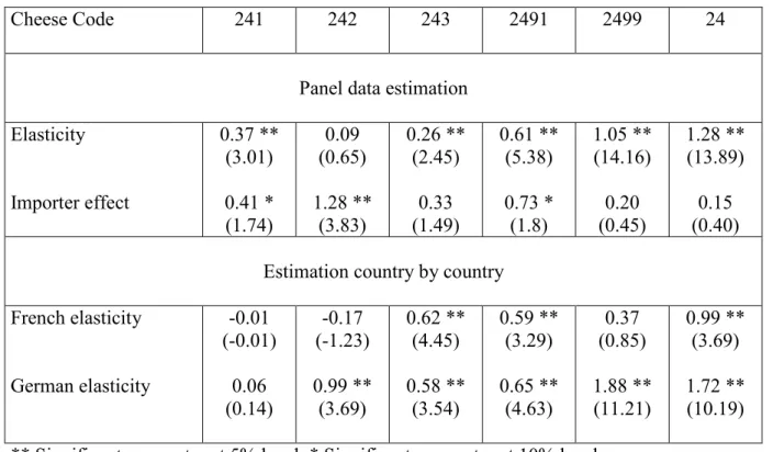
The estimation results of the CES demands (equation 3) are reported in table 1. We first simultaneously estimate French and German imports from other EU countries and test for the presence of an importer (fixed/random) specific effect.7 The results are mixed: for 3 types of cheese, the importer specific effect is not significant, while for the 3 others, it is significant. The estimated elasticities of substitution have all the expected positive sign and five of them are statistically significant. Surprisingly, the highest elasticity of substitution is obtained with the most aggregated product (whole cheese). The elasticity values are quite low but comparable to Surry, Herrard and Le Roux (2002). In order to appreciate the impact on these elasticity estimates of imposing identical CES forms, we also provide in table 1 the results of CES estimation by country. In the case of Germany, all estimated substitution elasticities have the expected positive sign and are significant while two French substitution elasticities are negative but however not statistically significant. It appears that imposing the same substitution elasticity among these two importers does not systematically lead to an average of country elasticities. For instance, on grated cheese (241), the estimation country by country leads to non significant substitution elasticities, while the panel data estimation concludes to positive and significant substitution elasticity which is larger than the country ones. The result is quite different for processed cheese (242). The imposed common substitution elasticity is intermediate between the French and German estimates but it lacks statistical significance, while the German estimate is statistically significant. Regarding blue veined cheese (243), the estimation by country reveals positive and significant substitution elasticities. The imposed
7
This panel data estimation has been conducted with both ML and GME, and both procedures provide the same results.
common substitution elasticity is still positive and statistically significant but the estimated value is much lower than the country ones. Accordingly, we are not able on this dataset to reveal a clear pattern of bias resulting from the imposition of symmetric CES functional forms for preferences.
To sum up these first results, once the assumption of CES preferences is adopted, the additional assumption of symmetric preferences made in gravity models is partly supported. In case of contradiction, the direction of bias on elasticity estimates is unclear.
3.2.2. Estimation of the AI demand systems without zeros
Let’s now consider the analysis of other assumptions (homothetic, monotone and CES preferences). In order to lighten the analysis, we will present the estimation results for two cheese products only: the aggregate cheese product where the monotony issue is absent and one disaggregated product where some trade flows are null. Let’s start with the estimation of the AI demand system for the whole cheese. Results of these estimation are reported in table 2 for France and table 3 for Germany. Rather than providing the whole parameter estimates, we provide substitution and expenditure elasticities for the year 1996 and for the three main exporters in each case. The standard errors have been computed with the delta method.
In these two tables, we report the elasticity estimates and their t-student first without concavity imposed, then with concavity imposed on all points, and finally with concavity imposed on the γij parameters. On the French dataset, it appears that substitution elasticities vary by pairs of countries and some expenditure elasticities are statistically different from one. More precisely, the substitution elasticities between Dutch and Italian cheeses on the one hand, between Dutch and German cheeses on the other hand are positive and statistically different from zero, while the substitution elasticity between Italian and German cheeses is not significant. Accordingly, the assumption of constant elasticity of substitution between pairs of goods is not supported, if the benchmark is the AI demand system. Imports of Italian and Dutch cheeses are clearly non homothetic, with expenditure elasticities of (around) 1.3 and 0.3 respectively, while the student test does not reject the assumption of homotheticity for French imports of German cheese. Thus, both assumptions of homothetic and CES preferences are rejected in the case of French cheese.
Regarding the effects of imposing concavity, our tests lead us to adopt a rank one for the T~t
matrix and thus the resulting AI demand system is slightly (rather than semi) flexible. Despite this huge restriction (only 9 free substitution parameters in our 10 good setting), it is remarkable to note that this does not significantly alter the elasticity estimates. Finally, the imposition of concavity on all data points or on the γij parameters leads to qualitatively identical results.
With the German dataset, results are of a different nature. In particular, with or without concavity imposed, all expenditure elasticities are not statistically different from one. We are thus not able to reject homothetic demand system. In addition, the way we impose the concavity conditions does matter. On the other hand, we still observe different substitution elasticities between pairs of countries. Dutch and Denmark cheeses appear to be close net substitutes for German importers, while Italian and Dutch ones are complements.
Finally, it is interesting to compare these AI estimation results with the CES ones. In table 1, it appears that substitution elasticities by German importers are roughly twice those of French importers. In tables 2 and 3, it again appears that substitution elasticities by German importers are in absolute values larger than the French ones. But the similarity between the two estimations stops when we observe that Italian and Dutch cheeses are complements in the German preference structure, while they are substitute in the French preference structure. To sum up this second group of results, using the AI demand system as the true benchmark, the assumption of constant elasticities of substitution is not supported by both datasets, while the assumption of homothetic preferences is partially supported.
3.2.3. Estimation of the AI demand systems with zeros
We finally take as one example the French imports of processed cheese (242) in order to consider the monotony issue. Over the 1988-2004 period, there are no imports of Denmark processed cheese in the years 1999, 2000 and 2002. When we previously estimated the CES demand system, we ignored these years. If we want to take them into account, we must fix a price and we need to assume that the French import price of Danish processed cheese is given by the maximum over all EU importers of this particular cheese. Table 4 reports the results of two estimations of this AI demand system. In the first case, the zero trade flows are incorporated in the estimation as any other trade flows. In the second case, the zero trade
flows are treated like in Golan, Perloff and Shen (2001). In both cases, concavity is imposed on the γij parameters.
It appears that the specification of zero trade flows as in Golan, Perloff and Shen (2001) does not significantly alter the estimations compared to the results without monotony imposed. This result is not particularly surprising because there are quite few zero trade values and above all, Arndt, Liu and Preckel (1999) already showed that simple OLS estimates may be as good as Heckman estimates which neglect the existence and role of virtual prices.
4. Concluding comments
The primary purpose of this article is the econometric estimation of price elasticity of food trade functions. We investigate the relevance of the gravity approach, nowadays extensively used, in order to simultaneously measure these elasticities as well as the trade costs. The approach is based on the assumptions of symmetric, monotone, homothetic, CES preferences. We test all these assumptions using European intra-trade so as to disregard the problem of trade costs identification. We focus on cheese as an a priori differentiated food product. The estimation of demand systems is performed using Generalized Maximum Entropy estimators which easily allow us to impose both concavity and monotony conditions. In a general way, all assumptions made on preferences by the gravity approach are not supported by our data set. The bias induced on the estimated price elasticities is not univocal.
These econometric results lead us to put some warnings on the use of the price elasticities derived from current gravity equations. The joint assumptions of symmetric, monotone, homothetic CES preferences are certainly highly convenient in order to simultaneously estimate trade costs and preferences of consumers on foreign products. But they are likely to bias both estimations (AvW, 2004). In order to overcome this issue, we suggest that more general gravity equations should be devised. The specification of quasi homothetic demand systems (with the Linear Expenditure System) is a first good step to consider.
References
Alston, J., C. Carter, R. Green, and D. Pick. (1990). Whither Armington Trade Model ? American Journal of Agricultural Economics, 72:455-467.
Anderson, J.E. (1979). A Theoretical Foundation for the Gravity Equation. The American Economic Review, 69:106-116.
Anderson, J.E., and E. van Wincoop (2003). Gravity With Gravitas: A Solution to the Border Puzzle The American Economic Review, 93:170-192.
Anderson, J.E., and E. van Wincoop. (2004). Trade Costs. Journal of Economic Literature, 42:691-751.
Arndt, C., S. Liu, and P. V. Preckel. (1999). On Dual Approaches to Demand Systems Estimation in the Presence of Binding Quantity Constraints. Applied Economics, 31:999-1008.
Barnett, W. A. (2002). Tastes and Technology: Curvature Is Not Sufficient For Regularity. Journal of Econometrics, 108:199-202.
Barnett, W., and M. Pasupathy. (2003). Regularity of the Generalized Quadratic Production Model: A Counterexample. Econometric Reviews, 22:135-154.
Bergstrand, J. H. (1989). The Generalized Gravity Equation, Monopolistic Competition, and the Factor-Proportions Theory in International Trade. The Review of Economics and Statistics, 71(1):143-153.
Blum, B. S., and A. Goldfarb. (2006). Does the Internet Defy the Law of Gravity ? Journal of International Economics, 70(2):384-405.
Bowen, H., Leamer, E. and L. Sveikauskas. (1987). Multicountry, multifactor tests of the factor abundance theory. American Economic Review, 77(5):791-809.
Cooper, R.J., and K.R. McLaren. (1992). An Empirically Oriented Demand System With Improved Regularity Properties. Canadian Journal of Economics, 25:653-668.
Cranfield J., P.V. Preckel, J.S. Eales, and T.W. Hertel. (2002). Estimating consumer demands across the development spectrum: maximum likelihood estimates of an implicit direct additivity model. Journal of Development Economics, 68(2):289-307.
Dalgin, M, V. Trindade, and D. Mitra. (2006). Inequality, Nonhomothetic Preferences, and Trade: a Gravity Approach. National Bureau of Economic Research Working paper 10800.
de Frahan, B.H., and M. Vancauteren. (2006). Harmonisation of Food Regulations and Trade in the Single Market. European Review of Agricultural Economics, 33:337-360.
Deardorff, A. V. (1998). Determinants of Bilateral Trade: Does Gravity Work in a Neoclassical World ? In The Regionalization of the World Economy. J.A. Frankel, ed Chicago: University of Chicago Press, pp. 7-32.
Deaton, A. S., and J. Muellbauer. (1980). An Almost Ideal Demand System. American Economic Review, 70:312-326.
Diewert, W.E., and T.J. Wales. (1988). A Normalized Quadratic Semiflexible Functionnal Form. Journal of Econometrics, 37:327-342.
−−− (1987). Flexible Functional Forms and Global Curvature Conditions. Econometrica 54:43-68.
Dong D., B.W. Gould, and H.M. Kaiser. (2004). Food Demand in Mexico: An Application of the Amemiya-Tobin Approach to the Estimation of a Censored Food System. American Journal of Agricultural Economics, 86(4):1094-1107.
Engel C. (2002). Comment on Anderson and Van Wincoop; in Brookings Trade Forum 2001. Susan Collins and Dani Rodrik, eds. Washington: Brookings Institute.
Evenett, S. J., and W. Keller. (2002). On Theories Explaining the Success of the Gravity Equation. Journal of Political Economy, 110:281-316.
Feenstra, R. C., J.R. James, and A. K. Rose. (2001). Using the Gravity Equation to Differentiate Among Alternative Theories of Trade. Canadian Journal of Economics, 34:430-437.
Gallant, A.R., and E.H. Golub. (1984). Imposing Curvature Restrictions on Flexible Functional Forms. Journal of Econometrics,. 26:295-321.
Golan, A., G. G. Judge, and D. Miller. (1996). Maximum Entropy Econometrics: Robust Estimation With Limited Data. England: John Wiley & Sons Ltd.
Golan, A., G. G. Judge, and J. Perloff. (1997). Estimation and Inference With Censored and Ordered Multinomial Response Data. Journal of Econometrics, 79:23-51.
Golan, A., J. Perloff, and E. Shen. (2001). Estimating a Demand System with Nonnegativity Constraints: Mexican Meat Demand. The Review of Economics and Statistics, 83(3):541-550.
Greene R. (2003). Econometric Analysis. New York : Macmillan Press.
Hassan, M., R.C. Mittelhammer, and T. I. Wahl. (2001). Simulated Maximum Likelihood Estimation of A Consumer Demand System Under Binding Non-Negativity Constraints: An Application To Chinese Household Food Expenditure Data. Working paper, School of Economics Sciences in cooperation with the International Marketing Program for Agricultural Commodities and Trade (IMPACT), Washington State University.
Haveman, J., and D. Hummels. (2004). Alternative Hypotheses and the Volume of Trade: the Gravity Equation and the Extent of Specialization. Canadian Journal of Economics, 37:199-218.
Heien, D., and C. Wessels. (1990). Demand systems estimation with microdata: a censored regression approach. Journal of Business and Economic Statistics, 8:365-371.
Helpman, E., and P.R. Krugman. (1985). Market Structure and Foreign Trade. Cambridge, MA: The MIT Press.
Helpman, E. (1999). The Structure of Foreign Trade. The Journal of Economic Perspectives, 13:121-144.
Hillberry, E.J., and R.H. Balistreri. (2006). Trade Frictions and Welfare in the Gravity Model: How much of the iceberg melts ? Canadian Journal of Economics, 39:247-265.
Hunter, L. (1991). The Contribution of Nonhomothetic Preferences to Trade. Journal of International Economics, 30:345-358.
Ito, S., D.T. Chen, and W. Peterson. (1990). Modeling International Trade Flows and Market Shares for Agricultural Commodities: A Modified Armington Procedure For Rice. Agricultural Economics, 4:315-333.
Karp, L. S., and J. Perloff. (2001) A Synthesis of Agricultural Trade Economics. In Handbook of Agricultural Economics, vol. 2B, Agricultural and Food Policy. The Netherlands : Elsevier Science, Chapter 37, pp. 1945-1998.
Lee, L.F., and M.M. Pitt. (1986). Microeconometric Demand Systems With Binding Nonnegativity Constraints: the Dual Approach. Econometrica, 54:1237-1242.
Markusen, J. R. (1986). Explaining the Volume of Trade: An Eclectic Approach. The American Economic Review, 76:1002-1011.
Miller, D. J., and P. L. Paarlberg. (2001). An Alternative Approach to Determining the Elasticity of Excess Demand Facing the United States. Paper presented at the 2001 Annual Meeting of the American Agricultural Economics Association.
Moschini, G. (1999). Imposing Local Curvature Conditions in Flexible Demand Systems. Journal of Business & Economic Statistics, 4:487-490.
−−− (1998). The Semiflexible Almost Ideal Demand System. European Economic Review, 42:349-364.
Movshuk, O. (2005). International Differences in Consumer Preferences and Trade: Evidence from Multicountry, Multiproduct Data. Working paper, Department of Economics, Toyama University, Japan.
Neary, J. P., and K. W. S. Roberts. (1980). The Theory of Household Behaviour Under Rationing. European Economic Review, 13:25-42.
Ryan, D. L., and T. J. Wales. (1999). Flexible and Semiflexible Consumer Demands With Quadratic Engel Curves. The Review of Economics and Statistics, 81(2):277-287.
Sarker, R., and Y. Surry. (2006). Product Differentiation and Trade in Agri-Food Products: Taking Stock and Looking Forward. Journal of International Agriculture Trade and Development, 2(1):39-78.
Seale, J., A. Regmi, and J. Bernstein. (2003). International Evidence on Food Consumption Patterns. USDA Technical Bulletin, 1904.
Segerson, K. and T. D. Mount. (1985). A Non-Homothetic Two-Stage Decision Model Using AIDS. The Review of Economics and Statistics, 67(4):630-639.
Sheldon, I. (2005). Monopolistic Competition and Trade: Does the Theory Carry Any Empirical ‘Weight’? Paper presented at the 2005 Winter Meeting of the International Agricultural Trade Research Consortium, San Diego, California.
Surry, Y., N. Herrard, and Y. Le Roux. (2002). Modelling Trade in Processed Food Products: an Econometric Investigation for France. Review of Agricultural Economics, 29(1):1-27. Tchamourliyski, Y. (2002). Distance and Bilateral Trade: The Role of Non-Homothetic
Van Akkerren, M., G. Judge, and R. Mittelhammer. (2002). Generalized Moment Based Estimation and Inference. Journal of Econometrics, 107:127-148.
Wolff H., Heckelei T., R. Mittelhammer. (2004). Imposing curvature and monotony on flexible functional forms: an efficient regional approach. Working paper presented at the Econometric Society North American Summer Meetings.
Winters, L. A. (1984). Separability and the Specifications of Foreign Trade Functions. Journal of International Economics, 17:239-263.
Table 1. Econometric Estimation Of Substitution Elasticity With CES Demands On Different Kinds of Cheese
Cheese Code 241 242 243 2491 2499 24
Panel data estimation Elasticity Importer effect 0.37 ** (3.01) 0.41 * (1.74) 0.09 (0.65) 1.28 ** (3.83) 0.26 ** (2.45) 0.33 (1.49) 0.61 ** (5.38) 0.73 * (1.8) 1.05 ** (14.16) 0.20 (0.45) 1.28 ** (13.89) 0.15 (0.40) Estimation country by country
French elasticity German elasticity -0.01 (-0.01) 0.06 (0.14) -0.17 (-1.23) 0.99 ** (3.69) 0.62 ** (4.45) 0.58 ** (3.54) 0.59 ** (3.29) 0.65 ** (4.63) 0.37 (0.85) 1.88 ** (11.21) 0.99 ** (3.69) 1.72 ** (10.19) ** Significant parameter at 5% level, * Significant parameter at 10% level
Student test in parentheses. The importer specific effect pertains to Germany. Cheese codes are explained in footnote 6.
Table 2. Substitution And Expenditure Elasticities Of French Imports Of Total Cheese From Its Main Exporters Estimated With The AI Demand System With/Without Concavity Imposed
Substitution elasticities Exporters
(share)
Italy Netherlands Germany
Expenditure elasticities Belgium (5.7%) -1.06 (-0.65) -1.05 (-0.77) 0.66 (0.43) 1.42 (1.22) 1.41 (1.42) 1.61 (1.19) -1.43 (0.79) -1.47 (-0.97) -0.43 (-0.23) 1.64 (2.43) ** 1.63 (2.85) ** 1.30 (1.02) Italy (19.6%) 1.56 (1.51) 1.58 (1.81) * 2.11 (2.12) ** -1.03 (-0.68) -1.08 (-0.84) -1.27 (-0.83) 1.33 (2.13) ** 1.32 (2.48) ** 1.37 (2.36) ** Netherlands (36.0%) 3.65 (2.68) ** 3.66 (3.22) ** 4.81 (3.27) ** 0.25 (-5.21) ** 0.25 (-6.33) ** 0.43 (-4.23) ** Germany (23.2%) 1.08 (0.34) 1.07 (0.36) 1.03 (0.11) ** Significant parameter at 5% level, * Significant parameter at 10% level
In each cell, the first line gives the estimate without concavity imposed. The second line gives the estimate with concavity imposed on all points. The third line gives the estimates with concavity imposed on the γij parameters.
Student test in parentheses. For the expenditure elasticities, we report the t-student associated to the hypothesis of unitary income elasticities.
Table 3. Substitution And Expenditure Elasticities Of German Imports Of Total Cheese From Its Main Exporters Estimated With The AI Demand System With/Without Concavity Imposed
Substitution elasticities Exporters
(share)
Italy Netherlands France
Expenditure elasticities Denmark (13.3%) 3.27 (0.43) 5.82 (1.00) 8.49 (1.06) 8.12 (2.75) ** 7.98 (3.18) ** 8.85 (3.51) * 5.57 (2.20) ** 4.56 (2.19) ** 1.01 (0.45) 0.90 (-0.19) 0.94 (-0.15) 0.97 (-0.11) Italy (7.5%) -7.09 (-2.00) ** -5.06 (-1.77) * -2.46 (-0.75) 2.15 (0.52) 4.12 (1.38) 0.81 (0.23) 0.85 (-0.21) 1.14 (0.25) 1.49 (0.94) Netherlands (41.9%) 0.15 (0.11) -0.15 (-0.14) 0.99 (1.08) 1.19 (0.61) 1.14 (0.55) 1.02 (0.13) France (31.1%) 0.75 (-1.10) 0.76 (-1.31) 0.98 (-0.15) ** Significant parameter at 5% level, * Significant parameter at 10% level
In each cell, the first line gives the estimate without concavity imposed. The second line gives the estimate with concavity imposed on all points. The third line gives the estimates with concavity imposed on the γij parameters.
Student test in parentheses. For the expenditure elasticities, we report the t-student associated to the hypothesis of unitary income elasticities.
Table 4. Substitution And Expenditure Elasticities Of French Imports Of Processed Cheese From Its Main Exporters Estimated With The Concave AI Demand System With/Without Monotony
Substitution elasticities Exporters
(share)
Denmark United Kingdom Germany
Expenditure elasticities Belgium (8.0%) 129.24 (3.05) ** 98.94 (3.11) ** 8.72 (2.39) ** 8.59 (2.17) ** 1.20 (0.68) 1.23 (0.65) 0.47 (-0.94) 0.36 (-1.04) Denmark (0.1%) -28.88 (-1.75) * -20.89 (-1.86) * -8.48 (-1.35) -5.64 (-1.32) -1.62 (-1.59) -0.97 (-1.66) United Kingdom (15.8%) 0.71 (0.77) 0.74 (0.80) 1.03 (0.17) 1.05 (0.27) Germany (68.5%) 1.09 (1.15) 1.09 (1.22) ** Significant parameter at 5% level, * Significant parameter at 10% level
In each cell, the first line gives the estimate without monotony imposed. The second line gives the estimate with monotony imposed as explained by Golan, Perloff and Shen (2001). In the two cases, concavity is imposed on the γij parameters.
Student test in parentheses. For the expenditure elasticities, we report the t-student associated to the hypothesis of unitary income elasticities.
Working Papers INRA – Unité ESR Rennes
WP02-01 Tariff protection elimination and Common Agricultural Policy reform: Implications of changes in methods of import demand modelling. Alexandre GOHIN, Hervé GUYOMARD, Chantal LE MOUËL (March 2002)
WP02-02 Reducing farm credit rationing: An assessment of the relative effectiveness of two government intervention schemes. Laure LATRUFFE, Rob FRASER (April 2002)
WP02-03 Farm credit rationing and government intervention in Poland. Laure LATRUFFE, Rob FRASER (May 2002)
WP02-04 The New Banana Import Regime in the European Union: A Quantitative Assessment. Hervé GUYOMARD, Chantal LE MOUËL (July 2002)
WP02-05 Determinants of technical efficiency of crop and livestock farms in Poland. Laure LATRUFFE, Kelvin BALCOMBE, Sophia DAVIDOVA, Katarzyna ZAWALINSKA (August 2002)
WP02-06 Technical and scale efficiency of crop and livestock farms in Poland: Does specialisation matter? Laure LATRUFFE, Kelvin BALCOMBE, Sophia DAVIDOVA, and Katarzyna ZAWALINSKA (October 2002)
WP03-01 La mesure du pouvoir de vote. Nicolas-Gabriel ANDJIGA, Frédéric CHANTREUIL, Dominique LEPELLEY (January 2003)
WP03-02 Les exploitations agricoles polonaises à la veille de l’élargissement : structure économique et financière. Laure LATRUFFE (March 2003)
WP03-03 The Specification of Price and Income Elasticities in Computable General Equilibrium Models: An Application of Latent Separability. Alexandre GOHIN (April 2003)