HAL Id: cea-01171610
https://hal-cea.archives-ouvertes.fr/cea-01171610v2
Preprint submitted on 21 Aug 2015
HAL is a multi-disciplinary open access archive for the deposit and dissemination of sci-entific research documents, whether they are pub-lished or not. The documents may come from teaching and research institutions in France or abroad, or from public or private research centers.
L’archive ouverte pluridisciplinaire HAL, est destinée au dépôt et à la diffusion de documents scientifiques de niveau recherche, publiés ou non, émanant des établissements d’enseignement et de recherche français ou étrangers, des laboratoires publics ou privés.
NUCLEAR SPIN NOISE IN NMR REVISITED
Guillaume Ferrand, Gaspard Huber, Michel Luong, Hervé Desvaux
To cite this version:
Guillaume Ferrand, Gaspard Huber, Michel Luong, Hervé Desvaux. NUCLEAR SPIN NOISE IN NMR REVISITED. 2015. �cea-01171610v2�
1
N
UCLEAR SPIN NOISE IN
NMR
REVISITED
Guillaume Ferrand,1 Gaspard Huber,2 Michel Luong,1 Hervé Desvaux2,a)
1. Laboratoire d'ingénierie des systèmes accélérateurs et des hyperfréquences, SACM, CEA, Université Paris-Saclay, CEA/Saclay, F-91191 Gif-sur-Yvette, France.
2. Laboratoire Structure et Dynamique par Résonance Magnétique, NIMBE, CEA, CNRS, Université Paris-Saclay, CEA/Saclay, F-91191 Gif-sur-Yvette, France.
a) herve.desvaux@cea.fr
Abstract
The theoretical shapes of nuclear spin-noise spectra in NMR are derived by considering a receiver circuit with finite preamplifier input impedance and a transmission line between the preamplifier and the probe. Using this model, it becomes possible to reproduce all observed experimental features: variation of the NMR resonance linewidth as a function of the transmission line phase, nuclear spin-noise signals appearing as a ``bump’’ or as a ``dip’’ superimposed on the average electronic noise level even for a spin system and probe at the same temperature, pure in-phase Lorentzian spin-noise signals exhibiting non-vanishing frequency shifts. Extensive comparisons to experimental measurements validate the model predictions, and define the conditions for obtaining pure in-phase Lorentzian-shape nuclear spin noise with a vanishing frequency shift, in other words, the conditions for simultaneously obtaining the Spin-Noise and Frequency-Shift Tuning Optima.
I. Introduction
Nuclear spin noise in NMR was initially predicted by Bloch in 1946 [1] and first detected at the end of the eighties by Sleator et al. using a SQUID for sensitive detection of the nuclear quadrupolar resonance of 35Cl at 4.2K [2, 3]. Later, McCoy and Ernst [4], and Leroy and Guéron [5], independently
reported the observation of nuclear spin noise of protonated solvents using room temperature liquid-state NMR spectrometers. They took benefit of the narrow resonance lines of liquid-state NMR transitions and the strong coupling between large nuclear magnetization and the detection coil. There are two origins of nuclear spin noise in NMR. The first corresponds to the quantum fluctuation of the transverse magnetization and the second to the incoherent radiofrequency (RF) excitations of the longitudinal magnetization inducing in turn the appearance of transverse magnetization [3]. The RF excitations are produced by the Nyquist noise of the electronic detection circuit. Since the electronic circuit is resonant at the Larmor frequency, tiny magnetization fluctuations can be amplified when the nuclear magnetization is significantly coupled to the detection circuit. Consequently, the phenomenon of nuclear spin noise in NMR is strongly correlated to radiation damping [6, 7, 8], that is, the RF magnetic feedback field created by the current in the detection coil
2
induced by the precessing transverse magnetization. This feedback field is expected to be in quadrature to the precessing magnetization for a perfectly tuned electronic circuit [9], inducing only broadening of the observed NMR signals for small flip-angle excitation pulses. Electronic mistuning lifts the perfect quadrature between the feedback field and the transverse magnetization whose NMR signatures are the previously mentioned signal broadening and a frequency shift of the observed NMR resonance frequency (frequency pushing) [10, 11].
After these early observations, nuclear spin noise has not attracted large attention from the NMR community, except for particular detection schemes dedicated to the monitoring of restricted numbers of spins [12, 13, 14]. Indeed, for usual NMR experiments with 1016 - 1020 spins, the
coherent detection after RF excitation is several orders of magnitude more sensitive than noise detection scheme. Recently, the situation has changed [8, 15]. Detection or influence of nuclear spin noise were at the heart of studies of the initiation of spontaneous multiple maser emissions of hyperpolarized 129Xe [16, 17, 18], for the observation of other maser emissions [19, 20] or for the
capability of continuous monitoring of hyperpolarized species without destroying the transient magnetization through RF excitations [21, 22]. Also, the appearance of cold-probes with very large quality factors 𝑄 has facilitated the detection of nuclear spin noise. It has, for instance, allowed the direct acquisition of images without RF excitations [23] or the detection of thermally polarized 13C
nuclear spin noise [24]; even 2D-NMR spectra based on spin-noise detection scheme have been reported [25]. Nevertheless, with consequences on a much broader audience these fundamental studies are mainly put forward problems of tuning of the electronic circuit [26]. Essentially when the electronic circuit is tuned at the Larmor frequency and matched at 50 Ω with respect to the emission circuit, a condition known as Conventional Tuning Optimum, CTO [27], the shapes of the nuclear spin-noise signals usually appear as distorted Lorentzian, contrary to the theoretical predictions [4, 10], revealing a mistuning according to the reception circuit. Conversely, when the electronic circuit was tuned for observing pure in-phase Lorentzian shapes for the nuclear spin-noise signals, an increase of the detected signals in conventional pulsed experiments was obtained with potentially an increase of signal-to-noise ratios [26]. This tuning condition was named Spin-Noise Tuning Optimum, SNTO [27]. More recently some of us have shown that even in conditions where spin-noise signals of pure in-phase Lorentzian shapes are observed, non-vanishing frequency pushing effects can be detected [28]. The tuning conditions, for which this frequency shift vanishes, have been named Frequency Shift Tuning Optimum. It was also demonstrated [28] that these experimental observations of the difference between FSTO and SNTO were not compatible with the theoretical predictions of references [4, 10].
The present article is devoted to solving this contradiction. We consider the complete detection circuit with a finite input impedance of the preamplifier and the effect of the transmission line length
3
between the probe and the preamplifier as in Ref. [29]. We, in particular, take into account the noise produced by the preamplifier impedance which is fed back to the coil through the transmission line. The combination of the two last terms plays a key role for explaining the experimental observation. After Section II, dedicated to Materials and Methods, in Section III, theoretical models are described, providing evidence of the importance of both electronic elements. After a short description of the classical theory (Section III.A), in Section III.B it is predicted that, depending on the transmission line and preamplifier impedance, the radiation damping contribution can strongly vary altering the nuclear spin resonance line-width and potentially inducing, for a perfectly tuned system (SNTO condition), the appearance of a ''bump'' rather than the usual ''dip'' for the nuclear spin-noise signal superimposed on the average electronic noise level for a thermally equilibrated spin system and a classical probe. In addition in Section III.C the RF excitations affecting the nuclear susceptibility induced by Nyquist noise due to the preamplifier impedance are considered: a model allowing the numerical calculation of the nuclear spin-noise spectra is developed. Conversely to the model of Section III.B, using this model FSTO and SNTO conditions are not always simultaneously fulfilled. Finally, in Section III.D a mathematical framework is introduced which allows us to formally obtain the general shape of the nuclear spin-noise resonance. In this framework, it becomes possible to demonstrate that FSTO and SNTO conditions can differ, such an effect results from magnetization excitations induced by noise fluctuations within the preamplifier impedance combined with dephasing effects due to the transmission line. Section IV is devoted to the careful validation of the model: nuclear spin-noise spectra have been simulated using the measured electronic components and directly confronted to experimental measurements. In Section V, several aspects of the derivation are discussed; in particular an equation which can be used for determining physically relevant parameters is introduced. Finally, conclusions are drawn in Section VI.
II. Materials and methods
NMR experiments have been performed on a Bruker Avance DRX500 spectrometer equipped with a 5-mm inverse broadband probe-head with z-gradient, operating at 500 MHz for proton. In order to freely modify the preamplifier-probehead coupling, a phase shifter (ARRA inc., model 2448A), previously calibrated by connection to a vector network analyzer, was introduced between the preamplifier and the cable to the probe. The phase shift reference 𝜙0 has been arbitrarily chosen.
The total phase from the probe to the preamplifier 𝜙 was defined by 𝜙 = 𝜙0+ 𝜓, where 𝜓 was the
variable phase difference introduced by the phase shifter, which conveniently simulates a transmission line of variable length.
4
For the quantitative validation between the numerical simulations and experiments, spectra were acquired at 293 K on a solution composed of 90% acetone and 10% deuterated chloroform for magnetic field lock purposes. First using a network analyzer directly connected to the probe, the capacitors 𝐶𝑡 and 𝐶𝑚 were set to ensure a probe circuit resonance frequency equal to the Larmor
frequency and a perfect matching to 50 Ω. If the tuning and matching capacitors 𝐶𝑡 and 𝐶𝑚 were
adjusted with the Bruker’s wobulation routine, the values would have depended on the phase shift, preventing detailed comparisons between experiments and numerical simulations. This new procedure corresponds to the Probe Impedance Matching Optimum (PIMO) [30], the capacitances were kept constant and only the phase shift 𝜓 between the preamplifier and the probe was changed by adjusting the phase shifter from 0 to 191.9°, by increments of 10.1°. Due to the impedance of the TR-switch, the obtained capacitor values did not correspond to the CTO condition as determined using the Bruker’s wobulation routine. For each of the 20 𝜓 values, a spin-noise spectrum and a classical spectrum acquired thanks to a small-excitation pulse were acquired, and the measurements were compared to the values derived from numerical simulations performed with SciLab. All parameters used in these simulations were the experimental ones: the different unknowns (inductance, resistance of coil, 𝐶𝑡, 𝐶𝑚, input impedance of the preamplifier) have, in particular, been
determined from external measurements performed with the network analyzer.
Spin-noise spectra were composed of 12 FIDs of 512k points, each acquired in 52.4 s. The latter were post-processed using SciLab with the sliding windows protocol for ensuring a final real resolution of about 0.7 Hz with a zero-fill factor of 2 and the optimal signal-to-noise ratio in the given amount of time [8, 21]. To avoid artifacts due to non-perfect SNTO conditions (leading to a mixture of absorptive and dispersive Lorentzian in spin-noise line-shapes), the resonance frequency for extracting frequency shifts and the line-widths of 12𝐶𝐻
3𝐶𝐶𝐶𝐻3 signal were determined from the
5
III. Spin-Noise Theory
A. Classical theory of nuclear spin-noise line-shape
Figure 1: Schematic of the detection circuit with the different noise sources 𝑈𝑒, 𝑈𝑐 and 𝑈𝑠, for the preamplifier, coil and spin
sources, respectively. The resistance 𝑅𝑐 and the inductance 𝐿 of the coil are affected by the presence of the nuclear
susceptibility, represented by 𝑅𝑠 and 𝐿𝑠. The reference planes labeled with circled numbers allow the definition of the
intermediate impedances and transmission matrices. 𝑍𝑖𝑖 and 𝑍𝑖𝑖 denote the impedances seen at plane 𝑖 from the
preamplifier (left side) and from probe (right side), respectively.
Classically [9], the detection circuit is modeled by a coil (𝐿, 𝑅𝑐) with a capacitor chip 𝐶𝑡 in parallel and
the voltage is measured at the position of plane 3 of Figure 1. This measurement condition implicitly assumes a very high preamplifier input impedance, 𝑍𝑒, directly connected at position of plane 3 in
parallel to the capacitor chip 𝐶𝑡, i.e. without matching capacitor 𝐶𝑚 and transmission line. Following
Mc Coy and Ernst [4], as a result of the spin resonance, the inductance of the coil becomes:
𝐿 → 𝐿 + 𝐿𝑠−𝑗𝑅𝜔 = 𝐿𝑠 (1 + 𝜂𝜂). (3.1)
The parameter 𝜂 corresponds to the filling factor, and 𝜂 = 𝜂′− 𝑗𝜂′′ is the nuclear susceptibility:
�𝜂′ = 𝜇0
2 𝛾 ℳ𝑧 𝑑(𝛿𝜔), 𝜂′′ = 𝜇2 𝛾 ℳ0 𝑧 𝑎(𝛿𝜔).
(3.2)
In equation (3.2), 𝜇0 is the magnetic permeability of free space, ℳ𝑧, the longitudinal nuclear
magnetization which can be enhanced relative to thermal equilibrium magnetization ℳ0 by
hyperpolarization techniques [21, 22] or saturated by RF irradiation [4], 𝛾 the magnetogyric ratio and 𝑎(𝛿𝜔) and 𝑑(𝛿𝜔) the absorptive and dispersive resonance line shapes, respectively:
⎩ ⎨ ⎧𝑎(𝛿𝜔) = 𝜆2 𝜆22 + (𝜔 − 𝜔 0)2, 𝑑(𝛿𝜔) = 𝜔 − 𝜔0 𝜆22 + (𝜔 − 𝜔0)2, (3.3)
with 𝜆2 the transverse self-relaxation rate and 𝜔0 the nuclear spin Larmor resonance frequency.
Then, introducing the quality factor 𝑄 = 𝐿𝜔0/𝑅𝑐, the radiation damping rate 𝜆𝑟 for a given
6 𝜆𝑟 =𝜇2 𝛾 𝜂 𝑄 ℳ0 𝑧 = 𝜂𝑄𝜂 ′′ 𝑎(𝛿𝜔) = 𝜂𝑄𝜂′ 𝑑(𝛿𝜔). (3.4) The radiation damping rate at thermal equilibrium λr0 is defined by equation (3.4) with ℳz= ℳ0.
Due to the presence of the nuclear magnetization, the resistance and inductance of the coil have been replaced in Figure 1 by an equivalent spin-noise resistance and inductance 𝑅𝑐𝑠𝑠 = 𝑅𝑐
(1 +
𝜆𝑟𝑎
(
𝛿𝜔))
and 𝐿𝑐𝑠𝑠 = 𝐿 + 𝑅𝑐𝜆𝑟𝑑(
𝛿𝜔)
/𝜔, respectively. Associated to these resistances, the noisevoltage is defined by 𝑈𝑠𝑠 = 𝑈𝑅+ 𝑈𝑠, where 𝑈𝑠 and 𝑈𝑅 are the noise voltages generated by the spins
and the resistance of the coil, respectively. We denote
𝑊
𝑖 and𝑊
𝑠 their associated spectraldensities: � 𝑊𝑖= 2 𝜋 𝑘𝑏𝑇𝑝𝑅𝑐, 𝑊𝑠=𝜋 𝑘2 𝑏𝑇𝑝𝑅𝑐𝜆𝑟0𝑎(𝛿𝜔). (3.5)
where 𝑇𝑝 is the probe and sample temperature, 𝑘𝑏, the Boltzmann constant, and where we have
used the remark that the spin term is temperature independent since it only depends on the number density of spins [4].
The voltage measurement is performed at the tuning capacitor chip terminals. In these conditions, according to Figure 1, the total spectral density is:
𝑊𝑡 =𝜔2 𝐶1 𝑡2 𝑅𝑐2⋅ 2 𝜋 𝑘𝑏𝑇𝑝 𝑅𝑐 + 2𝜋 𝑘𝑏𝑇𝑝 𝑅𝑐𝜆0𝑟 𝑎(𝛿𝜔) [1 + 𝜆𝑟𝑎(𝛿𝜔)]2+ � 1𝑅𝑐(𝐿𝜔 − (𝐶𝑡𝜔)−1) + 𝜆𝑟𝑑(𝛿𝜔)� 2 (3.6)
Equation (3.6) simplifies when the Larmor resonance frequency, 𝜔0, matches the electronic circuit
resonance frequency, i.e. 𝜔0�𝐿𝐶𝑡 = 1:
𝑊𝑡 =𝜋 ⋅2 𝜔2𝑘 𝐶𝐵𝑇𝑝
𝑡2 𝑅𝑐⋅ �1 −
𝜆𝑟 2 + 2𝜆𝑟𝜆2 − 𝜆𝑟0𝜆2
(𝜔 − 𝜔0)2 + (𝜆𝑟 + 𝜆2)2�.
(3.7) This corresponds to the equation derived by McCoy and Ernst [4] which has also been extended to the case of cold probes [27] or of hyperpolarized species [21].
B. Nuclear spin-noise line shape with a noiseless preamplifier
We consider now a more realistic detection scheme where the input impedance of the preamplifier, 𝑍𝑒, is not infinite [31] (cf. Figure 1). This has two consequences:
• A transmission line between the preamplifier and the probe is added whose length (or the associated phase 𝜙) provides an additional degree of freedom but which may also modify the response of the circuit if the input impedances of the probe and preamplifier are not matched to the transmission line impedance 𝑍0(cf. Figure 1).
7
• The resistance impedance of the preamplifier ℜ(𝑍𝑒) [32] induces a new Nyquist noise
source. This source can excite the nuclear magnetization through the induced current fluctuations due to the preamplifier resistance but in a non-straightforward way since there is no special relation between the impedance of the preamplifier and that of the probe. Assuming, in the present subsection, that the noise temperature of the preamplifier 𝑇𝑒 is close to
zero, the latter contribution to spin noise becomes negligible.
In Figure 1, 𝑍3𝑅
= 1/(𝐺 + 𝑗𝑗)
was defined as the impedance seen by the coil at plane 3.Substituting 𝑋 = 𝐺2 + (𝐶
𝑡𝜔 + 𝑗)2, the spectral density is:
𝑊𝑡 =𝜋 ⋅2 𝑘𝑅𝐵 𝑇𝑝 𝑐 𝑋 ⋅ 1 + 𝜆𝑟0 𝑎(𝛿𝜔) �1 + 𝐺𝑅 𝑐 𝑋 + 𝜆𝑟𝑎(𝛿𝜔)� 2 + �𝐿𝜔𝑅 𝑐 − 𝐶 𝑡𝜔 + 𝑗 𝑋𝑅𝑐 + 𝜆𝑟𝑑(𝛿𝜔)� 2. (3.8)
If 𝑍6𝑖, the impedance seen by the voltage source 𝑈𝑠𝑠 at reference plan 6, is real, then the source is in
resonance with the circuit and the NMR frequency shift vanishes. This corresponds to FSTO condition:
𝐿𝜔 =𝐶𝑡𝜔 + 𝑗𝑋 . (3.9)
In fact, the solution of equation (3.9) depends on the impedance of the preamplifier 𝑍𝑒 and of the
phase of the transmission line 𝜙. In other words, FSTO depends on the transmission line length. Defining an apparent radiation damping rate 𝜆𝑟′:
𝜆𝑟′ = 𝜆𝑟
1 + 𝐺𝑅
𝑐𝑋
. (3.10)
the expression of the spectral density becomes: 𝑊𝑡 =𝜋 ⋅2 𝑘𝐵 𝑇𝑝 𝑅𝑐 𝑋 �1 + 𝐺𝑅 𝑐𝑋� 2⋅ �1 − 𝜆𝑟 ′ 2 + 2𝜆 𝑟 ′𝜆 2 − 𝜆𝑟0𝜆2 (𝜔 − 𝜔0)2 + (𝜆2 + 𝜆𝑟′)2�. (3.11)
In the specific case where 𝐺 = 𝑗 = 0, i.e. the preamplifier has an infinite impedance such as an open-circuit, then 𝑋 and 𝜆𝑟′ are equal to 𝐶𝑡2𝜔2 and 𝜆𝑟 respectively, and Equation (3.11) reduces to
Equation (3.7).
Finally, the measurement is performed through the voltage, 𝑈𝑧, at the extremities of the preamplifier
input impedance. The measured spectral density can be computed from the voltage spectral density 𝑊𝑡 through the transmission line of impedance 𝑍0 and phase 𝜙 [33, 34]:
𝑊𝑧 = 𝑊𝑡 �cos 𝜙 + 𝑗 cos 𝜙𝑍 1 3𝑖𝐶𝑚𝜔 − 𝑗 𝑍0sin 𝜙 𝑍3𝑖 � 2 . (3.12)
According to equation 3.12, 𝑊𝑧 and 𝑊𝑡 exhibit same resonance line shapes since �cos 𝜙 +
𝑗 cos 𝜙𝑍 1
3𝑅𝐶𝑚𝜔− 𝑗
𝑍0sin 𝜙
𝑍3𝑅 �
2
8
varies slowly compared to 𝑊𝑡 around the Larmor frequency 𝜔0. Furthermore, according to equations
(3.11), in the FSTO condition, under the assumption of vanishing noise temperature of the preamplifier, the shape of 𝑊𝑡, i.e. the spin-noise shape of 𝑊𝑧, is an in-phase Lorentzian and
corresponds to the SNTO condition. Since FSTO and SNTO conditions always match, this model is too simplified for explaining the observed discrepancies reported in Ref. [28].
C. Model with preamplifier noise
To take into account the effects of RF excitations induced by the finite impedance of the preamplifier on the nuclear spins and their consequences on spin-noise spectra (𝑇𝑒 ≠ 0), we shall, in this section
use a transmission matrix, also known as ABCD matrix, approach. The whole system is described by a single matrix 𝑇𝑠𝑠= 𝑇
1𝑇2𝑇3𝑇4𝑠𝑠𝑇5𝑠𝑠 of dimension 2×2. The transmission matrices 𝑇𝑖 are given in
microwave engineering textbooks [34]:
⎩ ⎪ ⎨ ⎪ ⎧ 𝑇 1= � cos 𝜙 𝑗𝑍0sin 𝜙 𝑗 sin 𝜙 𝑍0 cos 𝜙 � , 𝑇 2 = �1 1 𝑗𝐶𝑚𝜔 0 1 � , 𝑇3= � 1𝑗𝐶𝑡𝜔 1� , 𝑇0 4𝑠𝑠= �1 𝑗𝐿𝑐 𝑠𝑠𝜔 0 1 � , 𝑇5𝑠𝑠= �1 𝑅𝑐 𝑠𝑠 0 1 � . (3.13)
The measured voltage 𝑈𝑧 across the preamplifier impedance 𝑍𝑒 is given by:
�𝑈𝑖𝑧 𝑧� = �𝑇 11𝑠𝑠 𝑇12𝑠𝑠 𝑇21𝑠𝑠 𝑇22𝑠𝑠� �𝑈 𝑠𝑠 𝑖𝑠𝑠�, (3.14) where 𝑇𝑖𝑖𝑠𝑠 are elements of matrix 𝑇𝑠𝑠. Introducing 𝑍
𝑒 that relates 𝑈𝑧 and 𝑖𝑧, one obtains [35]:
𝑊𝑧 = �𝑍 𝑍𝑒 𝑒𝑇22𝑠𝑠+ 𝑇12𝑠𝑠�
2
𝑊𝑠𝑠,
(3.15) with 𝑊𝑠𝑠= 𝑊𝑖+ 𝑊𝑠. In the FSTO condition, the result is given by equation (3.12).
Noise contribution from a preamplifier is classically modeled with real part of its input impedance combined to an equivalent temperature 𝑇𝑒 [34]; therefore, the preamplifier noise spectral density is:
𝑊𝑝𝑝 =2𝜋 𝑘𝑇𝑒ℜ(𝑍𝑒). (3.16)
The impedance seen by the preamplifier, 𝑍1𝑖, is given by 𝑍1𝑖 = 𝑇12𝑠𝑠/𝑇22𝑠𝑠, and the contribution of the
preamplifier to the spin-noise spectrum 𝑊𝑝 by:
𝑊𝑝 = � 𝑇12 𝑠𝑠 𝑍𝑒𝑇22𝑠𝑠+ 𝑇12𝑠𝑠� 2 ⋅2𝜋 𝑘𝑇𝑒ℜ(𝑍𝑒). (3.17) Comparison of Eqs. (3.15) and (3.17) indicates a different dependence on the nuclear susceptibility of these two noise contributions since 𝑇12𝑠𝑠 depends on 𝐿𝑠𝑠𝑐 and 𝑅𝑐𝑠𝑠. In addition to the probe, spins and
preamplifier noise contributions to the measured spectra, there is an extra component which is constant over the frequency range and does not interact either with the probe or the spins: the
9
constant noise of the preamplifier and the noise coming from other external sources between the preamplifier and the analog-to-digital converter (ADC), hereafter denoted 𝑊𝑒𝑒𝑡. It introduces an
offset in the spectra and cannot be neglected if comparisons to experimental spectra are carried out. Hence, the simulated spin-noise power spectrum should be written:
𝑊𝑡𝑡𝑡=2𝑘𝑇𝜋𝑝|𝑇12 𝑠𝑠|2
(𝑅𝑐+ 𝑅𝑠𝑠) + 𝑇𝑇𝑒𝑝ℜ(𝑍𝑒)|𝑇22 𝑠𝑠|2
|𝑍1𝑖𝑇22𝑠𝑠+ 𝑇12𝑠𝑠|2⋅ |𝑇22 𝑠𝑠|2 + 𝑊 𝑒𝑒𝑡.
(3.18)
D. Pseudo-Lorentzian shape of the spin-noise spectrum
For extracting NMR relevant parameters without having access to all electronic parameters (the usual situation in particular with cold probes) we show here that the general shape of nuclear spin noise is a generalized Lorentzian function (called Lorentzian function) [35]. The pseudo-Lorentzian function, Λ[𝑝, 𝑞](𝑥) with 𝑝 and 𝑞 complex-valued parameters, is defined by:
Λ[𝑝, 𝑞](𝑥) = 1 +1 + 𝑗𝑞𝑥𝑝 (3.19)
This function has several properties [35] but an important one for the present purpose, is the capability to rewrite any pseudo-Lorentzian function with a real-value parameter |𝑞|2/ℜ(𝑞) and a
shift (−ℑ(𝑞)/|𝑞|2) according to the 𝑥 parameter:
For 𝑞 ≠ 0, Λ[𝑝, 𝑞](𝑥) = 1 +ℜ(𝑞)1 𝑝𝑞⋆
1 + 𝑗 |𝑞|ℜ(𝑞) �𝑥 −2 ℑ(𝑞)|𝑞|2�.
(3.20)
The total impedance of the coil with the nuclear spin contributions can therefore be split into two contributions: the coil inductance 𝑗𝐿𝜔 and the residual impedance of the coil, 𝑍𝑟𝑠, defined by:
𝑍𝑟𝑠 = 𝑅𝑐+ 𝑗𝐿𝜔𝜂(𝜂′− 𝑗𝜂′′). (3.21)
Using the definition of the pseudo-Lorentzian function (3.19), 𝑍𝑟𝑠 can be written as:
𝑍𝑟𝑠 = 𝑅𝑐⋅ Λ �𝜆𝜆𝑟 2, − 𝜔0 𝜆2� � 𝜔 − 𝜔0 𝜔0 �. (3.22) We consider the transmission matrix 𝑇𝑖 with 𝑇𝑖 = 𝑇
1𝑇2𝑇3𝑇𝑖, where 𝑇𝑖 is the transmission matrix of
the coil inductance 𝐿. The impedance 𝑍1𝑖 seen by the preamplifier is:
𝑍1𝑖 =𝑍𝑟𝑠𝑇11 𝑖 + 𝑇
12𝑖
𝑍𝑟𝑠𝑇21𝑖 + 𝑇22𝑖.
(3.23) After little algebra with transmission matrices and using several properties of the pseudo-Lorentzian function one can show that the impedance 𝑍1𝑖 is a pseudo-Lorentzian function whatever the values
of 𝑇𝑖. The Johnson-Nyquist noise, 𝑊
10 𝑊𝑧 =2𝜋 𝑘𝑏𝑇𝑝ℜ(𝑍1𝑖) |𝑍𝑒|
2
|𝑍1𝑖+ 𝑍𝑒|2,
(3.24) Introducing the preamplifier noise source, 𝑊𝑝, and the external noise source, 𝑊𝑒𝑒𝑡, as in equation
(3.18), provides an equation for the measured spin noise: 𝑊𝑡𝑡𝑡=2𝜋 𝑘𝐵⋅ �𝑇𝑒ℜ(𝑍𝑒)|𝑍1𝑖| 2 |𝑍1𝑖+ 𝑍𝑒|2 + 𝑇pℜ(𝑍1𝑖)|𝑍𝑒|2 |𝑍1𝑖+ 𝑍𝑒|2 � + 𝑊 𝑒𝑒𝑡. (3.25)
Using the properties of the real part, Equation (3.25) can be written as: 𝑊𝑡𝑡𝑡=𝜋 𝑘2 𝐵⋅ 𝑇𝑒⋅ ℜ ⎝ ⎛ 𝑍𝑒𝑍1𝑖 𝑍𝑒 + 𝑍1𝑖⋅ � 𝑇𝑝 𝑇𝑒 ⋅ 𝑍𝑒 + 𝑍1𝑖 𝑍𝑒 + 𝑍1𝑖 � ⋆ ⎠ ⎞ + 𝑊𝑒𝑒𝑡. (3.26)
Since it can be shown that the term 𝑍𝑒𝑍1𝐿
𝑍𝑒+𝑍1𝐿 is a pseudo-Lorentzian function, we shall denote its
associated 𝑞 parameter as 𝑞0. Using properties of the pseudo-Lorentzian function, 𝑊𝑡𝑡𝑡 can be
written as [35]:
𝑊𝑡𝑡𝑡=2𝜋 𝑘𝐵⋅ 𝑇𝑒 ⋅ ℜ �𝑍𝑓⋅ Λ�𝑝𝑓, 𝑞0�� + 𝑊𝑒𝑒𝑡, (3.27)
where 𝑍𝑓 and 𝑝𝑓 are constant parameters that depend on 𝑍1𝑖, 𝑍𝑒 and the noise temperatures of the
probe 𝑇𝑝 and the preamplifier 𝑇𝑒. This demonstrates that the nuclear spin-noise spectrum is the real
part of a pseudo-Lorentzian function. Accordingly, there exist solutions for which this function reduces to the pure in-phase Lorentzian, which corresponds to the SNTO condition.
As a consequence, in the SNTO condition, the observed resonance frequency can be different from the Larmor frequency (this corresponds to the case where ℑ(𝑞0) ≠ 0). The frequency offset, given by
Equation (3.20), is ℑ(𝑞0)
|𝑞0|2𝜔0, and is exactly equal to the frequency shift given by Guéron’s model [10].
Hence, the frequency shift of the chemical spectra corresponds exactly to the frequency offset seen on the spin-noise spectra. This result can be extended to the case of any noise-source temperatures. Optimal tuning condition corresponds to the simultaneous achievement of SNTO and FSTO. Mathematically, this is equivalent to:
𝐹𝐹𝑇𝐶 = 𝐹𝑆𝑇𝐶 ⟺ �ℑ�𝑍ℑ(𝑞0) = 0,
𝑓𝑝𝑓� = 0.
(3.28) Equation (3.28) describes the entire set of solutions of the SNTO problem, the general analysis of which is difficult. However, a sufficient (but not necessary) condition is given by:
�ℑ(𝑇ℑ(𝑍𝑖) = 0,
𝑒) = 0. ⇒ 𝐹𝑆𝑇𝐶 = 𝐹𝐹𝑇𝐶.
(3.29) In other words, if the impedance of the preamplifier and the four coefficients of the transmission matrix 𝑇𝑖 are real, then the SNTO condition is satisfied and the resonance frequency of the peak
11
IV. Features of the nuclear spin-noise spectra
A. Dip or bump in spin-noise spectra at thermal equilibrium
Assuming a negligible noise contribution of the preamplifier to the spin dynamics (𝑇𝑒 = 0), equation
(3.11) reveals several features of spin-noise line-shapes as a function of preamplifier impedances and transmission lengths in the SNTO condition. Firstly, the line width (𝜆2 + 𝜆′𝑟) is affected by the
impedance 𝑍3𝑖 at the FSTO condition (equation (3.9)). Consequently it varies with the impedance of
the preamplifier 𝑍𝑒, and 𝜙. Secondly, the intensity of the spin-noise signal also depends on this
impedance and can, at particular angles 𝜙, give different results from the model of McCoy and Ernst [4]. Indeed, the impedance 𝑍3𝑖 can be small for particular phases of the transmission line since the
measured impedances of the preamplifier are of the order of tens of Ω. If 𝐺 is large, i.e. 𝜆𝑟′ ≪ 𝜆𝑟, the
circuit is designed in such a way that radiation damping is strongly reduced. The situation can even be such that 𝜆𝑟′ 2 + 2𝜆𝑟′𝜆2− 𝜆0𝑟𝜆2 becomes negative (for very large 𝐺, this corresponds to 𝜆0𝑟 > 𝜆𝑟′).
Then instead of observing a decrease of noise at the Larmor frequency for a perfectly tuned probe (SNTO) at thermal equilibrium as predicted by the classical theory (equation (3.7)), an increase of noise, that is a bump and not the usual dip, is theoretically predicted and experimentally observed [29]. Conversely, if the impedance 𝑍3𝑖 is large, 𝜆𝑟 ≃ 𝜆𝑟′, the behavior becomes very similar to the
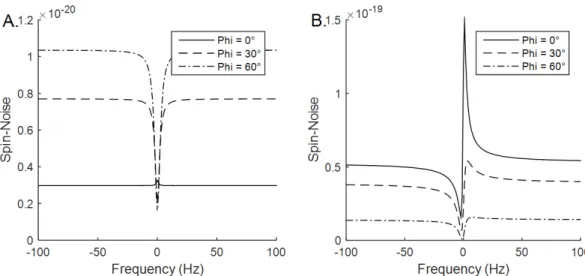
predictions of McCoy and Ernst [4] or Guéron [10]. The transition from low impedance to high impedance can be easily obtained with a phase shift of 90°. Figure 2A illustrates this transition from a dip to a bump for three values of the transmission line phase 𝜙.
Figure 2: Numerical simulation of spin-noise spectra for different 𝜙 parameters, under FSTO condition. On panel A, the noise temperature of the preamplifier is set to 0 K (no preamplifier noise) and Equation (3.12) was used. On panel B, the noise temperature of the preamplifier is set to 150 K and Equation (3.20) with a vanishing external noise (𝑊𝑒𝑒𝑡= 0). The
12
Figure 2A shows the nuclear spin-noise spectra using the no-noise preamplifier model described in equation (3.12) and assuming FSTO conditions. Perfect absorptive Lorentzian shapes are obtained with an average out-of-resonance noise level, linewidth and Larmor frequency noise level which depend on the transmission line. In particular, for 𝜙 = 0°, a bump is predicted instead of the usual dip, in agreement with a previous report [29].
To explore a more realistic case, for which the effect of preamplifier noise was also considered, the calculation was carried out in the framework of the transmission matrices (Section III.C). We assumed 𝑊𝑒𝑒𝑡= 0 and 𝑇
𝑒 = 150 𝐾, typical of low-noise preamplifiers. The result, given by equation
(3.18), is shown in Figure 2B. The introduction of a noise source from the preamplifier induced different nuclear spin-noise shapes (not always pure in-phase Lorentzian) even if FSTO condition (Equation (3.9)) was assumed. Also, the average noise level was amplified by about one order of magnitude. The preamplifier contribution, even for low temperature noise, appears much higher than the probe contribution. Highly asymmetrical line shapes (for instance, for 𝜙 = 30°) were observed. Moreover, the small bump seen on Figure 2A for 𝜙 = 0° was strongly enhanced with the appearance of a non-symmetrical high bump. The present simulations in FSTO conditions and taking into account the preamplifier noise which excites nuclear magnetization, lead to nuclear spin noise not always corresponding to SNTO conditions. This is the first numerical illustration that FSTO and SNTO conditions cannot be matched simultaneously. The comparison between the used assumptions for obtaining these two simulations (Figures 2A and 2B) indicates that different FSTO and SNTO conditions can be obtained only if noise produced by the preamplifier impedance can be fed back to the coil through the transmission line inducing excitations of the nuclear spins.
B. Experimental validation of the theoretical model
In Figure 3, are reported 20 spin-noise spectra acquired for a series of 𝜓 values and a probe tuned and matched at 50 Ω using a vector network analyzer (PIMO conditions [30]). For 𝜓 = 10.1° and 𝜓 = 101°, the nuclear spin-noise spectra appeared as almost perfect in-phase Lorentzian shapes, for the first one as a bump and the second one as a dip. On these two spectra the best least-squares fit to Equation (3.18) gave 𝜆2= 21.7 𝐻𝐻, 𝜆𝑟 = 148.2 𝐻𝐻, 𝑇𝑒 = 175 𝐾 and 𝑊𝑒𝑒𝑡 which represented
about 13% of the noise produced by the probe far from the NMR spin resonance. Finally, the value of 𝜙0 was optimized, (𝜙0 = −8.0°), revealing that the second spectrum of Figure 3 corresponds to
𝜙 = 2.1°.
In a next step, using the best fit parameters and the given 𝜙 values, for all panels the simulated curves obtained using Equation (3.18) were recomputed and superimposed (green lines) on the experimental measurements (red lines) (Figure 3). Good agreement is observed, which proves that
13
spin-noise spectra are well described by Equation (3.18) and validates the theoretical model of Section III.C. This set of experiments shows that starting from the PIMO tuning condition it was possible to reach the SNTO condition by modifying the cable length between the preamplifier and the probe.
14
Figure 3: Experimental nuclear spin-noise spectra of acetone acquired on a classical probe tuned at PIMO in red lines. The only differences between these 20 spectra were the variable transmission line phases 𝜓 which were incremented by step of 10.1°. SNTO conditions were found for 𝜓 = 10.1° with a bump signal and 𝜓 = 101° for which a dip was observed. Using the electronic component parameters, the four values 𝝀𝒓, 𝝀𝟐, 𝑇𝑝, 𝑊𝐴𝐴𝐶 were optimized on these two spectra. The best-fit curves
computed using Equation (3.18) were superimposed. Then for all the others experimental spectra, the simulated spectra were recomputed by only changing the phase values 𝜓 and keeping all the other parameters constant. The simulated curves are also superimposed in green lines. A good agreement can be observed.
15
C. Obtaining the same FSTO and SNTO conditions
The last issue to address is how to practically ensure simultaneous FSTO and SNTO conditions. Solving equation (3.28) was impossible in the general case, we have therefore chosen to address the sufficient condition (3.29). We verified experimentally that the PIMO condition almost satisfied equation (3.29) for two different phases 𝜙. As a result, the conditions PIMO and FSTO entailed the condition SNTO.
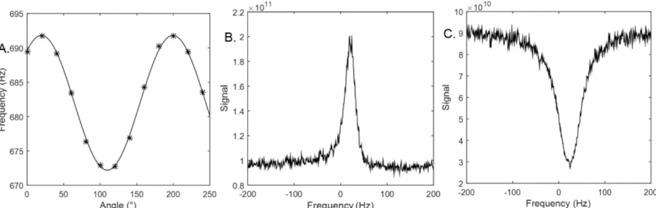
Starting from the PIMO condition, we explored the variation of peak resonance frequencies on spectra acquired after small-excitation pulses for 𝜓 ranging from 0 to 190° in 10° steps. It can be shown that this variation is described by a sinusoid [35]. The mean shift corresponded to the Larmor frequency and allowed the determination of phases 𝜓 for which the FSTO condition was fulfilled. An illustration of this dependence is reported in Fig. 4A. The best-fit to a sinusoid of the experimental measurements allowed the determination of the FSTO conditions which were fulfilled for 𝜓 = 64.5° and 154.5°.
Figure 4: Panel A: Variation, as a function of the transmission line phase 𝜓, of the nuclear resonance frequency of acetone measured on spectra acquired after small excitation pulses, for a probe tuned according to the PIMO condition. Asterisks show the experimental measurements and the solid line represents the best-fit sinusoid curve. From this analysis the FSTO conditions could be determined, they corresponded to 𝜓 = 64.5° and 𝜓 = 154.5°. The two nuclear spin-noise spectra acquired with these phases are shown in panels B and C, respectively. Their shapes were almost perfect in-phase Lorentzian with a bump and a dip, respectively and a linewidth also affected by the transmission line phase.
Finally, for these two phases, spin-noise spectra were acquired and the results are reported in Figure 4B and C. They corresponded to almost perfect in-phase Lorentzian shapes with a dip for 𝜓 = 154.5° and a bump for 𝜓 = 64.5°. As a consequence they correspond to the SNTO condition and proved that starting from PIMO condition and by monitoring the frequency shift variation as a function of the angle 𝜙 it was possible to simultaneously ensure FSTO and SNTO.
Careful shape analysis nevertheless reveals that the SNTO condition was not perfectly achieved for 𝜓 = 64.5°. The peak is slightly asymmetric. We have therefore analyzed the reliability of the FSTO=SNTO condition and its stability, using the numerical simulation approach based on
16
transmission matrices (Section III.C). Starting from PIMO condition and changing the tuning or the matching capacitance by 0.5% induced the disappearance of the capability of obtaining same FSTO and SNTO conditions. In the case of probe and sample cooled down at 𝑇𝑝= −60°C, a difference
between FSTO and SNTO has been experimentally shown [28]. We assumed that the only effect of this cooling was the reduction of the resistance 𝑅𝑐 by a factor 2. The threshold on the tuning
capacitance for obtaining same PIMO, FSTO, and SNTO conditions was then reduced from 0.5% to 0.1%. Finally, the threshold for cold probe with a 𝑄 factor of 8000 and thus a resistance of 𝑅𝑐= 0.01 Ω, was found to be 0.02%, a value typically below of what could be achieved based on
mechanical and electronic precisions. This result illustrates that even if in theory it should be possible to match different tuning conditions (PIMO, FSTO, SNTO) even on a cold probe, it can be expected to be difficult to achieve on an experimental point of view.
For the two optimal configurations for which FSTO and SNTO are simultaneously fulfilled, either a bump or a dip with an in-phase Lorentzian line shape and no frequency shift are observed. For these spectra, the signal-to-noise ratio can be defined as:
𝐹𝑆𝑅 = |𝐹0− 𝐹𝜎 <>|
𝑆0
(4.1) Where 𝐹<> is the average noise level out-of-resonance and 𝐹0 and 𝜎𝑆0 are the noise level at nuclear
resonance and its associated standard deviation which scales as the square-root of the number 𝑠 of scans: 𝜎𝑆0∝ 𝐹0√𝑠 . Denoting 𝑘 = 𝐹0/𝐹<>, the signal-to-noise ratio scales as |1 − 1/𝑘|√𝑠 [8, 21].
For a bump, this SNR is limited to √𝑠, while for a dip it can reach larger value if 𝑘 < 0.5. Such a condition can experimentally be obtained by reducing the noise contribution of the preamplifier and increasing the radiation damping rate. These last two conditions are fulfilled for the dip configuration. As a whole, the dip configuration appears, in general, as the best one for observing nuclear spin noise.
V. Discussion
A. Comparison with the McCoy and Ernst theory
In Section III.D, we have shown that in a restricted range of frequency around the Larmor frequency, the spin-noise spectrum can be represented by 𝑎 ℜ �Λ[𝑝, 𝑞] �𝜔−𝜔0
𝜔0 �� where 𝑎 is a real coefficient
and 𝑝 and 𝑞 are complex values. This result proves that in general the shape of the spin-noise spectrum can be represented as a mixture of absorptive and dispersive Lorentzian functions.
17
This is also the case of the classical equation (3.7) derived by McCoy and Ernst [4] and Guéron [10], this explains why it was generally impossible by a simple fitting procedure to evidence the weaknesses of this usual model. Indeed, except for the particular cases where bumps at thermal equilibrium and using classical probe are observed [29], experimental spin-noise spectra can always be described by Equation (3.7) through adjusting 𝜆𝑟, 𝜆2, 𝜔0 and constant noise levels for the coil and
the preamplifier (𝑊𝑐). The alternative way to reveal the weakness of this theory was by showing that
for SNTO condition the frequency shift can experimentally be different from zero [28]. In our model, the observation of a ``bump’’ and non-vanishing frequency shift for SNTO are now explained, since a Lorentzian function with a complex-valued parameter 𝑞 can be transformed into a pseudo-Lorentzian function with real-valued parameter 𝑞 through a translation in the frequency domain (equation (3.20)), that is with a frequency shift contribution. We consequently have a mathematical definition of the SNTO condition which is not dependent on matching the resonance frequency of the electronic circuit and the Larmor frequency, the latter corresponds to the physical definition of FSTO condition. In that sense, the contradiction between experiments and theoretical derivations put forward in reference [28] is definitively solved.
B. A phenomenological equation
For practical applications of NMR spectroscopy, in particular using a cold probe, it is desirable to have a simplified model reproducing the essential characteristics described by the general one presented here. The usual inability to mathematically distinguish the general model from the McCoy and Ernst’s model provides clues for obtaining a phenomenological equation which could be used to fit the experimental measurements and to obtain relevant parameters (transverse relaxation and radiation damping rates, Larmor resonance frequencies, offset in tuning). If one considers a spectrum acquired at SNTO, the FSTO condition is not automatically fulfilled. According to Equation (3.20), the term 𝛿𝜔 = 𝜔 − 𝜔0 in Equation (3.8) has to be replaced by 𝛿𝜔′= 𝛿𝜔 − 𝜁, where 𝜁 is the frequency shift
dependent on the difference between the Larmor frequency and the frequency corresponding to the FSTO condition, 𝜔FSTO. The second correction consists in noting that the SNTO condition does not
require a constant noise level out-of-resonance. Since the frequency ranges of NMR spectra are much narrower than the bandwidths of detection circuit, a linear dependence seems sufficient to represent this variation of the average noise level. This finally leads to the following phenomenological equation:
𝑊𝑡 = 𝐴 ⋅ 1 + 𝜆𝑟
0 𝑎(𝛿𝜔′)
[1 + 𝜆𝑟′ 𝑎(𝛿𝜔′)]2+ [Δ + 𝜆𝑟′ 𝑑(𝛿𝜔′)]2+ 𝑗𝛿𝜔 + 𝐶.
18
The parameter Δ represents the tuning-dependent frequency offset between the actual resonance frequency for spin-noise and the perfect SNTO condition leading to a phase-mixed Lorentzian resonance shape [28].
C. Equivalent electronic circuit
The theoretical derivation also physically and mathematically defines what is meant by the FSTO condition. It corresponds to an equivalent impedance, 𝑍6𝑖, at the reference plan #6, which is purely
real. In terms of radiation damping physics this is equivalent to a current in phase with the source voltage produced by the precessing magnetization [9], inducing a feedback field in quadrature to the precessing magnetization. Mathematically the FSTO condition corresponds to Equation (3.9) which appears to be dependent on the tuning capacitance but also on all the other components of the electronic reception circuit. It is particularly dependent on the length of the transmission line through the phase 𝜙. This is in agreement with previous experimental observations which have shown the existence of a large number of tuning and matching conditions for obtaining SNTO and have revealed the dependence on the transmission line of the SNTO conditions [28, 29].
Finally, the general demonstration and calculation carried out here, prove that the spin-dynamics interaction between the magnetization and the electronic circuit can be modeled by a simple equivalent RLC circuit [9]. Obviously, the effective quality factor is not given by the quality factor of the coil 𝑄 = 𝐿𝜔/𝑅𝑐 but depends on all electronic components of the reception circuit, explaining the
appearance of the modified radiation damping rate 𝜆𝑟′ in Equations (3.10) and (5.1) and the
introduction of an apparent quality factor 𝑄′ = 𝑄 / �1 + 𝐺
𝑖𝑐𝑋�, also introduced experimentally for
explaining the difference between the extracted 𝑄 parameters and the ones claimed by the probe manufacturers [8, 28, 29, 36].
VI. Conclusion
Nuclear spin noise in NMR has been observed for the first time more than 25 years ago and described by McCoy and Ernst’s equation [4] which was derived assuming that all properties of the electronic circuit leading to radiation damping can be reproduced by an equivalent RLC circuit. Recently, it was experimentally shown that the predictions of this model are incorrect since pure in-phase spin-noise spectra can be obtained with a non-vanishing frequency shift, i.e. a radiation damping field not in quadrature to the magnetization [28]. The model developed in the present article solves this difficulty by introducing a careful description of the detection circuit. The discrepancy appears to result from magnetization excitations due to the fluctuating current within
19
the finite impedance of the preamplifier coupled to the coil through a transmission line which has the incorrect length. The quality of this model was assessed by extensive comparisons between simulated and experimental spectra performed for a large series of transmission line phases 𝜙. We also theoretically predict experimental spin-noise spectra with pure in-phase Lorentzian shape and a bump rather than the usual dip in the average noise level. The latter solution appears as the best one in terms of signal-to-noise ratio per time unit for spin-noise detection. We also show the influence of the preamplifier impedance and transmission line phase on the observed resonance linewidth. Finally, the model reveals that experimental conditions exist for which the FSTO and SNTO conditions match but are almost unattainable with a cold probe due to uncertainties in the determination of the tuning and matching capacitor values.
Calculation of spin-noise spectra with the present model requires the knowledge of all electronic components of the detection circuit, a feature which is feasible on a room temperature probe but which is usually beyond what an NMR spectroscopist can do on a commercial cold probe. As a consequence, we have introduced a phenomenological equation valid for one spin-species which allows one to best-fit experimental measurements in order to have access to NMR parameters (effective radiation damping rate, relaxation rate, and resonance frequency).
Acknowledgments
This research was supported the Agence Nationale de Recherche (project IMAGINE, ANR project 12-IS04-0006).
References
[1] F. Bloch, Phys. Rev. 70, 460-474 (1946).
[2] T. Sleator, E. L. Hahn, C. Hilbert and J. Clarke, Phys. Rev. Lett. 55, 1742-1745 (1985). [3] T. Sleator, E. L. Hahn, C. Hilbert and J. Clarke, Phys. Rev. B 36, 1969-1980 (1987). [4] M. A. McCoy and R. R. Ernst, Chem. Phys. Lett. 159, 587-593 (1989).
[5] M. Guéron and J. L. Leroy, J. Magn. Reson. 85, 209-215 (1989). [6] N. Bloembergen and R. V. Pound, Phys. Rev. 95, 8-12 (1954). [7] M. P. Augustine, Prog. NMR Spectrosc. 40, 111-150 (2002). [8] H. Desvaux, Prog. NMR Spectrosc. 70, 50-71 (2013).
20
[9] A. Vlassenbroek, J. Jeener and P. Broekaert, J. Chem. Phys. 103, 5886-5897 (1995). [10] M. Guéron, Magn. Reson. Med. 19, 31-41 (1991).
[11] D. A. Torchia, J Biomol NMR 45, 241-244 (2009).
[12] F. Jelezko, T. Gaebel, I. Popa, M. Domhan, A. Gruber and J. Wrachtrup, Phys. Rev. Lett. 93, 130501 (2004).
[13] T. Staudacher, F. Shi, S. Pezzagna, J. Meijer, J. Du, C. A. Meriles, F. Reinhard and J. Wrachtrup, Science 339, 561-563 (2013).
[14] S. A. Crooker, D. G. Rickel, A. V. Balatsky and D. L. Smith, Nature 431, 49-52 (2004). [15] N. Müller, A. Jerschow and J. Schlagnitweit, eMagRes 2, 237-243 (2013).
[16] D. J.-Y. Marion, G. Huber, P. Berthault and H. Desvaux, ChemPhysChem 9, 1395-1401 (2008). [17] D. J.-Y. Marion, P. Berthault and H. Desvaux, Eur. Phys. J. D 51, 357-367 (2009).
[18] V. Henner, H. Desvaux, T. Belozerova, D. J. Y. Marion, P. Kharebov and A. Klots, J. Chem. Phys. 139, 144111 (2013).
[19] H.-Y. Chen, Y. Lee, S. Bowen and C. Hilty, J. Magn. Reson. 208, 204-209 (2011). [20] A. Jurkiewicz, Chem. Phys. Lett. 623, 55-59 (2015).
[21] H. Desvaux, D. J. Y. Marion, G. Huber and P. Berthault, Angew. Chem. Int. Ed. 48, 4341-4343 (2009).
[22] P. Giraudeau, N. Müller, A. Jerschow and L. Frydman, Chem. Phys. Lett. 489, 107-112 (2010). [23] N. Müller and A. Jerschow, Proc. Natl. Acad. Sci., USA 103, 6790-6792 (2006).
[24] J. Schlagnitweit and N. Müller, J. Magn. Reson. 224, 78-81 (2012).
[25] K. Chandra, J. Schlagniweit, C. Wohlschlager, A. Jerschow and N. Müller, J. Phys. Chem. Lett. 4, 3853-3856 (2013).
[26] D. J.-Y. Marion and H. Desvaux, J. Magn. Reson. 193, 153-157 (2008).
[27] M. Nausner, J. Schlagnitweit, V. Smrečki, X. Yang, A. Jerschow and N. Müller, J. Magn. Reson. 198, 73-79 (May 2009).
[28] M. Pöschko, J. Schlagnitweit, G. Huber, M. Nausner, M. Horničáková, H. Desvaux and N. Müller, ChemPhysChem 15, 3639-3645 (2014).
[29] E. Bendet-Taicher, N. Müller and A. Jerschow, Conc. Magn. Reson. B 44, 1-11 (2014).
[30] G. Ferrand, M. Luong, G. Huber and H. Desvaux, Conc. Magn. Reson. B in press, DOI: 10.1002/cmr.b.21277 (2015).
21
[32] ℜ and ℑ describe the real part and imaginary part of a complex-valued parameter, respectively. [33] P. Horowitz and W. Hill, The Art of Electronics, (Cambridge University Press, Cambridge, 1989). [34] D. M. Pozar, Microwave Engineering, 4th ed. (Wiley, 2012).
[35] See supplemental material at [URL] for detailed demonstrations and other experimental
illustrations.
[36] J. Schlagnitweit, S. W. Morgan, M. Nausner, N. Müller and H. Desvaux, ChemPhysChem 13, 482-487 (2012).
1
Nuclear spin noise in NMR, revisited
Supplemental material
Guillaume Ferrand,
1Gaspard Huber,
2Michel Luong,
1Hervé Desvaux
2,a)1. Laboratoire d'ingénierie des systèmes accélérateurs et des hyperfréquences, SACM, CEA, Université Paris-Saclay, CEA/Saclay, F-91191 Gif sur Yvette, France.
2. Laboratoire Structure et Dynamique par Résonance Magnétique, NIMBE, CEA, CNRS, Université Paris-Saclay, CEA/Saclay, 91191 Gif sur Yvette, France.
a) herve.desvaux@cea.fr
I.
Supplementary elements for the theoretical developments
A. Demonstration of Equation (3.15)
In the general case, if 𝑇 is a transmission matrix transforming the voltage and intensity 𝑈1+, 𝑖1+ into
𝑈2+, 𝑖2+, i.e. �𝑈2 + 𝑖2+� = �𝑇 11 𝑇12 𝑇21 𝑇22� �𝑈 1+
𝑖1+�, for the inverse transmission matrix, by convention, the signs
of the intensities have to be inverted (𝑖1−= −𝑖1+). Since for here-considered electronic components
the system is symmetrical, the inverse transmission matrix is: �𝑈𝑖1− 1−� = �𝑇 22 𝑇12 𝑇21 𝑇11� �𝑈 2− 𝑖2−�. (𝐴. 1)
Figure S.1 Schematic of a transmission matrix transforming 𝑍1 to 𝑍2.
Considering the scheme of Figure S.1, from the impedance 𝑍1 and the transmission matrix 𝑇 the
impedance 𝑍2 can be computed:
𝑍2 =𝑈𝑖2 2 =
𝑍1𝑇11+ 𝑇12
𝑍1𝑇21+ 𝑇22. (𝐴. 2)
2 𝑍1=𝑍𝑍2𝑇22+ 𝑇12
2𝑇21+ 𝑇11. (𝐴. 3)
According to the sign convention of Figure 1, the ratio 𝑈𝑠𝑠/𝑖𝑠𝑠 is equal to −𝑍6𝐿, which can be
computed thanks to Equation A.3. The result can be applied to Equation 3.14, replacing 𝑖𝑠𝑠 by
𝑈𝑠𝑠/−𝑍6𝐿. Finally, 𝑈𝑧 is obtained:
𝑈𝑧 =𝑍 𝑍𝑒𝑈𝑠𝑠
𝑒𝑇22𝑠𝑠+ 𝑇12𝑠𝑠. (𝐴. 4)
This was used to obtain the spectral density (Equation 3.15).
Preamplifiers are characterized by noise factors 𝐹𝑑𝑑, expressed in dB, which describes the
signal-to-noise ratio degradation between the input and the output. The relation between 𝐹𝑑𝑑 and the
equivalent temperature 𝑇𝑒 used in the article (Equation 3.16 and numerical applications, is:
𝑇𝑒 = 𝑇0�10𝐹𝑑𝑑/10− 1�, (𝐴. 5)
with 𝑇0 a reference temperature equal to 290 K.
B. Demonstration of the pseudo-Lorentzian shape (Equation 3.27)
There are two useful properties of pseudo-Lorentzian functions Λ, defined by Equation 3.19: 1 𝑎 ⋅ Λ[𝑝, 𝑞] + 𝑏 = 1 𝑎 + 𝑏 ⋅ Λ�−𝑝 ⋅ 𝑎 𝑏 + 𝑎(1 + 𝑝) , 𝑞 ⋅ 𝑏 + 𝑎 𝑏 + 𝑎(1 + 𝑝)�, (𝐵. 1) And: 𝑎 ⋅ Λ[𝑝, 𝑞] + 𝑏 = (𝑎 + 𝑏) ⋅ Λ �𝑝 ⋅𝑎 + 𝑏 , 𝑞𝑎 �. (𝐵. 2) Equation 3.23 of the main text can be written as:
𝑍1𝐿 =𝑍𝑟𝑠𝑇11 𝑅 + 𝑇 12𝑅 𝑍𝑟𝑠𝑇21𝑅 + 𝑇22𝑅 = 𝑇11𝑅 𝑇21𝑅 + �𝑇12𝑅 −𝑇22 𝑅𝑇 11𝑅 𝑇21𝑅 � ⋅𝑍 1 𝑟𝑠𝑇21𝑅 + 𝑇22𝑅 (𝐵. 3)
where 𝑍𝑟𝑠 is a pseudo-Lorentzian function as shown in the main text. By using successively the two
relations B.1 and B.2, it becomes clear that 𝑍1𝐿 is a pseudo-Lorentzian function.
Starting from Equation 3.26, and defining 𝑍1𝑓 =𝑍𝑍𝑒𝑒+𝑍𝑍1𝐿1𝐿= 𝑍𝑒 − 𝑍𝑒
2 𝑍𝑒+𝑍1𝐿 and 𝐾2𝑓 = 𝑇0 𝑇𝑒⋅𝑍𝑒+𝑍1𝐿 𝑍𝑒+𝑍1𝐿 = 1 + �𝑇0𝑇𝑒−1�⋅𝑍𝑒
𝑍𝑒+𝑍1𝐿 , we can show using Equations B.1 and B.2 that these two terms, 𝑍1𝑓 and 𝐾2𝑓 are
3
the same 𝑞 parameter which we denote 𝑞0 since they have the same denominator. We define 𝑝𝑓1
and 𝑝𝑓2 as the 𝑝 parameters of 𝑍1𝑓 and 𝐾2𝑓, respectively and 𝑍1∞ and 𝐾2∞, the values of 𝑍1𝑓 and
𝐾2𝑓 for far off-resonance condition (𝜔 → ∞). Then, the product 𝑍1𝑓𝐾2𝑓⋆ can be written as:
𝑍1𝑓𝐾2𝑓⋆ = 𝑍1∞𝐾2∞⋆ �1 +1 + 𝑗𝑞𝑝𝑓1 0𝑥 + 𝑝𝑓2⋆ 1 − 𝑗𝑞0𝑥 + 𝑝𝑓1𝑝𝑓2⋆ 1 + 𝑞02𝑥2�. (𝐵. 4)
First, if 𝑞0 is real-valued, we have:
⎩ ⎪ ⎨ ⎪ ⎧ ℜ �𝑝𝑓2⋆ 𝑍1∞𝐾2∞⋆ 1 − 𝑗𝑞0𝑥 � = ℜ � 𝑝𝑓2𝑍1∞⋆ 𝐾2∞ 1 + 𝑗𝑞0𝑥 � , ℜ �𝑍1∞1 + 𝑞𝐾2∞⋆ 𝑝𝑓1𝑝𝑓2⋆ 02𝑥2 � = ℜ�𝑍1∞𝐾2∞ ⋆ 𝑝 𝑓1𝑝𝑓2⋆ �ℜ �1 + 𝑗𝑞1 0𝑥� . (𝐵. 5)
According to Equations B.4 and B.5:
�if: 𝑍𝑒𝑒= 𝑍1∞𝐾2∞⋆ +
𝑝𝑓1𝑍1∞𝐾2∞⋆ + 𝑝𝑓2𝑍1∞⋆ 𝐾2∞+ ℜ�𝑝𝑓1𝑝𝑓2⋆ 𝑍1∞𝐾2∞⋆ �
1 + 𝑗𝑞0𝑥 ,
then: ℜ�𝑍𝑒𝑒� = ℜ�𝐾1𝑓𝑍2𝑓⋆ �.
(𝐵. 6)
It demonstrates that 𝑊𝑡𝑡𝑡 in Equation 3.26 can be written as the real part of a pseudo-lorentzian
function, 𝑍𝑒𝑒.
Now, if 𝑞0 is not real-valued (ℑ(𝑞0) ≠ 0), by using Equation 3.20 the transformation of 𝑥 into
𝑥′ = 𝑥 −ℑ(𝑒0)
|𝑒0|2 allows the restoration of real 𝑞0
′ = |𝑞
0|2/ℜ(𝑞0) parameter. Noting that ℑ(𝑞0) =
ℑ(−𝑞0⋆), thus Equation B.4 remains valid, after the transformation of 𝑥, 𝑞0, 𝑝𝑓1 and 𝑝𝑓2 into a set
𝑥′, 𝑞
0′, 𝑝𝑓1′ and 𝑝𝑓2′ according to Equation 3.20. Equations B.5 and B.6 must be modified with these
new parameters. Finally, Equation 3.20 can be used in Equation B.6 to transform 𝑞0′𝑥′ into |𝑒0|2
ℜ(𝑒0)�𝑥 −
ℑ(𝑒0)
|𝑒0|2�. This demonstrates the pseudo-lorentzian shape of the spin-noise resonance
whatever the value of the 𝑞0 parameter and whatever the noise temperature of the preamplifier.
C.
McCoy and Ernst’s equation and the pseudo-Lorentzian function
Equation 3.6 introduced by McCoy and Ernst was used for several decades for describing spin-noise spectra.1 This equation can indeed be written as a pseudo-Lorentzian function. In order to prove it,
let 𝑍𝑐 and 𝑍𝑙 be defined as: 𝑍𝑐 = 𝑅𝑐+ 𝑗𝑗𝜔 − 𝑗(𝐶𝑡𝜔)−1 and 𝑍𝑙 = 𝑅𝑐𝜆𝑟�𝑎(𝛿𝜔) + 𝑗𝑗(𝛿𝜔)�. With
4 𝑊𝑡 =2𝜋 ⋅𝜔𝑘𝑑2𝐶𝑇𝑝 𝑡2⋅ ℜ(𝑍𝑐) + 𝜆𝑟 0 𝜆𝑟ℜ(𝑍𝑙) |𝑍𝑐+ 𝑍𝑙|2 . (𝐶. 1)
Similar expression is obtained for Equation 3.8 (model with non-infinite input impedance of the preamplifier). Equation C.1 can be expressed in a similar way as Equation 3.25 and thus the same transformation can be used. Indeed:
𝑊𝑡 =2𝜋 ⋅𝜔𝑘2𝐶𝑑𝑇𝑝 𝑡2𝑅𝑐2⋅ ℜ ⎝ ⎛ 𝑅𝑐2 𝑍𝑐+ 𝑍𝑙⋅ � 𝜆0𝑟 𝜆𝑟𝑍𝑙+ 𝑍𝑐 𝑍𝑐+ 𝑍𝑙 � ⋆ ⎠ ⎞. (𝐶. 2) Equation C.2 can be written as:
𝑊𝑡 =2𝜋 ⋅𝜔𝑘2𝐶𝑑𝑇𝑝 𝑡2𝑅𝑐2⋅ ℜ ⎝ ⎜ ⎛ 𝑅𝑐2 𝑍𝑐+ 𝑍𝑙⋅ ⎝ ⎜ ⎛𝜆0𝑟 𝜆𝑟�1 − �1 − 𝜆𝑟0 𝜆𝑟� 𝑍𝑐 𝑍𝑐+ 𝑍𝑙 � ⎠ ⎟ ⎞ ⋆ ⎠ ⎟ ⎞ . (𝐶. 3)
Since 𝑍𝑙=𝜆2−𝑗(𝜔−𝜔𝑅𝑐𝜆𝑟 0), 𝑍𝑐+ 𝑍𝑙 is a pseudo-Lorentzian function defined by:
𝑍𝑐+ 𝑍𝑙 = (𝑅𝑐+ 𝑗(𝑗𝜔 − (𝐶𝑡𝜔)−1))Λ �𝑅 𝑅𝑐 𝑐+ 𝑗𝑗𝜔 − 𝑗(𝐶𝑡𝜔)−1⋅ 𝜆𝑟 𝜆2, − 𝜔0 𝜆2� � 𝜔 − 𝜔0 𝜔0 � . (𝐶. 4)
According to Equation B.1, with 𝑏 = 0, 𝑍1𝑓 = 𝑅𝑐
2
𝑍𝑐+𝑍𝑙 is a pseudo-Lorentzian function with parameters:
⎩ ⎪ ⎨ ⎪ ⎧ 𝑝1𝑓 = −𝑅𝑐 �𝜆2 𝜆𝑟+ 1� 𝑅𝑐+ 𝜆 2 𝜆𝑟(𝑗𝑗𝜔 − 𝑗(𝐶𝑡𝜔) −1), 𝑞0= − 𝑅𝑐+ 𝑗𝑗𝜔 − 𝑗(𝐶𝑡𝜔) −1 �𝜆2 𝜆𝑟+ 1� 𝑅𝑐+ 𝜆 2 𝜆𝑟(𝑗𝑗𝜔 − 𝑗(𝐶𝑡𝜔) −1)⋅ 𝜔0 𝜆𝑟 . (𝐶. 5)
In the same way, 𝐾2𝑓 =𝜆𝜆0𝑟�1 −
�1−𝜆𝑟0𝜆𝑟�𝑍𝑐
𝑍𝑐+𝑍𝑙 � is a pseudo-Lorentzian function. Especially, if 𝜆𝑟
0 = 𝜆 𝑟,
𝐾2𝑓 = 0, and the nuclear spin-noise shape corresponds to the shape of 𝑍1𝑓 given by Equation C.5.
Otherwise, the development of the Equations is similar to Equation B.6. Whatever the value of 𝜆𝑟0,
the final quality factor is given by 𝑞0 (Equation C.5).
If (𝑗𝜔 − (𝐶𝑡𝜔)−1) = 0, the coefficients 𝑞0, 𝑝1𝑓 and 𝑝2𝑓 are purely real. The quality factor 𝑞0 is given
by: 𝑞0= −𝜆2𝜔+𝜆0𝑟. This corresponds to the quality factor of Equation 3.7. This corresponds to the
5 a frequency shift contribution equal to 𝜁 =ℑ(𝑒0)
|𝑒0| but simultaneously the shape of the spin-noise
resonance is not that of an in-phase Lorentzian function.
D. Demonstration of the sinusoidal shape of Figure 4A
The transmission matrix of a transmission line is given by 𝑇𝐿= �
cos 𝜙 𝑗𝑍0sin 𝜙 𝑗 sin 𝜙
𝑍0 cos 𝜙 �.
In the condition of Equation 3.29 (that is the solution proposed for simultaneous SNTO and FSTO condition), if a phase shift is added to 𝑇𝑅, between the probe and the preamplifier, the total
transmission line is given by the matrix product 𝑇𝐿⋅ 𝑇𝑅. Using Equations B.1 and B.2 for the
transmission matrix product 𝑇𝐿⋅ 𝑇𝑅, where 𝑇𝑅 is real-valued, we observe that the resulting
parameter ℑ(𝑒)|𝑒|2, and thus the frequency shift, is a function of sin 2𝜙. If the impedance of the preamplifier is purely real (as defined in Equation 3.29), then, the final frequency shift ℑ(𝑒0)
|𝑒0|2 also
varies as sin 2𝜙. This demonstrates the sinusoidal shape of the frequency shift, for the specific case of Equation 3.29.
Especially, in the PIMO condition, there is a phase 𝜙0 for which the transmission matrix 𝑇𝑅 verifies
Equation 3.29. In other words, there is a transmission line matrix 𝑇𝐿0 for which ℑ(𝑇𝐿0⋅ 𝑇𝑃) = 0,
where 𝑇𝑃 is the transmission matrix of the probe in PIMO conditions. Consequently, adding a
transmission line 𝑇𝐿 to a probe matched by PIMO is equivalent to adding a transmission line
described by 𝑇𝐿⋅ 𝑇𝐿0−1 to a probe with transmission matrix 𝑇𝑅 that verifies Equation 3.29.
Consequently, ℑ(𝑒0)
|𝑒0|2 varies according to sin(2𝜙 − 2𝜙
0), where 𝜙0 is the phase parameter of 𝑇 𝐿0. This
validates the shape of Figure 4A. For other conditions (especially CTO conditions), we experimentally observed that the shape of ℑ(𝑒0)
|𝑒0|2 is not a sinusoidal function of 𝜙 (see below).
II.
Dependence of the spin-noise spectra on the tuning parameters
As another procedure for exploring the predictions of the theoretical developments, we report here an experimental study for which the probe was not tuned at PIMO but in contrast, the tuning and matching capacitances were adjusted for each phase of the transmission line for ensuring SNTO condition, in a procedure reminiscent to previous studies.2-4
NMR experiments have been performed on a Bruker Avance DRX500 spectrometer equipped with an inverse broad band probehead with z-gradient, operating at 500 MHz for proton. The sample was made of 90% methyl-isopropyl ketone and 10% deuterated benzene for magnetic field lock purpose.
6
Transmission phase were modified by changing the value of the phase shifter angle, placed between the preamplifier and the probe head. This device has been previously calibrated by connection to a transceiver. For each phase shift, the tuning 𝐶𝑡 and matching 𝐶𝑚 capacitors were adjusted in CTO
condition (emission mode). Then keeping the value of 𝐶𝑚 constant, the tuning capacitor 𝐶𝑡 was
adjusted for ensuring SNTO condition (reception mode). For phases between 10 and 35°, it was not possible to adjust 𝐶𝑡, because of a limited accessible range. Also for 𝜓 = 0° the tuning was
achievable with two extreme values of 𝐶𝑡, so the parameter values corresponding to the two
measurements are reported.
After the achievement of this tuning procedure, a classical proton NMR spectrum obtained after a small flip-angle excitation pulse (ca. 7°) and a spin-noise spectrum composed of 8 FIDs, each one containing 512k points acquired in 52.4 s were recorded. From these two spectra, four NMR parameters were extracted: the resonance frequency and thus the frequency shift and the linewidth of 12CH
3CO signal from the classical FID, noise level out-of and at resonance from the noise spectra.
We, indeed, preferred to avoid directly exploiting spin-noise spectra for extracting frequency shifts and linewidths since small offsets relative to perfect SNTO conditions would lead to significant errors in the determination of these two parameters.4 Examples of these spectra acquired after a small
flip-angle excitation pulse and using the nuclear spin-noise scheme are reported in Figure S.2.
Figure S.2. Examples of aliphatic parts of 1H spectra acquired with a small flip-angle excitation pulse (A) on methyl isopropyl ketone (in insert) and with nuclear spin-noise scheme (B). These spectra have been acquired with a phase 𝜓=0° of the phase
shifter. The linewidth and resonance frequency of signal 2 measured on spectrum A were used in the following steps of analysis and the average noise level out-of-resonance (1.90 1011) and at resonance (about 7.7 1010) measured on the
spin-7
noise spectrum (B). A significant frequency shift contribution can easily be detected through the shape of the doublet 3 (see Reference 5).
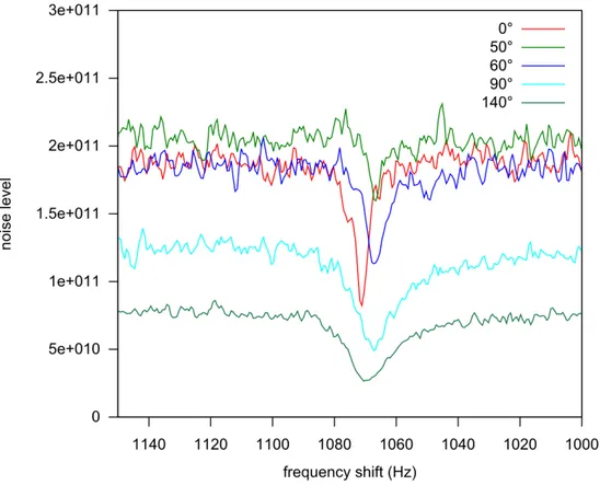
Figure S.3 illustrates how the nuclear spin-noise spectra are affected by the transmission line phase ψ, that is, according to the theoretical developments (Equations 3.10, 3.11 and 3.12) the apparent radiation damping rate 𝜆′𝑟. The linewidths, the depths of the resonance dip as well as the average
noise levels out-of-resonance were affected by the change of this parameter and the induced changed of tuning 𝐶𝑡 and matching 𝐶𝑚capacitors needed for ensuring the observation of SNTO
condition.
Figure S.3. 1H nuclear spin-noise sub-spectra corresponding to CH
3CO resonance of methyl-isopropyl ketone as a function of the transmission phase 𝜓.
In Figure S.4, we report the variation of these four parameters (linewidths, resonance frequencies, noise level at resonance and noise level out-of-resonance) for the whole series of explored transmission phases 𝜓. Firstly one can notice a significant variation of the difference of resonance linewidths as a function of phase 𝜓; the differences were defined by subtracting the full linewidth at half height of 12CH
3CO resonances to that of 13CH3CO resonances. In such a way, variation of field
homogeneity was circumvented; also most of the natural linewidths (𝜆2 contribution) were
cancelled. The apparent radiation damping contributions (𝜆′𝑟 = 𝜋 FWMH) vary from about 0 to 51
8
transmission phase 𝜓 affects these contributions, as predicted by Equation 3.10. In comparison a more restricted variation of the resonance frequencies corresponding to a maximum frequency shift contribution of 19 Hz as a function of the phase shifter angle 𝜓 was detected; it illustrates that with the present electronic system, the SNTO and FSTO conditions can be different but with an extent much more restricted than that observed with a cold probe.4 For the noise levels, when the radiation
damping contributions are at smallest (𝜓 ~ 40°) the average noise level out-of-resonance as well as the noise level at resonance were at maximum. Since uncertainties scale as the amplitudes of the signals in spin-noise experiments,6 it indicates that this configuration (𝜓 ~ 40°) is also the less
favorable for spin-noise determination of NMR parameters. Finally, one can notice that for the four explored parameters their variations as a function of the angle 𝜓 are not a sinusoidal function as discussed in Section I.D of the Supplemental Material.
Figure S.4. Parameters deduced from (a) excitation pulse and (b) spin-noise spectra as a function of the transmission phase 𝜓. (a) Relative variations of the resonance frequencies of CH3CO resonance of methyl-isopropyl ketone referred to that
in the FSTO conditions (squares, the absolute values are directly given as the frequency shift contribution), and of the linewidths (circles, the values are directly given as the radiation damping rate 𝜆′𝑟). (b) Variation of the noise levels in
arbitrary unit, at resonance (triangles) and out-of-resonance (stars) for the different phase values 𝜓. 1. M. A. McCoy and R. R. Ernst, Chem. Phys. Lett. 159 (5,6), 587-593 (1989).
2. D. J. Y. Marion and H. Desvaux, J. Magn. Reson. 193 (1), 153-157 (2008).
3. M. Nausner, J. Schlagnitweit, V. Smrecki, X. Yang, A. Jerschow and N. Müller, J. Magn. Reson. 198 (1), 73-79 (2009).
4. M. T. Pöschko, J. Schlagnitweit, G. Huber, M. Nausner, M. Hornicàkovà, H. Desvaux and N. Müller, ChemPhysChem 15, 3639-3645 (2014).
5. J. Schlagnitweit, S. W. Morgan, M. Nausner, N. Müller and H. Desvaux, ChemPhysChem 13, 482-487 (2012).