HAL Id: inserm-00456967
https://www.hal.inserm.fr/inserm-00456967
Submitted on 16 Feb 2010HAL is a multi-disciplinary open access archive for the deposit and dissemination of sci-entific research documents, whether they are pub-lished or not. The documents may come from teaching and research institutions in France or
L’archive ouverte pluridisciplinaire HAL, est destinée au dépôt et à la diffusion de documents scientifiques de niveau recherche, publiés ou non, émanant des établissements d’enseignement et de recherche français ou étrangers, des laboratoires
Fast FFT-based bioheat transfer equation computation.
Jean-Louis Dillenseger, Simon Esneault
To cite this version:
Jean-Louis Dillenseger, Simon Esneault. Fast FFT-based bioheat transfer equation com-putation.. Computers in Biology and Medicine, Elsevier, 2010, 40 (2), pp.119-123. �10.1016/j.compbiomed.2009.11.008�. �inserm-00456967�
Fast FFT-based bioheat transfer equation
computation
Jean-Louis Dillenseger*,** and Simon Esneault*,**
From:
* INSERM, U642, Rennes, F-35000, France;
** Universit´e de Rennes 1, LTSI, Rennes, F-35000, France; Corresponding author:
Jean-Louis Dillenseger
Laboratoire Traitement du Signal et de l’Image, INSERM U642, Universit´e de Rennes I,
Campus de Beaulieu, 35042 Rennes Cedex, France. tel: +33 (0)2 23 23 55 78 fax: +33 (0)2 23 23 69 17 email: [email protected]
Abstract
This paper describes a modeling method of the tissue temperature evolution over time in hyper or hypothermia. The tissue temperature evolution over time is classically described by Pennes’ bioheat transfer equation which is generally solved by a finite difference method. In this paper we will present a method where the bioheat transfer equation can be algebraically solved after a Fourier transformation over the space coordinates. As an example, we implemented this method for the simulation of a percutaneous high intensity ultrasound hepatocellular carcinoma curative treatment and compared it with the finite difference method and experimental data.
Keywords
Hyperthermia; hypothermia; bioheat transfer equation; BHTE; thermal dose; ultrasound ther-apy.
1
Introduction
The estimation of the temperature evolution in perfused tissues is a central question for the modeling of several therapies like hyperthermia (radiofrequency [1], high intensity ultrasound [2, 3] or laser [4]) or hypothermia cancer treatments [5] or to predict the damage caused by external device i.e. the electromagnetic field of cellular phones [6, 7]. Beside several heating models, the solving of Pennes’ bioheat transfer equation (BHTE) [8] is one of the most popular way to estimate the tissue temperature evolution over time because it simply models not only the temperature diffusion but also takes the perfusion of tissues into account. In this equation, the tissue temperature T evolution over time is governed by:
ρtCt
∂T (x, t)
∂t = kt∇
2T (x, t) + V ρ
bCb(Tb− T (x, t)) + Q(x, t) (1)
where: x is the spatial coordinates, t the time parameter, ρt and Ct refer to tissue density
and specific heat; kt∇2T models the thermal diffusion with kt the thermal conductivity of
tissue; V ρbCb(Tb− T ) models the effect of perfusion where V , ρb, Cb and Tb are respectively the
perfusion rate per unit volume of tissues, the density, the specific heat and the temperature of blood; and Q the rate of the heat per unit volume of tissue produced by the source.
In the case of simple geometry, the BHTE (1) is generally solved by a finite difference [9] method where the temperature Tn+1 at time step n + 1 can be numerically deduced from the temperature Tnat step n. An example of a finite difference modeling in the Cartesian coordinate system can be found in [6]:
Tn+1(x) = Tn(x) + δt ρtCt· ( kt∇2discretTn(x) + V ρbCb(Tb− Tn(x)) + Qn(x) ) (2) ∇2
discretTn(x) is a discrete spatial Laplacian, for example: ∇2discretTn(x, y, z) =
1
∆x2(Tn(x−
1, y, z) + Tn(x + 1, y, z) + Tn(x, y− 1, z) + Tn(x, y + 1, z) + Tn(x, y, z− 1) + Tn(x, y, z + 1)− 6Tn(x, y, z))). δt is the time sampling step which should satisfy the following inequality in order to ensure numerical stability and convergence [6]:
δt≤ 2∆x
2ρ
tCt
V ρbCb∆x2+ 12kt
(3) with ∆x, the spatial sampling step. Generally δt is around 100 ms which leads to a high computation time when we try to estimate the temperature evolution over a long period. Beside the explicit method (2), alternative finite difference methods exist for solving the BHTE e.g. the Crank-Nicholson method, the Du Fort-Frankel algorithm [10] or ADI-FD [11]. These methods
allow larger time sampling steps but are generally not so easy to implement and are more numerically intensive.
However, it is well known that the partial equation of Fourier’s heat conduction problem can be explicitly solved in the case of homogeneous conditions and a regular sampling within the Cartesian Coordinate System after a transformation in the spatial frequency space [12]. But in our knowledge, only little work has been performed to solve the BHTE using this method. In order to evaluate the optimal delivered US power in a temperature control loop, Quesson et al. presented a fast method based on a Fourier Transformation of the bioheat equation [13]. However, this study was performed in 2D and imposed some strong limitations: the tissue is considered as homogeneous with constant parameters and non perfusion occurs (V = 0). In our paper we will extend this idea to solve the BHTE in the spatial frequency space but in 3D and with perfusion.
But in some of the modeling applications the hypothesis of tissue parameter homogeneity can not be stated. This is the case for example for the simulation of the effect of ultrasound interstitial surgery [3] in which the interstitial applicator is cooled by a continuous flow of water maintaining it at a constant temperature or if some main vascular branches acting as cooler are included within the region of interest. Moreover, the final goal of the temperature modeling is usually to assess the thermal damages. For this some non-linear models are used as for example the concept of thermal dose [14] which is quite standard in tumor hyperthermia literature. For each location and history of temperature, the thermal dose is defined as an equivalent time the temperature of reference of 43◦C should be applied to obtain the same thermal damage. It can be computed directly from the temperature map:
D43◦C(x, t) =
t
∑
i=1
R(43−T (x,t))∆t (4)
with R = 0.5 if T > 43◦C and R = 0.25 otherwise. Tissues are considered as irreversibly thermally damaged when D43◦C is greater than a specific time threshold [15]. But in this case the temperature integration over time of (4) can not be analytically solved. In this paper we will present a way to use the explicit BHTE solving in the spatial frequency space to model the temperature evolution and thermal damage in more complex situations. Because the situation is directly related to an application, we will illustrate our idea by the 3D modeling of the thermal coagulation necrosis induced by an interstitial ultrasonic transducer in the liver [3].
2
Methods
2.1 BHTE solving
If we consider that the coefficients ρt, Ct, kt, V , ρb, and Cb remain constant over time, then (1)
can be rewritten as:
A∂T (x, t)
∂t = B∇
2T (x, t) + C(T
b(x)− T (x, t)) + Q(x, t) (5)
where: A = ρtCt, B = ktand C = V ρbCb.
If we take the Fourier transformation of (5) over the space coordinates and use the prop-erty that if F (x) is a differentiable function with Fourier transform F∗(v) (where the symbol
∗ denotes the Fourier Transform and v the spatial frequency coordinates), then the Fourier
transform of its derivative is given by j2πvF∗(v), so:
A∂T ∗(v, t) ∂t =−4π 2v2BT∗(v, t) + C(T∗ b(v)− T∗(v, t)) + Q∗(v, t) (6) 3
The second order partial differential equation over the space domain is translated into an algebraic equation.
If we consider that heat produced by the source Q(x, t) remains constant over time, (6) can be rewritten as a first-order differential equation over the time:
A∂T
∗(v, t)
∂t + (4π
2v2B + C)T∗(v, t) = CT∗
b(v) + Q∗(v) (7)
If Tinit∗ (v) is the Fourier transform of the initial temperature map at t = 0, an analytical solution can be found for (7):
T∗(v, t) = Tinit∗ (v) exp−(4π2v2B+C)tA +CT ∗ b(v) + Q∗(v) 4π2v2B + C ( 1− exp−(4π2v2B+C)tA ) (8)
2.2 Implementation and boundary conditions
As stated in the introduction, the implementation of a solution is directly related to an ap-plication. In our case, we wish to model the therapeutical effect of an interstitial ultrasound surgery device [16]. This device is composed of a small (3 mm x 10 mm) planar ultrasonic mono-element transducer encapsulated in a ∅ 4 mm cylindrical interstitial applicator which is set within the tumor under ultrasound image guidance. The front transducer face is cooled by a continuous degassed water flow maintained at a constant temperature. The therapy consists in a sequence of exposures. Some properties of this ultrasound therapy and boundary conditions must be taken into account for the implementation:
• The thermal dose (4) is an integration. The temperature must be computed at several
time steps ∆t.
• The temperature of the cooling water serves as an iso-thermal boundary condition. But
this condition cannot be described explicitly in (8). However, this condition can be incor-porate in the model by the following iterative process:
1. With (8), compute explicitly T (x, ∆t), the temperature map at a specific time step ∆t.
2. In T (x, ∆t), modify the temperature for the x within the interstitial device to the temperature of the cooling water.
3. The modified T (x, ∆t) serves then as a new initial temperature Tinit(x) map (8) in
order to compute the temperature map at the next time step ∆t.
• As ebullition is not considered in the present model and for avoiding unrealistic
temper-atures; a threshold must ensure that the temperature could never exceed 100◦C. This threshold is incorporated in the model using the iterative process described previously.
• In [3, 17], we have shown that for more realistic modeling, the acoustic power Q is
tem-perature dependent and so does not remain constant over time. However, because the temperature evolution over time is relatively slow, we can consider that Q remains con-stant during a time step ∆t. So Q needs only to be actualized after each ∆t and can be incorporated in the model using the iterative process described previously.
The implemented algorithm can so be summarized by:
1. Initialization. Tb(x) is build by setting the temperature within the interstitial device to
the temperature of the cooling water and to 37◦C elsewhere. Tb∗(v) is then computed. At
2. Temperature map estimation. At t = t + ∆t, T∗(v, ∆t) is computed using (8) in order to estimate T (x, ∆t).
3. Boundary effects and thermal dose. T (x, ∆t) is modified in order to take the cooling water effect and temperature threshold into account. The thermal dose (4) is updated.
4. Acoustical power. Q(x) can be computed by taking new shooting parameters and/or the new temperature map T (x, ∆t) into account.
5. Next iteration initialization. The new Tinit∗ (v) is estimated from the Fourier Transform of T (x, ∆t) modified at step 3. The new Q∗(v) is also computed. t is incremented by ∆t and a new iteration can be computed from step 2.
3
Results and Discussion
3.1 Simulation context
For evaluation purpose, we choose to simulate a real in vivo experiment described in [16]. A 10.7 MHz therapeutic ultrasound device was positioned inside the liver of pigs, away from large blood vessels. This animal experimentation was approved by a veterinarian ethics committee. The exposure conditions were set to: 14 W/cm2 for the intensity measured by a force balance at the surface of the applicator; 37◦C for the transducer cooling water temperature and 20 s for the duration of the exposure. Four thermocouples were introduced inside the liver on the acoustic axis of the transducer right at the end of the 20 s-long exposure. The maximum increase of temperature was measured at four different positions: 2.5, 5, 7.5 and 10 mm from the applicator surface. During this in vivo experiment, 10 lesions were carried out. The means and the standard deviations of the 10 peak temperatures measured at each position are reported on Fig. 2 as error bars.
3.2 Method implementation
The simulation is performed within a 256× 256 × 64 volume grid with a sampling step ∆x of 0.4 mm on each direction (which corresponds to a 102 mm× 102 mm × 25.4 mm simulation volume). The simulated applicator is set in the middle of this volume.
In the case of high intensity ultrasound therapy, Q is an acoustical power given by Q =
βf p2/ρtc where β is the absorption coefficient of ultrasound in tissues which depends on the
tissue temperature [18]; f , the ultrasound frequency; c, the ultrasound velocity and p, the pressure delivered by the ultrasound device. In our simulation, p is computed using a discrete Rayleigh integral [17] and considered as invariant over time. On the contrary, the temperature dependent absorption coefficient map β(x, t) and so the acoustical power Q(x, t) are updated after each time step ∆t. The used tissue acoustical and thermal properties were found in the literature [19, 20, 21] and set to: ρt = 1050 kg· m−3, Ct = 3639 J· kg−1·◦C−1, kt =
0.56 W· m−1·◦C−1, V ρb = 30kg· m−3· s−1 and Cb = 3825 J· kg−1·◦C−1.
This simulation has been developed using the C++ language and implemented on a standard PC (Xeon E5410-Quad Core CPU 2.33 GHz, 4 Go RAM). Fourier transforms were computed using the FFTW library [22].
As an example, Fig. 1 presents on the upper line the simulated temperature map computed at t = 20 s and on the lower line the corresponding simulated necrotic volume (in white on the figure) on two orthogonal cut planes (Fig. 1-left: axial cut plane perpendicular to the applicator axis; Fig. 1-right: sagittal cut plane along the applicator axis).
Fig. 2 compares the real temperatures measured on the in-vivo experimental validation at the four different positions [16] and the temperature curves obtained by our simulation method. The temperature curve obtained by our approach seems to match with the experimental data.
Figure 1: Simulated temperature map (upper line) and necrotic volume (lower line). Left: cut plane perpendicular to the applicator axis. Right: cut plane along the applicator axis. The temperature color scale goes from black (37◦C) to white (66◦C).
The effect of the transducer cooling water can also be noticed near the applicator surface (on the left of the curve).
0 5 10 15 20 25 30 35 40 35 40 45 50 55 60 65 70 75
Distance from the applicator axis (mm)
Temperature (°C)
In vivo measurements (means and stdv) FFT based method
finite difference based method
Figure 2: Comparison between the experimental in-vivo temperature measurements and the simulated temperatures obtained with the FFT based method and the finite difference based method.
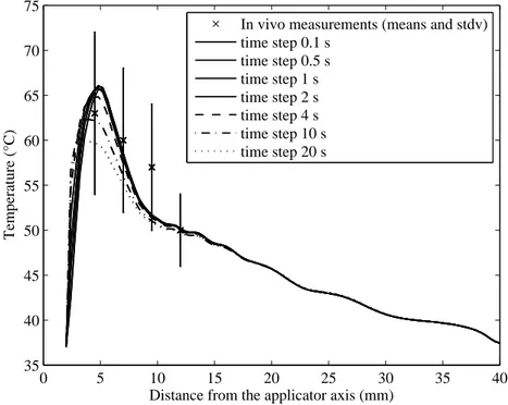
3.3 Time step influence
In section 2.2, it has been shown that the choice of the time step ∆t is crucial for the balance between computation speed and accuracy of the model. In order to evaluate the influence of ∆t, several BHTEs were computed with ∆t varying from 0.1 s to 20 s.
Fig. 3 presents the temperature curves along the axis perpendicular to the transducer surface and obtained when computing the BHTE with the several ∆t. The curves are very similar when ∆t≤ 2 s. Only the temperature profiles near the applicator surface are a bit different. This is due to the different cooling water iso-thermal boundary condition refreshment rates. However, the curves are relatively different when ∆t > 2 s. In these cases, the low refreshment rate affects not only the cooling water iso-thermal boundary condition but also the estimation of the acoustical power Q. This is confirmed by error measurements: the curve computed with ∆t = 0.1 s is considered as reference; the Mean Squared Errors between the other curves and the reference curve are reported on Table 1. The computation times of the 20 s sequence simulation (computed with the non parallel FFTW) are also reported on Table 1.
0 5 10 15 20 25 30 35 40 35 40 45 50 55 60 65 70 75
Distance from the applicator axis (mm)
Temperature (°C)
In vivo measurements (means and stdv) time step 0.1 s time step 0.5 s time step 1 s time step 2 s time step 4 s time step 10 s time step 20 s
Figure 3: Comparison between the simulated temperatures obtained with ∆t varying from 0.1 s to 20 s.
Table 1: Temperature field estimation Mean Squared Errors and computation time vs. time step
∆t (s) 0.1 0.5 1 2 4 10 20
MSE (◦C2) 0 0.23 0.75 1.75 3.06 4.61 5.41
Comp. time (s) 860 180 91 53 23 8 3
3.4 Comparison with the finite difference method
We also implemented the finite difference scheme using (2). The tissue parameter homogeneity hypotheses (ρt, Ct, kt, V , ρb, and Cbremain constant over time) and acoustic power computation
were similar to these of the FFT-based method. The time sampling step which should satisfy the inequality (3) is for our spatial sampling steps: δt≤ 180 ms. The comparison framework of both BHTE solving methods is:
• the FFT-based computation method used a ∆t = 2 s;
• the finite difference method used a δt = 0.1 s. Q is actualized after the same ∆t = 2 s as
for the FFT-based computation method.
The temperature maps obtained by both methods were almost similar (Fig. 2). However, if we compare closer both methods, the FFT-based one shows some limitations. Because of the classical FFT, the temperature equation can only be solved on equidistant grid steps with no possibility to locally adapt the space sampling. Other limitations are inherent to the analytical first-order differential equation solving (8) which needs a linear Bioheat equation. Constant parameters can affect the accuracy of the model on two aspects:
• Only hyperthermia in relatively homogeneous tissues can be simulated. But this is the
case of our interstitial ultrasound therapy which is locate in a small area.
• The tissue parameters vary with the temperature and the tissue damage stage [23, 24].
Some of the parameters variations can be integrated in (8) by updating Q as for example the attenuation and absorption coefficients of ultrasound in tissues. But the temperature and damage dependence of the other parameters of (1), e.g. the perfusion rate [23], cannot be integrated in our scheme and must be assumed as constant. However, for simplicity and computation speed, many of the hyperthermia models have assumed constant parameters independent of temperature. Moreover, the accuracy of the model is depending on a accurate estimation of the patient specific tissue acoustical and thermal parameters. The parameters found in the literature show a great variability among one paper to another. This variability can also explain the distribution of the real temperature measurements reported as error bars on Fig. 2. Some more evaluation should be performed to compare the accuracy gain provided by the non linear Bioheat equation relative to the imprecision due to parameters dispersion.
The computation times of the sequence simulation were 53 s and 62 s for respectively the FFT-based and the finite difference method. Our starting hypothesis was that the BHTE alge-braic solving using the FFT-based method should bring good computation time performances. However, its performance is not as good as expected. This is mainly due to the FFTs which are computation time consuming: for each ∆t iteration two direct FFTs (Tinit∗ (v) and Q∗(v)) and one inverse FFT (T (x, ∆t)) must be computed.
In our specific case, the temperature evolution must be computed with a relatively short sampling interval ∆t of around 2 s because of the thermal dose integration, the cooling water iso-thermal boundary condition and the fact that the acoustical power Q is temperature dependent (and so time dependent). For this reason, the algebraically BHTE solving did not provide the expected performance. However, some gain can be obtained using specialized signal processing or mathematical libraries or vector, parallel or graphic processors in order to accelerate the Fourier Transforms computation. For example, we used the FFTW parallelization capability of our 4 processors computer, the computation times is decreased to 31 s. FFTW can also run on Graphics Processing Units using for example NVIDIA’s CUDA environment1. On a NVIDIA Quadro FX 4600 graphic card the computation time is decreased to 13 s including the data transfer time. These two implementations have been easily realized by just modifying some little high level C++ code. At the other hand, the classical finite difference approach can also take benefit from an implementation on GPU implementation (e.g. Laplacian filtering) or on distributed architectures [25]. However, this later implementation requires specialized architectures and algorithms.
1
4
Conclusion
A method simulating the tissue temperature evolution over time was described. This method solves algebraically the bioheat transfer equation after a Fourier transformation over the space coordinates. However, the integrative nature of the thermal dose, the isothermal conditions and/or the temperature dependence of the simulation constrained us to decompose the entire analytical temperature evolution computation into several smaller time intervals. The tempera-ture computation at these intermediate time steps makes the FFT-based method less efficient in terms of computation time. Notwithstanding this method becomes interesting again using spe-cialized processing libraries or processors or for solving problems with conditions less dependent on the time evolution.
Acknowledgements
This work is part of the French SUTI project supported by an ANR Grant (ANR05RNTS01106).
References
[1] Enrique Berjano. Theoretical modeling for radiofrequency ablation: state-of-the-art and challenges for the future. BioMedical Engineering OnLine, 5(1):24 pages, 2006.
[2] C. Lafon, F. Prat, J. Y. Chapelon, F. Gorry, J. Margonari, Y. Theillere, and D. Cathig-nol. Cylindrical thermal coagulation necrosis using an interstitial applicator with a plane ultrasonic transducer: in vitro and in vivo experiments versus computer simulations. Int
J Hyperthermia, 16(6):508–22, 2000.
[3] C. Garnier, C. Lafon, and J.-L. Dillenseger. 3D modeling of the thermal coagulation necrosis induced by an interstitial ultrasonic transducer. IEEE Trans Biomed Eng, 55(2):833–7, 2008.
[4] J. Zhou, J. K. Chen, and Y. Zhang. Theoretical analysis of thermal damage in biological tissues caused by laser irradiation. Mol Cell Biomech, 4(1):27–39, 2007.
[5] A. A. Konstas, M. A. Neimark, A. F. Laine, and J. Pile-Spellman. A theoretical model of selective cooling using intracarotid cold saline infusion in the human brain. J Appl Physiol, 102(4):1329–40, 2007.
[6] J. Wang and O. Fujiwarea. FDTD computation of temperature rise in the human head for portable telephones. IEEE Trans Microwave Theory Tech, 47(8):1528–34, 1999.
[7] E. Neufeld, N. Chavannes, T. Samaras, and N. Kuster. Novel conformal technique to reduce staircasing artifacts at material boundaries for FDTD modeling of the bioheat equation.
Phys Med Biol, 52(15):4371–81, 2007.
[8] H. H. Pennes. Analysis of tissue and arterial blood temperatures in the resting human forearm. 1948. J Appl Physiol, 85(1):5–34, 1998.
[9] J.C. Chato, M. Gautherie, K.D. Paulsen, and R.B. Roemer. Fundamentals of bioheat transfer. In M. Gautherie, editor, Thermal dosimetry and treatment planning, pages 1–56. Springer, Berlin, 1990.
[10] F. Fanjul-V´elez, O. G. Romanov, and J. L. Arce-Diego. Efficient 3D numerical approach for temperature prediction in laser irradiated biological tissues. Comput. Biol. Med., 39(9):810– 7, 2009.
[11] S. Pisa, M. Cavagnaro, E. Piuzzi, P. Bernardi, and J. C. Lin. Power density and tempera-ture distributions produced by interstitial arrays of sleeved-slot antennas for hyperthermic cancer therapy. IEEE Trans Microwave Theory Tech, 51(12):2418–26, 2003.
[12] M. N. ¨Ozisik. Boundary value problems of heat conduction. Dover publications, Mineola, N.Y., 1989.
[13] B. Quesson, F. Vimeux, R. Salomir, J. A. de Zwart, and C. T. Moonen. Automatic control of hyperthermic therapy based on real-time Fourier analysis of MR temperature maps.
Magn Reson Med, 47(6):1065–72, 2002.
[14] S. A. Sapareto and W. C. Dewey. Thermal dose determination in cancer therapy. Int J
Radiat Oncol Biol Phys, 10(6):787–800, 1984.
[15] S. J. Graham, L. Chen, M. Leitch, R. D. Peters, M. J. Bronskill, F. S. Foster, R. M. Henkelman, and D. B. Plewes. Quantifying tissue damage due to focused ultrasound heating observed by MRI. Magn Reson Med, 41(2):321–8, 1999.
[16] C. Lafon, J. Y. Chapelon, F. Prat, F. Gorry, J. Margonari, Y. Theillere, and D. Cathig-nol. Design and preliminary results of an ultrasound applicator for interstitial thermal coagulation. Ultrasound Med Biol, 24(1):113–22, 1998.
[17] J.-L. Dillenseger and C. Garnier. Acoustical power computation acceleration techniques for the planning of ultrasound therapy. In 5th IEEE International Symposium on Biomedical
Imaging (ISBI’08), pages 1203–6, Paris, 2008.
[18] C. W. Connor and K. Hynynen. Bio-acoustic thermal lensing and nonlinear propagation in focused ultrasound surgery using large focal spots: a parametric study. Phys Med Biol, 47(11):1911–28, 2002.
[19] F. Dunn and W. D. O’Brien. Ultrasonic biophysics, volume 7 of Benchmark papers in
acoustics. Dowden-Hutchinson & Ross Inc., Stroudsburg (Pennsylvania), 1976.
[20] Task group report of the european society for hypermermic oncology. Treatment planning
and modeling in hyperthermia. Tor Vergata Medical Physic Monograph Series. University
of Rome, 1992.
[21] P Bioulac-Sage, B. Le Bail, and C. Balaudaud. Histologie du foie et des voies biliaires. In J.P. Benhamou, J. Bircher, N. McIntyre, M. Rizetto, and J. Rodes, editors, H´epathologie clinique, pages 12–20. Med. sciences/Flammarion, Paris, 1993.
[22] M. Frigo and S. G. Johnson. The design and implementation of FFTW3. Proc IEEE, 93(2):216–31, 2005.
[23] Chang W. Song, Anna Lokshina, Juong G. Rhee, Marsha Patten, and Seymour H. Levitt. Implication of blood flow in hyperthermic treatment of tumors. IEEE Trans Biomed Eng, (1):9–16, 1984.
[24] C. A. Damianou, N. T. Sanghvi, F. J. Fry, and R. Maass-Moreno. Dependence of ultrasonic attenuation and absorption in dog soft tissues on temperature and thermal dose. J Acoust
Soc Am, 102(1):628–34, 1997.
[25] O. Schenk, M. Manguoglu, A. Sameh, M. Christian, and M. Sathe. Parallel scalable PDE-constrained optimization: antenna identification in hyperthermia cancer treatment planning. Computer Science - Research and Development, 23(3):177–83, 2009.