Climate impact metrics for energy technology evaluation

Climate Impact Metrics for Energy Technology Evaluation by

Morgan R. Edwards B.S. Environmental Science

University of North Carolina at Chapel Hill, 2010

SUBMITTED TO THE ENGINEERING SYSTEMS DIVISION IN PARTIAL FULFILLMENT OF THE REQUIREMENTS FOR THE DEGREE OF

MASTER OF SCIENCE IN TECHNOLOGY AND POLICY

AT THE

MASSACHUSETTS INSTITUTE OF TECHNOLOGY JUNE 2013

©

Signature of Author:

MCHNES

JUN 12 2013

LBRARIES

Engieering Systems Division May 10, 2013

Certified by:

Jessika E. Trancik Assistant Professor of Engineering Systems Thesis Supervisor

Accepted by:

Professor of Aeronautics

(

Climate Impact Metrics for Energy Technology Evaluation

Morgan R. Edwards

Submitted to the Engineering Systems Division on May 10, 2013 in partial fulfillment of the requirements of the degree of

Master of Science in Technology and Policy

ABSTRACT

The climate change mitigation potential of energy technologies depends on how their lifecycle greenhouse gas emissions compare to global climate stabilization goals. Current methods for comparing technologies, which assess impacts over an arbitrary, fixed time hori-zon, do not acknowledge the critical link between technology choices and climate dynamics. In this thesis, I ask how we can use information about the temporal characteristics of green-house gases to design new metrics for comparing energy technologies.

I propose two new metrics: the Cumulative Climate Impact (CCI) and Instantaneous

Climate Impact (ICI). These metrics use limited information about the climate system, such as the year when stabilization occurs, to calculate tradeoffs between greenhouse gases, and hence the technologies that emit these gases. The CCI and ICI represent a middle ground between current metrics and commonly-proposed alternatives, in terms of their level of complexity and information requirements.

I apply the CCI and ICI to evaluate the climate change mitigation potential of energy technologies in the transportation sector, with a focus on alternative fuels. I highlight key policy debates about the role of (a) natural gas as a "bridge" to a low carbon energy future and (b) third generation biofuels as a long-term energy solution. New metrics shed light on critical timing-related questions that current metrics gloss over. If natural gas is a bridge fuel, how long is this bridge? If algae biofuels are not commercially viable for the next twenty years, can they still provide a significant climate benefit?

I simulate technology decisions using new metrics, and existing metrics like the Global

Warming Potential (GWP), identifying the conditions where new metrics improve on existing methods as well as the conditions under which new metrics fail. I show that metrics of intermediate complexity, such as the CCI and ICI, provide a simple, reliable, and policy-relevant approach to technology evaluation and capture key features of the future climate system. I extend these insights to energy technologies in the electricity sector as well as a variety of environmental impact categories.

Thesis Supervisor: Jessika E. Trancik

Acknowledgements

I owe a debt of gratitude to a number of individuals for their support and encouragement

over the past two years. I would especially like to thank:

" Jessika Trancik. For being a wonderful teacher, mentor, and friend. The perspective

and dedication you bring to research is invaluable.

" James McNerney and Mandira Roy. I have learned so much working with you on this

project. This thesis would not exist without you.

* The rest of the Trancik Lab - Michael Chang, Dan Cross-Call, Goksin Kavlak, and Hamed Ghoddusi. Thank you for your feedback and your company in E-40.

" My thesis-writing group - Amanda Giang, Ingrid Bonde-Akerlind, and Alice Chao. You made working on my thesis fun (most of the time).

" John Hess. For hearing about this research in its endless iterations and always

provid-ing encouragement and helpful suggestions.

" My friends in TPP and ESD. You have defined my experience here at MIT and made

Cambridge, MA my home.

* My family - Dad, Mom, Erika, and Alex. I love you all so much.

This research described in this thesis was conducted as part of a collaborative project which has resulted in two papers in preparation [24, 25]. This project was supported by a Lemelson Engineering Presidential Fellowship and a grant from the New England University Trans-portation Center.

Contents

2.1.1 Energy Options for Transportation . . . . 14

2.1.2 Technical and Economic Challenges . . . . 16

2.1.3 _{Climate and Environmental Impacts . . . . 18}

2.2 Climate Metrics and Policy . . . . 22

2.2.1 Greenhouse Gases and Climate . . . . 22

2.2.2 _{History of Climate Metrics . . . . 25}

2.2.3 Questions for Designing Metrics . . . .. . . . . 27

2.2.4 Review of Alternative Metrics . . . . 30

2.2.5 _{Climate Metrics Going Forward . . . . 32}

3 Methods ₃₃ 3.1 _{Emissions Data . . . . 33} 3.2 _{Climate Scenarios . . . . 34} 3.3 Metric Design . . . . 43 3.4 Metric Testing. . . . . 44 4 Results 49 4.1 Classifying Climate Metrics . . . . 49

4.2 Simple Static Metrics . . . . 51

4.4.1 Metric Design . . . . 57

4.4.2 Metric Testing . . . . 59

4.4.2.1 Climate Impacts . . . . 59

4.4.2.2 Technology Evaluation . . . . 62

5 Discussion 66 5.1 Metrics in Transportation Policy. . . . . 66

5.1.1 Current Policies . . . . 66

5.1.2 Role for New Metrics . . . . 70

5.2 Challenges for Metrics in Policy . . . . 72

5.2.1 Science Policy Analysis . . . . 72

5.2.2 Stakeholder Analysis . . . . 74

5.3 Insights for Other Policy Areas . . . . 75

5.3.1 Electricity Technology Policy . . . . 75

5.3.2 Other Environmental Policies . . . . 77

6 Conclusion 80 A Derivations 82 Bibliography . . . . 87

Figures, Tables, and Abbreviations

List of Figures

Energy and Petroleum Demand in Transportation Environmental Impacts of Transportation Fuels Changes to the Earth's Radiative Forcing Budget Radiative Forcing Trajectories of Greenhouse Gases The Emissions-to-Climate Impacts Causal Chain. .

. . . . 15

. . . . 20

. . . . 24

. . . . 25

. . . . 28

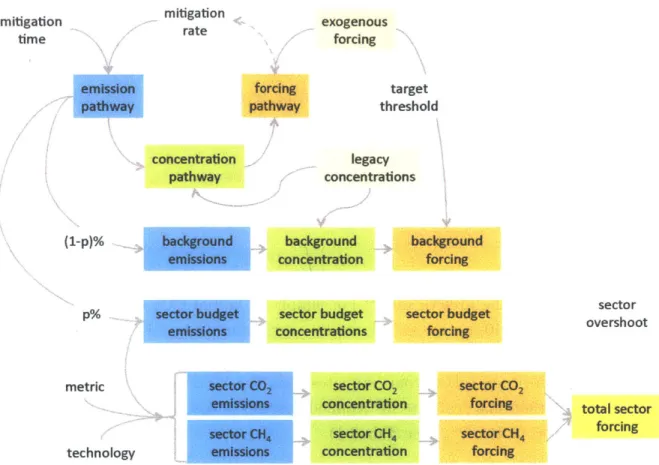
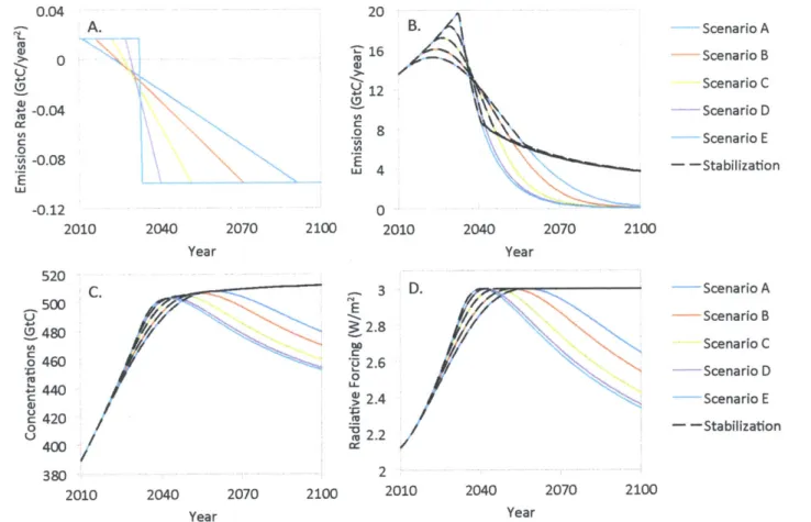
Schematic of the Metric Design and Testing Process . . . . Greenhouse Gas Emissions and Emissions Rate . . . . Greenhouse Gas Decay Rate and Concentrations . . . . Major Components of Radiative Forcing Pathways . . . . . Emission, Concentration, and Radiative Forcing Scenarios Sector Radiative Forcing Budget Calculation . . . . Metric Complexity and Information Availability . . . . Transportation Fuel Comparisons with the GWP... Sector-Specific Impacts from Using the GWP... Global Climate Impacts from Using the GWP . . . . Illustration of CCI and ICI Design Process . . . . Global Climate Impacts from Using the CCI and ICI . . . Overshoot of Thresholds with the ICI and GWP . . . . Sector-Specific Results from Using the ICI and CCI . . . . Transportation Fuel Comparisons with the CCI and ICI . . 36 37 39 . . . 41 42 47 2.1 2.2 2.3 2.4 2.5 3.1 3.2 3.3 3.4 3.5 3.6 4.1 4.2 4.3 4.4 4.5 4.6 4.7 4.8 4.9

List of Tables

. . . . 51 . . . . 52 . . . . 53 . . . . 54 . . . . 58 . . . . 60 . . . . 61 . . . . 63 . . . . 64

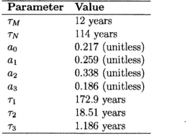
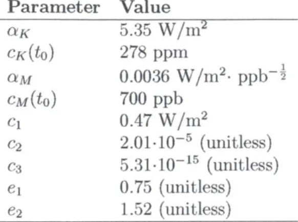
3-2 Parameter Values for Concentration Calculations . . . . 38 3-3 Parameter Values for Radiative Forcing Calculations . . . . 41

List of Abbreviations

"

" CCI: Cumulative Climate Impact " CNG: Compressed Natural Gas

" DAI: Dangerous Anthropogenic Interference " E85: 85% Ethanol Blend with Gasoline " GCP: Global Cost Potential

" GDP: Global Damage Potential " GTP: Global Temperature Potential " GWP: Global Warming Potential " ICI: Instantaneous Climate Impact

Chapter 1

Introduction

1.1

Motivation

World energy demand is expected to increase by 50% over the next 25 years, necessitating major growth in new energy infrastructure [28]. Given the scale of the investments required and the potential for devastating environmental impacts, designing and evaluating sustain-able energy technologies presents a critical engineering challenge. Energy technologies carry a range of environmental impacts. However, these impacts are difficult to assess because they depend on aggregate characteristics of the environmental system - including green-house gas concentrations, air pollution levels, and cumulative resource consumption - and the proximity to large-scale climate change, human health, and natural resource thresholds. As a result, a technology's impact can vary dramatically over time and across locations, depending on the longevity and distribution of its life cycle emissions and resource use, and the timing of thresholds. Humanity is rapidly approaching these critical thresholds [92]. Thus, understanding the dynamic interactions between energy technologies and an evolving environmental system is essential.

This thesis focuses on the climate impacts of alternative transportation fuels. Trans-portation represents 19% of energy consumption and 23% of energy-related carbon dioxide

(C02) emissions worldwide, and these emissions are expected to increase by more than 80%

in the next 35 years [49]. This rapid growth trajectory suggests that any reasonable policy to reduce the climate and environmental impacts of energy consumption must include a plan for substantial changes to the business-as-usual transportation system. Vehicle efficiency improvements and reductions in travel demand can contribute to this goal. However, these energy-saving solutions all have fundamental limits in their ability to reduce total emissions (see Eq. 1.1).1 Ultimately, major reductions in emissions - to compensate for increasing

'iEq. 1.1 is called the Kaya identity [41, 86]. It is a variant on the popular IPAT identity, which represents a generic environmental impact (I) as the product of population (P), affluence (A), and technology (T) [26].

population and wealth per capita - can only be achieved through changes in the emissions intensity of energy technologies. Thus, alternative fuels and other energy sources will be critical for transforming the transportation sector.

. Wealth Energy Emissions

Em'issions =Population x x x(1)

Population Wealth Energy

Evaluating the impacts of alternative transportation fuels is challenging. Fuels emit a variety of pollutants, and these pollutants have different lifetimes and potencies. As a result, comparisons of fuels change depending on the time horizon over which impacts are evaluated. In addition, policies that impact fuel technology choices exist at many levels of aggregation, and environmental goals are incorporated into these policies in different ways. Policy options range from local and regional transportation planning to national technology mandates and research portfolios to global emissions treaties. Previous research on transportation fuels is equally fragmented, focusing on evaluating specific fuels across multiple criteria [7], comparing multiple fuels against a single criterion [58], quantifying changing environmental constraints [95], or performing location-specific impact assessments

[72]. However, the full meaning of these strands of research is not readily apparent in isolation. We must draw on all of these insights to develop metrics that allow policymakers at multiple decision-making scales to create policies whose collective outcomes meet climate change mitigation goals.

1.2

Research Objectives

In this thesis, I propose new metrics for evaluating the climate change mitigation potential of energy technologies, which capture the effects of a changing climate system on the dy-namics of technology performance [24, 25]. These metrics have a wide variety of potential applications. They can quantify tradeoffs between new technology designs in the laboratory, prioritize among competing technologies for long-term infrastructure planning, and guide policymakers in setting technology performance targets. I argue that metrics should link individual technology decisions, or groups of connected decisions, to their collective envi-ronmental impacts at local, regional, and global scales. At the same time, these metrics must acknowledge uncertainty in the future state of the environmental system, and allow this uncertainty to be reflected to decision-makers. Equally important, metrics must be ap-propriate for the technology policy context in which they will be used, balancing simplicity and transparency with a more comprehensive representation of environmental impacts. Other impact-specific identities can be developed in the same vein as the Kaya identity, for example to study the drivers of natural resource consumption or local and regional air pollution.

I apply these new metrics to study the climate impacts of alternative transportation fuels.

Since fuels vary widely in the composition of greenhouse gases they emit, and these gases have different heat trapping abilities and atmospheric lifetimes, we expect a fuel's climate impact will depend on the timing and composition of its emissions and their relation to changing climate constraints. This fact is often neglected in policy discussions. Natural gas, for instance, has been proposed as a "bridge" to a low-carbon future [73]. While natural gas has lower CO₂ emissions than coal for electricity or gasoline for transportation, it has substantial non-CO2 emissions [5]. Given these differences, it is unclear how to value natural

gas in a climate change mitigation portfolio. Is it a viable bridging technology, and if so how long is the bridge? How do energy technologies with high non-CO2 emissions compare to

those that emit primarily C0 2? To answer these critical policy questions, a new

technology-focused approach to valuing the impacts of greenhouse gases is needed.

My central research question is - how can we evaluate the environmental impacts of en-ergy technologies in the context of a changing environmental system? I explore this question in depth for the case of alternative transportation fuels and climate change and use this ex-ample to identify general challenges and opportunities for developing environmental metrics, which can be applied to a wide variety of technologies and impacts. My general research question can be broken down further as follows:

1. How does the climate impact of a greenhouse gas depend on the timing of the emission

and the state of the climate system? How do emissions decisions using current metrics, which do not reflect climate system dynamics, deviate from intended climate outcomes? 2. Can we use information about the temporal characteristics of greenhouse gases to

design new metrics for comparing alternative fuels? Under what conditions do these new metrics improve on current metrics, and under what conditions do they fail?

3. How do alternative fuels compare, and how does this comparison depend on climate

conditions and mitigation goals? Can we develop general insights, such as preferred pathways for technological change, that are robust to a range of future conditions? 4. How do social, political, and economic factors influence the tradeoffs between simple

and complex metrics, and their relationship to broader climate goals? Under what conditions might different levels of complexity be preferred?

Answers to these four questions form the argument of my thesis. On the one hand, I argue that the context of use matters for comparing energy technologies, and that metrics that incorporate changing environmental constraints can improve technology choices to meet climate change mitigation goals. On the other hand, I argue that the usefulness of metrics that are tightly bound to detailed features of the climate system is limited by uncertainties

in how this system will change over time, as well as political barriers to implementing and revising complex metrics. This suggests that metrics of intermediate complexity, which recognize the importance of context, limitations in scientific understanding, and the realities of the political process, provide a possible way forward for evaluating the climate change mitigation potential of alternative transportation fuels, and the environmental impacts of energy technologies more broadly.

1.3

Thesis Structure

Following this introduction, Ch. 2 Background describes the specific energy technology and environmental impact categories that I focus on in this thesis: alternative transportation fuels and climate change. Sec. 2.1 reviews energy options for transportation, highlighting the technical, economic, and environmental challenges with conventional and alternative fuels, as well as other energy sources. Sec. 2.2 describes the role of greenhouse gases in climate change, discussing historical efforts to compare greenhouse gases and options for comparing gases for technology and climate policy. Ch. 3 Methods describes the approach I developed to answer the research questions posed in this introduction, which uses a simple climate model (Sec. 3.2) to develop and test new climate metrics (Sec. 3.3 and Sec. 3.4), and uses these metrics along with emissions data (Sec. 3.1) to compare alternative transportation fuel technologies (Sec. 3.5).

Ch. 4 Results introduces a new approach to classifying climate metrics (Sec. 4.1),

first providing insights from evaluating existing metrics (Sec. 4.2 and Sec. 4.3) and then proposing and testing a new class of metrics (Sec. 4.4). I emphasize the role of climate metrics in technology evaluation, illustrating what we learn about technologies when we apply different metrics. Ch. 5 Discussion assesses how climate metrics relate to climate and technology policy for transportation. Sec. 5.1 reviews current transportation policies and discusses the role new climate metrics could play in these policies. Sec. 5.2 describes the challenges in bringing new metrics into technology policymaking and identifies promising policy areas for introducing new metrics. Sec. 5.3 then extends the insights developed in this thesis to other technology evaluation and environmental challenges. Ch. 6 Conclusion summarizes the key outcomes of this thesis and the answers to the four research questions posed in the introduction.

Chapter 2

Background

In this chapter, I review energy options for transportation and their technical, economic, and environmental challenges (Sec. 2.1). I then discuss climate metrics and policy, focusing on metrics for comparing the climate impacts of greenhouse gases and their application to tech-nology evaluation (Sec. 2.2). In Ch. 3 Methods, and Ch. 4 Results, I focus in depth on the specific case of alternative transportation fuels and climate change. Narrowing the scope allows me to drill down into the technology and policy details of the problem and explore how these details impact the usefulness and appropriateness of new types of environmental performance metrics. At the same time, the more general background provided in this chap-ter places the insights from these lachap-ter chapchap-ters within a broader technical, economic, and environmental context.

2.1

Energy and Transportation

2.1.1

Energy Options for Transportation

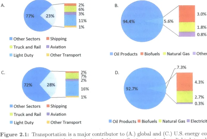
The transportation sector is a major contributor to energy consumption and therefore also climate change and other environmental impacts. Currently, transportation is overwhelm-ingly dominated by petroleum, which supplies 95% of transportation energy demand world-wide. Other energy sources, including natural gas fuels (primarily CNG and LNG, and to a lesser extent methanol), biofuels from a variety of source crops (including bioethanol and biodiesel), and electricity (using plug-in hybrid and battery electric vehicles), represent only

5% of total energy use globally (see Fig. 2.1). However, these fuels are expected to play a

more significant role in the future, partially due to their potential to mitigate climate change and other environmental impacts. The U.S., Europe, Brazil, and other countries are aggres-sively promoting biofuel production and use, and one estimate - albeit uncertain - suggests that 27% of transportation energy could be supplied by biofuels by 2050 [49]. Natural gas is

also being discussed as a serious contender, particularly in the U.S., where recent discoveries of large unconventional gas reserves are making the infrastructure investment required to shift to natural gas more economical. Electrification is also becoming more feasible with

improvements in batteries and other related vehicle technologies.

A.

Other Sectors Truck and Rail Light Duty ~~ on2% 6% 23% 3% 11% 1% * Shipping F Aviation Other Transport C. 28% Other Sectors Truck and Rail Light Duty 2% 7% 2% 16% 1% * Shipping U Aviation Other Transport B. E 3.0% 5.6% 1.8% 0.8%

L Oil Products U Biofuels Natural Gas 99 Other

7.3% D.

4.3%

2.7% 0.3%

Oil Products U Biofuels Natural Gas 0 Electricity

Figure 2.1: Transportation is a major contributor to (A.) global and (C.) U.S. energy

con-sumption, with the majority of this contribution coming from light duty vehi-cles and trucks. Transport energy supply is heavily dominated by petroleum both (B.) globally and (D.) in the U.S., although both show some contributions from biofuels, natural gas, and other sources. Data source: [28, 48].

However, in spite of the apparent optimism surrounding alternative energy, there are serious obstacles to fueling a significant share of transportation demand with non-petroleum sources. Petroleum fuels such as gasoline and diesel perform well across a wide range of criteria: they are energy-dense, easy to transport and store, and relatively low cost. There have also been enormous investments in optimizing petroleum vehicles as well as petroleum extraction, refinement, and distribution [49]. These conditions suggest that climate change mitigation may be more difficult for the transportation sector than the electricity sector. They also imply a critical role for other mitigation options, including improved energy ef-ficiency, transportation mode switching, and reductions in travel demand. However, given

measures, while necessary, are likely to be insufficient on their own. This is particularly true in light of growing populations and increased mobility in developing countries. A low carbon energy source must be part of the solution.

2.1.2

Technical and Economic Challenges

Large-scale deployment of alternative transportation energy sources presents serious techni-cal and economic challenges. While my analysis focuses primarily on environmental impacts, technical and economic factors are also critical, and must be considered in conjunction with environmental concerns. I discuss these challenges in the context of three energy carriers: biofuels, natural gas, and electricity - highlighting the diversity of challenges within and among them. Still, even with this diversity, some common themes are evident. First, coor-dination challenges are huge. Fuel and vehicle infrastructure must be coordinated for a new fuel to enter the market. This makes fuels that are compatible with current infrastructure, or fuels that are deployed in specialized market segments, particularly attractive. Second, investments in alternative fuels, while expanding, are dwarfed by the combined investments in conventional fuels and infrastructure over the past century. Consequently, the attractive-ness of alternative fuels may improve with increased production, through learning-by-doing, economies of scale, and other effects.

Biofuels. Biofuels can be divided into three major categories: first, second, and third generation fuels (for general studies see [8, 57]).1 First generation biofuels are made from

traditional crops, usually by converting sugar crops into ethanol or oil crops into biodiesel.2

These fuels currently dominate the biofuels market, although there is concern that they are distorting food markets and making food crops more expensive, and that a major scale-up of first generation biofuels would intensify this effect [30]. First generation biofuels also tend to be resource-intensive, requiring high-quality agricultural land and substantial irrigation and fertilizer contributions. At the same time, processing techniques for first generation biofuels are relatively well-developed. Bioethanol can be added to conventional gasoline in limited amounts without changes to gasoline vehicles; biodiesel is compatible with existing diesel vehicles. However, higher ethanol blends require specialized vehicles. Thus, first generation biofuels have some advantages, but their production requirements and competition with 'The definition of first, second, and third generation biofuels differs somewhat across different sources, and all of these definitions necessarily involve generalizations that may not hold across all po-tential biofuel sources. I use the U.S. Environmental Protection Agency's definition as a guide (see www.epa,.gov/ricea/biofuels/basicinfo.htm i).

2Major players in the first generation biofuels market include sugar cane ethanol from Brazil, corn ethanol from the U.S., and rapeseed biodiesel from Europe. Soy biodiesel also makes up a small amount of U.S. biofuel production; other crops such as palm oil biodiesel are also popular, particularly in developing countries.

agricultural products are problematic.

Second generation biofuels are made from cellulosic material, often agricultural waste or plants grown on marginal land.3 _{Since these inputs typically do not compete with}

tra-ditional agricultural land, they avoid the food/fuel dilemma prevalent with first generation biofuels. However, agricultural wastes have important uses, often as fertilizer, so the value of these uses must be considered when assessing agricultural wastes for biofuel production [87].

Furthermore, converting cellulosic material into fuel (typically bioethanol) requires consid-erably more processing than for the sugar and oil inputs of first generation biofuels. While there is potential to bioengineer crops that are easier to process, or organisms that can help break down their cellulosic material, these advances are still in the design stage, and altered plants may not be able to survive and thrive [40]. Additionally, many second generation inputs are less densely produced than first generation crops, and there are costs associated with gathering these inputs. For these reasons, and due to constraints on the availability of agricultural wastes, second generation biofuels may have limited scalability.

Third generation biofuels are made from plants that are genetically modified for high productivity, rapid growth, and easy extraction of oil or other fuel inputs. Algae has received a lot of attention in recent years as a promising third generation biofuel - in fact, some references equate algae fuels and third generation biofuels (e.g. the U.S. EPA). Algae has many advantages as a potential biofuel: it grows relatively quickly and generates oil that can be converted into biodiesel using first generation biofuel processing techniques. It also grows in locations that do not compete with agricultural land or other land requirements. However, there are many obstacles to producing large quantities of algae biodiesel, some of which may be characteristic of third generation biofuels in general [60]. First, developing an optimized oil-producing algae strain is challenging, particularly because there is a tradeoff between oil production and plant growth. Second, even high-yield algae will likely require expensive growing infrastructure and CO2 "feeding" to grow at sufficiently rapid rates. In

the case of algae, methane produced by algae during the growth process could be captured and burned to offset some of these energy costs. Thus, while third generation biofuels provide a promising option for the future, serious technical and economic challenges remain.

Natural Gas. The recent, dramatic rise in production of unconventional natural gas resources has prompted the U.S. and other countries to consider an expanded role for natural gas in the transportation sector.4 _{Natural gas can be used to fuel transportation in a number}

of ways: compressed natural gas (CNG), liquified natural gas (LNG), and synthetic fuels such

3

Examples of second generation biofuels include switchgrass and other grasses, willow and other fast-growing woody plants, and agricultural wastes such as corn stover and rice husks.

4

Natural gas that requires certain types of specialized technology to access is collectively termed "uncon-ventional gas." Examples of uncon"uncon-ventional gas include tight sands, coal bed methane, and gas shales.

as methanol, ethanol, and diesel. Each of these options carries different costs and benefits (see

[73] for an overview). CNG and LNG both require a substantial investment in compatible

vehicles and refueling infrastructure. CNG shows promise, particularly for limited-range, heavy-duty fleet vehicles such as buses. Currently, the cost of CNG passenger vehicles is high, making the payback period too long for the average consumer; however, vehicles in Europe are considerably less expensive. This suggests that the economics of CNG vehicles may improve in the future. LNG requires a larger infrastructure investment but may be suitable for specialized markets, such as long-haul trucking. Natural gas can also be converted to synthetic fuels, including methanol, ethanol, and diesel, which are compatible with current gasoline and diesel infrastructure. However, these fuels require additional processing and may not be cost-competitive with petroleum-derived fuels. As compared to the first, second, and third generation biofuels discussed above, producing natural gas fuels presents less of a challenge, but distribution, coordination of fuel and vehicle markets, and economic viability are still critical concerns.

Electric Vehicles. Electric vehicles are often discussed as an alternative to liquid (and gaseous) fuels such as biofuels and natural gas fuels. Since electricity in the U.S. is rela-tively inexpensive, using electricity to power the transportation sector is very attractive. In principle, other fuels (for example, hydrogen) could be created from electricity, but I focus on using electricity to charge a battery, as in a battery electric or plug-in hybrid vehicle. Vehicles powered on conventional and alternative fuels have major advantages over these types of electric vehicles, including ease of refueling and superior driving range. Accessible charging infrastructure and improved battery technologies are essential to the future via-bility of electric vehicles [110, 117]. Therefore, the potential for electric vehicles to scale in the marketplace depends on the evolution and cost of battery technologies, as well as the range and performance demands of consumers. A successful future energy scenario for the transportation sector may require a combination of electric vehicles for short trips and alternative fuel vehicles for longer trips and specialized applications such as aviation.

2.1.3

Climate and Environmental Impacts

The environmental impacts of alternative transportation fuels and other energy sources vary widely. I discuss these impacts for the same fuel categories analyzed above. Since impacts accrue during the extraction, production, and use of a fuel, a life cycle perspective is es-sential to accurately compare fuel technology options. Traditional life cycle assessment uses a bottom-up, process-based approach to calculate emissions and resource consumption of technologies. However, this accounting process can be challenging for several reasons. First, there is considerable variability in the impacts associated with a given fuel, since impacts

depend on sourcing choices, farming practices, processing techniques, and transportation requirements. Data on these variables is often sparse. Second, data limitations are even nore acute for emerging technologies that have not yet reached commercial scale, and for technologies that are changing rapidly over time. Finally, many fuels have co-products dur-ing their production and processdur-ing. However, there is no sdur-ingle, objective methodology for dividing environmental impacts among co-products, and different methods can lead to very different results for environmental impact assessments.

Beyond these direct impacts, fuels also carry a variety of indirect, system-level impacts that are difficult to measure. Choosing to use a particular fuel technology can have reper-cussions on other technology choices and economic sectors, as well as other impacts not captured in conventional life cycle assessments. For example, expanding crop production for biofuels often requires converting land previously not used for agricultural production.

If this land is a carbon sink, then using this land for biofuel production results in carbon

emissions. Other examples of indirect emissions include large infrastructure changes for fuel distribution and production, which are often ignored or only partially included in life cycle assessments. Furthermore, many life cycle assessments focus on the level of a small unit of technology (for example, driving a vehicle one mile with a particular fuel), and understand-ing how these choices impact complex, large-scale social, technical, and economic systems is not easy. These impacts may also change over time as systems evolve.

In addition to measuring the actual environmental emissions and resource consumption characteristics of individual technologies, we must be able to link these characteristics to impacts on natural and human systems. This becomes more challenging when moving from the level of an individual emission (e.g. C0 2) to an impact category (e.g. climate change)

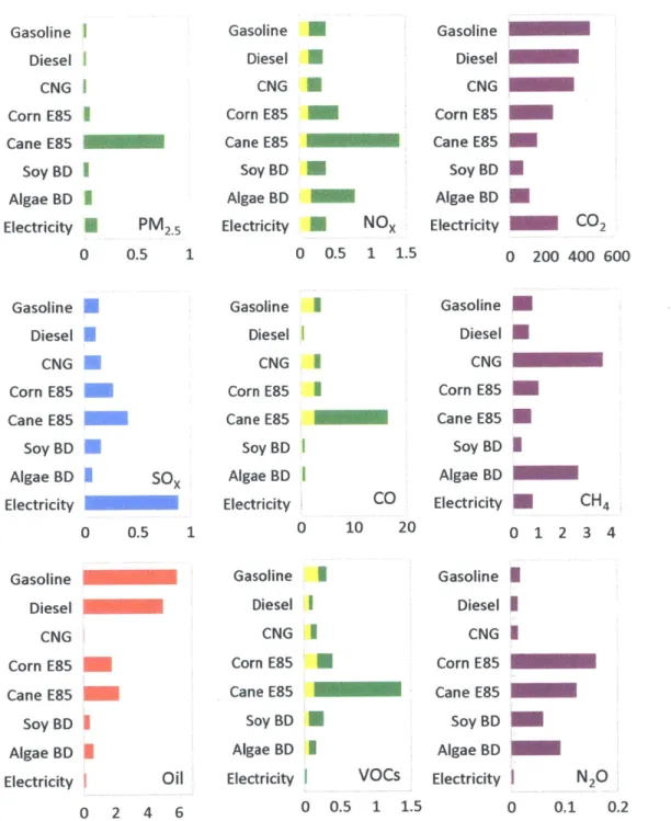
to comparing multiple categories (e.g. the "climate/water nexus"). See Fig. 2.2 for a subset of criteria over which fuels might be judged. Often when assessing environmental impacts, impacts within categories are weighted and aggregated into a single impact score; these scores are then weighted and aggregated again into an overall measure of environmental impact. Choosing a weighting scheme requires evaluations of uncertain scientific information, predictions about the evolution of human and natural systems, and judgements about the relative harm of different impacts, which may be nonlinear given the presence of thresholds in environmental systems. Since fuels vary in the types of environmental impacts they create, weighting schemes can have a dramatic influence on the perceived attractiveness of technologies options. We would also expect preferred weighting schemes to vary across locations, over time, and among different stakeholders [104].

Biofuels. The environmental impacts of biofuels, and particularly their climate impacts, are highly contentious. Although biofuels can theoretically have net zero greenhouse gas

Gasoline Diesel CNG Corn E85 Cane E85 Soy BD Algae BD Electricity Gasoline Diesel CNG Corn E85 Cane E85 Soy BD Algae BD Electricity Gasoline Diesel CNG Corn E85 Cane E85 Soy BD Algae BD Electricity I PM _2.5 0 0.5 Gasoline Diesel CNG Corn E85 Cane E85 Soy BD Algae BD Electricity 0 1 Gasoline Diesel CNG Corn E85 Cane E85 Soy BD U Algae BD Oil Electricity 0 2 4 6 NOx 0 0.5 1 1.5 Gasoline Diesel CNG Corn E85 Cane E85 Soy BD Algae BD Electricity I Gasoline Diesel I CNG I Corn E85

-A

U

Figure 2.2: Transportation fuels are difficult to compare because they carry a variety of

environmental impacts. Purple denotes climate impacts, yellow urban air pol-lution, green general air polpol-lution, blue acid rain, and red energy security. Emissions are given in grams per mile and petroleum (oil) consumption in

BTU per mile. Data source: GREET Version 2012.

emissions, since the CO2 released during fuel combustion is removed from the atmosphere

by biofuel crops as they grow, a full life cycle assessment reveals that these fuels can be

quite greenhouse gas intensive and carry a wide variety of other environmental impacts.

1 Gasoline Diesel CNG Corn E85 Cane E85 Soy BD Algae BD Electricity

First generation biofuels, which currently dominate biofuel markets, often rely on energy, fertilizer, and irrigation-intensive farming practices, which lead to greenhouse gas emissions and other negative environmental impacts [39, 46, 47, 66, 119]. Emissions from land use changes are also a critical concern [76, 111]. Converting land from other natural states, for example forests and wetlands, releases greenhouse gases, and it can take years for a biofuel to overcome this carbon deficit and begin to generate a net climate benefit [21]. Determining land use change emissions requires an assessment of how biofuel production will impact agricultural markets more broadly, and how much and what type of land will be converted to meet increased demand. Given the uncertain environmental impacts of first generation biofuels, there have been active debates as to whether these fuels have net energy and climate benefits over conventional fuels [29].

Part of the impetus for investing in second and third generation biofuels is to alleviate the environmental impacts inherent in first generation biofuels. Second generation biofuels show promise from an environmental perspective, since they are often a byproduct of other agricultural processes or grown on less favorable land. However, these fuels still impact the environment [7, 106, 119]. Agricultural waste already has uses in the agricultural system (for example, as a fertilizer) and must be replaced if waste products are used as a biofuel; other second generation crops still require land use changes and incur emissions from these changes [21, 76]. Nevertheless, second generation biofuels tend to improve on first generation options in terms of environmental impacts. Third generation biofuels, which have been engineered especially for biofuel production, could also have lower environmental impacts and greenhouse gas emissions. However, controlling the growing environment to optimize third generation biofuel production, for example through CO2 feeding, can be

resource-intensive and environmentally damaging [13, 15]. Other environmental issues with third generation biofuels are very fuel-specific; for example, CH4 leakage is a critical concern for

algae biofuel production [33].

Natural Gas. Natural gas essentially is CH4, and it burns to produce CO2. However,

when considering the life cycle greenhouse gas emissions of natural gas, the fugitive CH4 emissions that occur during gas production and transportation are critical. The rise in unconventional gas has also led scientists and policymakers to question how its CH4 emissions

compare to those of conventional gas [116]. Some have even argued that, depending on CH4 leakage rates during well completion, the CO2-equivalent greenhouse gas emissions of

natural gas may be worse than those of coal, which is far more C02-intensive [44]. Other

authors have criticized these findings [11], but an active debate continues in the policy community. The comparison of conventional and unconventional gas is complicated because conventional sources have additional CH4 emissions from liquid unloading, which is typically

not performed for unconventional sources [106, 118]. Given the high climate impacts of CH4, it is clear that more data on current practices is needed [5, 45]. Beyond its climate

impact, unconventional natural gas is also mined in locations not accustomed to oil and gas production. Among other community impacts, there is particular concern about gas contamination of water resources [73]. However, natural gas has fewer local and regional air quality impacts than many other fuel options.

Electricity. Electric vehicles have no direct emissions during vehicle driving since there

is no fuel being directly combusted in the vehicle. However, there are significant upstream emissions associated with the extraction, generation, and transmission of the electricity used to power electric vehicles, and these emissions must be counted in a full life cycle assessment. These emissions depend on the electricity generation mix, and can vary depending on the time of day and the geographical location of vehicle charging. The current electricity mix in the

U.S. is fairly fossil fuel and carbon-intensive, although studies suggest that electric vehicles in

the U.S. still do have climate benefits over conventional gasoline vehicles [27]. While electric vehicles eliminate some of the local air pollution concerns associated with conventional and alternative fuels, they tend to perform worse in terms of regional air quality, particularly acid rain, due to emissions from coal-fired power plants (see Fig. 2.2). However, it may be easier to mitigate climate and environmental impacts in the electricity sector, both because the emissions sources are easier to control and because there are more options for decarbonizing the electricity mix. Therefore, the impacts of electric vehicles may decrease significantly in the future.

2.2

Climate Metrics and Policy

2.2.1

Greenhouse Gases and Climate

The Earth's climate is a highly complex system driven by dynamic interactions between the atmosphere, lithosphere, hydrosphere, and biosphere. Historically, the Earth has experienced periods of rapid climate change due to internal feedbacks among these subsystems, which are often characterized by nonlinear or threshold behavior, and external influences on the climate, called forcings [4]. While these forcings can take many forms, recent climate changes are attributed to human-induced changes in the Earth's energy, or radiative, balance [102]. This phenomenon is referred to as radiative forcing.' Radiative forcing operates through two processes. First, when energy reaches the Earth's surface, part of this energy is re-radiated

5 _{Radiative forcing is measured in units of energy imbalance per unit time (or power imbalance) per unit}

back into the atmosphere. While some of this energy radiates back out into space, a portion of it is also absorbed by certain gases and reradiated back towards the Earth's surface. This blanketing effect, which is responsible for keeping the Earth's temperature hospitable to humans and other forms of life, is called the greenhouse effect, and the gases that produce this effect are called greenhouse gases. Second, some forcings, such as aerosols and black carbon, can effect the Earth's energy balance by absorbing or reflecting sunlight directly.

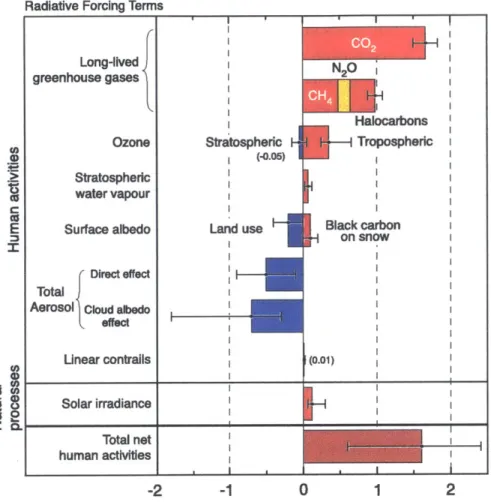
The most conmon greenhouse gases, in terms of their total greenhouse effect, are water vapor and CO2. CO2 represents the largest human contribution to climate change. However,

a host of secondary greenhouse gases and climate forcings, many of which are largely emitted

by humans, are also influential (see Fig. 2.3). Together, these secondary gases contribute

almost as much radiative forcing as CO2. In fact, while policy discussions often simplify the

climate problem to a "carbon" (i.e. C0 2) problem, it may be impossible to meet

commonly-cited climate goals without addressing non-CO2 radiative forcing [85]. After C0 2, which

represents 63% of long-lived forcings, CH4 is the second largest contributor to persistent

forcing, at 18%, followed by N20 at 6%, with the contribution of the latter growing rapidly

in recent years [102]. While ozone depleting compounds influenced the initial development of climate metrics, these substances represent a small share of total forcing, at around 12% combined, and their radiative forcing has declined in absolute terms since the late 1990's [102].

Linking radiative forcing perturbations to actual climate impacts is challenging. Increases in radiative forcing are expected to lead to a number of impacts, which the United Nations Framework Convention on Climate Change (UNFCCC) collectively terms "dangerous an-thropogenic interference" (DAI) [112] and later refined to include five "reasons for concern" (RFCs) [69]. In science policy discussions, DAI is most frequently operationalized as a 2*C temperature threshold, which was formalized by the UNFCCC in 2009 [114]. In addition to its political importance, the 2*C threshold also has scientific significance, and is a commonly-cited safe level for avoiding large-scale discontinuities in the climate system,6 _{one of the most}

critical RFCs [101]. However, the climate impacts resulting from an increasing abundance of greenhouse gases are complex and highly uncertain, and are likely to be unevenly dis-tributed across locations and disproportionately borne by future generations. Furthermore, given the potential for non-linear and irreversible changes to the climate, balancing the costs and benefits of greenhouse gas emissions is a difficult proposition.

Connecting greenhouse gases and climate impacts is further complicated by the fact that these gases have very different physical properties. Compared to C0 2, CH4 and N20 are

much more efficient at trapping heat: a gram of CH4 traps 102 times as much energy as a 60ther safe levels of climate change has also been proposed (see [63]). Note that many consider the 2 C thresholds to be too high for vulnerable regions and populations.

Radiative Forcing Terms Long-lived greenhouse gases Ozone Stratospheric water vapour Surface albedo, Direct effect Total

Aerosol Cloud abedo

Linear contrails Solar irradiance Total n t human activities -2 Stratospheric --0.05) Land use -1 0 1

Figure 2.3: Since pre-industrial times, there have been human-induced and natural changes

to the Earth's radiative forcing budget (in W/m2). The total effect of human activities is positive (i.e. warming), although the exact value is subject to con-siderable uncertainty, which is largely driven by uncertainties in aerosol physics and chemistry. Image source: [102].

gram of C0 2; a gram of N20 traps 216 times as much (see Fig. 2.4). These three gases also

have different lifetimes in the atmosphere, with CH4 being removed in a matter of decades

and N20 on the order of a century. The removal of CO2 is governed by a complex process

of continual exchange with carbon sinks in the ocean and biosphere; some CO2 is removed

almost instantaneously, while some CO2 is essentially permanent on timescales meaningful

for climate policy (i.e. thousands of years), and the average lifetime is on the order of a hundred years [103]. Other climate forcings such as aerosols, black carbon, and ozone have much shorter lifetimes (i.e. less than a year), and many ozone depleting substances have much longer lifetimes (i.e. thousands of years). Given their diverse physics, there is no single exchange rate that objectively converts one greenhouse gas into an equivalent amount of another gas. The exchange rate inevitably involves value judgements.

S 0 C 0 E I 0 z I. 2 0 N20 Halocarbons Tropospheric I Black carbon I on snow I (0.01) I

3 A. B. 52 150 300 X CH_{4 ; f} -100 50 75 1001 C0 -200 4N-0 CM 50 M 100 - N₂0 E _E 0 0 0 0 20 40 60 80 100 0 20 40 60 80 100

Time Since Emission (years) Time Since Emission (years)

Figure 2.4: (A.) CH4 and (B.) N20 have a higher radiative forcing per grain than C0 2;

however, their emissions decay at different rates in the atmosphere. As a result, the radiative forcing of a gram of C0 2, CH4, and N20 changes over time, with

CO2 and CH4 having equal radiative forcing 67 years after the emissions occur

and the radiative forcing contribution from of N20 remaining larger than CO2

through the 100-year period examined. Data source: [102].

2.2.2 History of Climate Metrics

Contemporary climate metrics were not initially designed for climate policy. They were de-veloped in the context of the Montreal Protocol, which regulates ozone depleting substances

[79]. Since some ozone depleting substances are also greenhouse gases, there was interest

in how ozone policies might have secondary effects on climate change. In 1988, Rogers and Stephens proposed the first measure for comparing the climate impacts of ozone depleting substances, which they called the greenhouse warming potential [94]. This metric was in-spired by the ozone depleting potential (ODP), a metric proposed by Wuebbles in 1983 to compare the steady state ozone depletion resulting from a step change in the emission of a substance, compared to the reference CFC- 11 [120].' In 1990, Fisher et al. proposed a similar metric, the halocarbon global warming potential (HGWP), which in parallel with the ODP compared the steady state radiative forcing of ozone depleting compounds [31]. The HGWP was also incorporated in reports by the United Nations Environment Program (UNEP) on stratospheric ozone, indicating that the idea of climate metrics was gaining traction in the policy community [1].

The HGWP concept, legitimized under the Montreal Protocol and initially restricted to ozone depleting compounds, was later extended to other greenhouse gases by Lashof and

7_{The destruction of stratospheric ozone by ozone depleting substances can be well approximated as a} linear function of concentration. As a result, the steady state impact of a step change in emissions is equivalent to the integrated impact of a pulse emission from the time of emission to the time steady state is reached (see [77]). The same reasoning applies to for the GWP concept when restricted to ozone depleting substances, since these substances exhibit an approximately linear relationship between concentration and radiative forcing, but does not apply for common greenhouse gases such as C02, CH4, and N20.

400 200

Ahuja [62]. The authors proposed the global warming potential (GWP) as the radiative forcing due to an emission of a greenhouse gas at t = 0, relative to an equivalent mass emission of C0 2, integrated to infinity, where future radiative forcing was discounted using

standard economic procedures:8'9

f"

GWP (GHG) =fo RF (C ) t dt (2.1)

f

where RF denotes the radiative forcing of a given greenhouse gas (GHG or C0 2), and r is

the discount rate. Rodhe proposed an alternative formulation, which integrates radiative forcing over a fixed time horizon:

f

GWP (GHG)=- 07' (2.2)

fj RF(CO2)dt '

where T is the time horizon [93]. This is equivalent to a special case of the Lashof and Ahuja formulation, where the discount function is equal to one up to time T and zero afterwards. Derwent subsequently extended Rodhe's work by calculating the GWP for three example time horizons: 20, 100, and 500 years [22].

The Intergovernmental Panel on Climate Change (IPCC), a scientific body established

by the United Nations to address climate change, later picked up the Rodhe formulation with

the three time horizons proposed by Derwent, introducing the modern GWP formulation to the policy community [43]. The IPCC emphasized the uncertainties in the GWP concept

and stated in particular that the three example time horizons were "presented as candidates for discussion and should not be considered as having any special significance" [42, page 59].

In spite of these reservations, the GWP with a 100 year time horizon was adopted by the Kyoto Protocol in 1998 as a basis for regulating greenhouse gas emissions [113]. Values for the GWP were taken from the then latest IPCC report [61] but have not been revised since, although the protocol explicitly states that the GWP should be periodically reviewed and revised:

"...the Conference of the Parties serving as the meeting of the Parties to the Protocol shall regularly review and, as appropriate, revise the global warming

8_{The analogy between step emissions and integrated pulse emissions does not hold for C0}

2, CH4, and

N20, which have a non-linear relationship between concentration and radiative forcing. This meant that

Lashof and Ahuja needed to make an explicit choice between the two formulations. They chose the latter to emphasize the impacts of individual emissions decisions, as opposed to emissions trends [77].

9_{Since some portion of CO}

2 emissions remain in the atmosphere essentially permanently, Lashof and

Ahuja forced the CO2 removal function to zero after a time period of 1,000 years to prevent the denominator

from reaching infinity. However, although the choice of time period was fairly arbitrary, they found that their GWP changed significantly depending on the time period selected.

potential of each such greenhouse gas, taking fully into account any relevant decisions by the Conference of the Parties." [113, p. 6].

Since its introduction, the GWP has triggered various critiques [68]. Suggestions for addressing these critiques range from relatively small changes, such as updating GWP values based on new scientific information and climate conditions [98, 102], to intermediate changes such as changing the time horizon for calculating the GWP [82], to dramatic changes, such as changing from the integrated, radiative forcing-based GWP to an instantaneous, temperature based global temperature potential (GTP) [100] (see [341 for a review). Some economists argue that metrics should explicitly balance the costs of climate change with benefits derived from activities that emit greenhouse gases, either by translating simple physical metrics into measures of economic damages or by simulating tradeoffs between gases in an integrated assessment model [67, 90]. However, reaching a consensus on the value of costs and benefits is extremely difficult, if not impossible [37]. Given the many inherent scientific, political, and economic uncertainties, some argue that the GWP is "good enough" for its intended application, at least under certain assumptions [36, 78].

To avoid these normative issues, some scientists favor grouping gases based on their physics, and prohibiting comparisons between groups [18]. This policy avoids the perverse tradeoffs inherent in greenhouse gas trading: since a fraction of CO2 emissions remain in

the atmosphere indefinitely, trading a temporary decrease in CH4 for a temporary increase

in CO2 hurts prospects for long-term climate stabilization [68]. At the same time, since the

climate system is complex and nonlinear, temporary increases in radiative forcing can lead to long-term, possibly permanent, impacts. Furthermore, studies find that allowing greenhouse gas trading reduces the total costs of climate change mitigation [90]. More fundamentally, climate metrics have important applications for which methods for grouping gases are in-appropriate. In technology assessments, technologies are routinely compared based on their C02-equivalent emissions. While complex models could theoretically simulate the impacts of

multi-gas emissions from technologies, this approach is too cumbersome for informing fine-grained technology choices, such as those required to select technology portfolios, prioritize among new designs in the laboratory, and set technology performance targets. For these applications, comparing gases on a single scale is difficult but necessary.

2.2.3

Questions for Designing Metrics

Given the strong argument for comparing greenhouse gases on a common scale, how can we do this better? Early debates on the benefits and drawbacks of popular climate metrics emphasized that metrics cannot be evaluated until a set of evaluation criteria is identified

produce identical radiative forcing pathways across all possible combinations of greenhouse gas emissions. I suggest that the major science policy debates that emerge out of the design and evaluation of climate metrics can be analyzed in the context of four major questions: (1) at what step in the emissions-to-impacts chain should we compare gases?, (2) should we use an instantaneous, integrated, or rate-based indicator?, (3) how should we balance short-term and long-term climate changes?, and (4) should climate metrics change over time or adapt to new information? I discuss each of these important questions below.

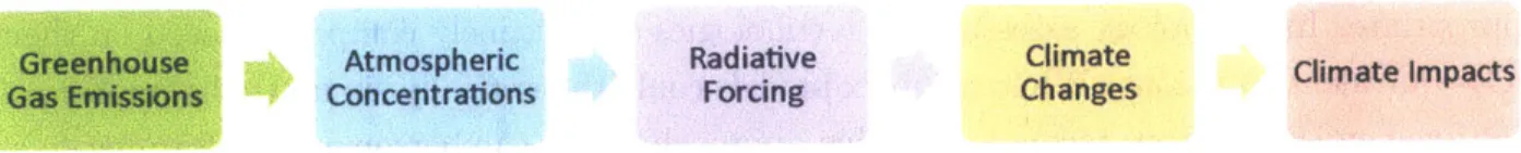
At what step in the emissions-to-impacts chain should we compare gases? Cli-mate science, economics, and policy research seeks to understand the complex process that relates emissions of greenhouse gases to damages to human wellbeing and the natural envi-ronment. Several steps along this chain could be selected as a basis for comparing greenhouse gases, ranging from radiative forcing to climate impacts (see Fig. 2.5). Steps at the begin-ning and the end of the chain have inherent tradeoffs. Steps near the beginbegin-ning are easier to measure, whereas steps near the end are more uncertain and difficult to quantify; however, steps near the end are also more meaningful for policymaking. This tradeoff relates to a broader literature on performance indicators. One analysis organizes indicators into three groups: (1) behavioral indicators, which measure the performance of individual actors, (2) intervening indicators, which measure performance somewhere along a causal chain, and

(3) consummatory indicators, which measure performance in terms of ultimate policy goals [91]. Radiative forcing and temperature change (intervening indicators) are common

indi-cators for comparing greenhouse gases, although rudimentary estimates of climate damages (consummatory indicators) are also sometimes used. Greenhouse gas emissions indicators (behavioral indicators) are more common in other areas of climate policy.

Greenhouse Atmospheric Radiative Climate Climate Impacts GasEmissions Concentrations Forcing Changes

Figure 2.5: Simple causal chain tracing greenhouse gas emissions to ultimate climate im-pacts. Moving down the causal chain, metrics become more uncertain and difficult to quantify but also more policy-relevant. Adapted from: [34].

Should we use an instantaneous, integrated, or rate-based indicator? After

se-lecting the indicator for comparing greenhouse gases, we must determine how this indicator will be formatted. Options include rates of change in the indicator, the total magnitude of the indicator, the indicator value integrated over time, or a hybrid of these three approaches.

radiative forcing can determine the ability of human and natural systems to adapt to climate changes, with slower rates allowing more time to adapt. At the same time, the magnitude of radiative forcing can govern ultimate changes to the climate system, such as temperature changes or increases in extreme weather events. On the other hand, climate damages are commonly associated with cumulative radiative forcing, with the important exception of non-linear and threshold effects. These three values may also be correlated. For instance, higher rates of change in radiative forcing lead to a higher magnitude of forcing and higher cumulative forcing. For this reason, maximum temperature change (an instantaneous mea-sure) is often cited as a broad policy target that roughly correlates with other secondary indicators of interest, including climate damages. However, others argue that climate policy must move beyond this simplistic approach to a more nuanced understanding of climate change indicators and safety thresholds [63].

How should we balance short-term and long-term climate impacts? Regardless of the indicator selected for comparing greenhouse gases, the treatment of time is critical.

Greenhouse gases vary widely in terms of their potencies and atmospheric lifetimes (see Fig. 2.4). Given these dramatically different properties, the emphasis placed on short-term versus long-term impacts can greatly affect the comparison of greenhouse gases, particularly

CO2 and CH4 and to a lesser extend CO2 and N20. If we compare one gram of CH4 to one

gram of CO2 at the time these gases are emitted, the impact of CH4 is over one hundred

times higher than that of CO2. If instead we compare these gases seventy years after they are

emitted, the impacts are almost equal. Thus, technologies with high CH4 emissions perform

worse in short-term impact assessments, whereas those with high CO2 emissions perform

worse in long-term assessments. These difficulties in balancing short-term and long-term impacts relate to a broader literature in environmental economics (and other economics disciplines) on discounting future costs and benefits [37]. Definitions of intergenerational equity and fairness in these complex systems are not objective and may vary across different stakeholders, some of whom do not have a voice in the policy process.

Should climate metrics change over time or adapt to new information? Beyond

issues concerning the appropriate indicator and treatment of time, many other types of spe-cialized science, technology, and policy knowledge are required to design and calculate cli-mate metrics. Scientific information about greenhouse gases - including their heat-trapping abilities, atmospheric lifetimes, and effects on other greenhouse gases - is constantly evolv-ing (see [98]). Many of these variables are also expected to change over time; for example, greenhouse gases tend to trap heat less efficiently as their concentrations increase. As a result, the tradeoffs between greenhouse gases change as relative concentrations increase or