HAL Id: hal-01122575
https://hal.archives-ouvertes.fr/hal-01122575
Submitted on 4 Mar 2015
HAL is a multi-disciplinary open access
archive for the deposit and dissemination of
sci-entific research documents, whether they are
pub-lished or not. The documents may come from
teaching and research institutions in France or
abroad, or from public or private research centers.
L’archive ouverte pluridisciplinaire HAL, est
destinée au dépôt et à la diffusion de documents
scientifiques de niveau recherche, publiés ou non,
émanant des établissements d’enseignement et de
recherche français ou étrangers, des laboratoires
publics ou privés.
Masses of negative multinomial distributions:
Application to Polarimetric Image Processing
Philippe Bernardoff, Florent Chatelain, Jean-Yves Tourneret
To cite this version:
Philippe Bernardoff, Florent Chatelain, Jean-Yves Tourneret. Masses of negative multinomial
distri-butions: Application to Polarimetric Image Processing. Journal of Probability and Statistics, Hindawi
Publishing Corporation, 2013, vol. 2013, pp. 1-13. �10.1155/2013/170967�. �hal-01122575�
O
pen
A
rchive
T
OULOUSE
A
rchive
O
uverte (
OATAO
)
OATAO is an open access repository that collects the work of Toulouse researchers and
makes it freely available over the web where possible.
This is an author-deposited version published in :
http://oatao.univ-toulouse.fr/
Eprints ID : 12404
To link to this article : DOI :10.1155/2013/170967
URL :
http://dx.doi.org/10.1155/2013/170967
To cite this version : Bernardoff, Philippe and Chatelain, Florent and
Tourneret, Jean-Yves
Masses of negative multinomial distributions:
Application to Polarimetric Image Processing
. (2013) Journal of
Probability and Statistics, vol. 2013. pp. 1-13. ISSN 1687-952X
Any correspondance concerning this service should be sent to the repository
administrator:
[email protected]
Research Article
Masses of Negative Multinomial Distributions:
Application to Polarimetric Image Processing
Philippe Bernardoff,
1Florent Chatelain,
2and Jean-Yves Tourneret
31Universit´e de Pau et des Pays de l’Adour, Avenue de l’Universit´e, 64012 Pau, France
2Gipsa-Lab, D´epartement Images et Signal, 961 rue de la Houille Blanche, BP 46, 38402 Saint Martin d’H´eres, France 3Universit´e de Toulouse, IRIT/ENSEEIHT/TESA, 2 rue Charles Camichel, BP 7122, 31071 Toulouse Cedex 7, France
Correspondence should be addressed to Florent Chatelain; [email protected]
This paper derives new closed-form expressions for the masses of negative multinomial distributions. These masses can be maximized to determine the maximum likelihood estimator of its unknown parameters. An application to polarimetric image processing is investigated. We study the maximum likelihood estimators of the polarization degree of polarimetric images using different combinations of images.
1. Introduction
The univariate negative binomial distribution is uniquely defined in many statistical textbooks. However, extensions defining multivariate negative multinomial distributions (NMDs) are more controversial. Most definitions are based on the probability generating function (PGF) of these distri-butions. Doss [1] proposed to define the PGF of an NMD as the inverse𝜆th power of a polynomial linear in each of its variables. This definition can also be found in the famous textbook [2, page 93] and the computation of its modes has been investigated in [3]. A more general class of NMDs introduced in [4] was characterized by PGFs of the form |I − Q|𝜆|I − QZ|−𝜆, where 𝜆 > 0, Q is an 𝑛 × 𝑛 matrix,
and Z = diag(𝑧1, . . . , 𝑧𝑛). In particular, matrices Q yielding infinitely divisible PGFs were derived. Finally, Bar-Lev et al. [5] introduced NMDs whose PGFs are defined as the inverse 𝜆th power of any affine polynomial. Necessary and sufficient conditions on the coefficients of this affine polynomial were derived to obtain the PGF of a multivariate distribution defined on N𝑛0(where N0is the set of nonnegative integers)
[6]. These very general multivariate NMDs were recently used for image processing applications in [7].
The family of NMDs introduced in [5] can be defined as follows. Let us denote [𝑛] = {1, . . . , 𝑛} the set of the 𝑛 first nonzero integers. We denote z𝑇 = ∏
𝑡∈𝑇𝑧𝑡 as the
monomial obtained by multiplying all the entries of the vector
z = (𝑧1, . . . , 𝑧𝑛) ∈ R𝑛 whose indexes belong to 𝑇, where 𝑇 ⊂ [𝑛] stands for any subset of the indexes. Let 𝑃𝑛(z) =
∑𝑇⊂[𝑛],𝑇 /== 0𝑝𝑇z𝑇be an affine polynomial with respect to the
𝑛 variables (𝑧1, . . . , 𝑧𝑛) such that 1 − 𝑃𝑛(1) /== 0. The NMD
distribution defined at pair(𝑛, 𝑃𝑛) is represented by its PFG which is given by
GNM(𝑛,𝑃
𝑛)(z) = (1 − 𝑃𝑛(z)) −𝜆(1 − 𝑃
𝑛(1))𝜆. (1)
Such laws are denoted as NM(𝑛, 𝑃𝑛). However, as explained in [6], all couples (𝑛, 𝑃𝑛) do not provide a valid NMD. More specifically, Bernardoff has derived a finite number of conditions over𝑃𝑛such that(1 − 𝑃𝑛(z))−𝜆(1 − 𝑃𝑛(1))𝜆is the PGF of an NMD for all positive integer𝑛. The corresponding expression of the coefficient of z𝛼in the Taylor expansion of (1 − 𝑃𝑛(z))−𝜆is given by the formula
𝑐𝛼(𝜆, 𝑃𝑛) = ∑
𝑘∈𝐾𝛼
(𝜆)|𝑘|p 𝑘
where𝐾𝛼= {𝑘 : P𝑛 → N} and P𝑛is the set of all subsets of [𝑛]. However, this expression of 𝑐𝛼(𝜆, 𝑃𝑛) does not allow us to
explicitly compute the masses of NMDs in the general case. As a first goal of this paper, we propose a way of com-puting the masses of multivariate NMDs NM(𝑛, 𝑃𝑛) defined above. A specific attention is devoted to bivariate and trivari-ate cases. In particular, it allows us to retrieve the results of [7] obtained for bivariate NMDs. The second part of the paper is devoted to the application of NMDs to image processing, more specifically to polarimetric image processing [8, 9]. Polarimetric image processing has received a considerable attention in the image processing and optical communities (see for instance [10–12] and references therein). The state of polarization of a polarimetric image is classically character-ized by the degree of polarization (DoP) whose estimation is of major importance [13, 14]. The DoP of polarimetric images can be classically estimated by using four images associated to four different polarizations [15]. However, estimating the DoP using less than four images is interesting since it allows one to reduce the acquisition time and the resulting cost of the imaging system. As a consequence, there has been recently an increasing interest in deriving estimators of the DoP based on a reduced number of polarimetric images. Depending on the intensity of the acquired images, polari-metric images are referred to as low flux or high flux images (low flux corresponding to a small intensity and high flux to a larger intensity). DoP estimation based on a single polari-metric image was considered in [16, 17] under high flux and low flux assumptions. DoP estimators derived from two intensity images degraded by fully developed speckle noise were studied in [18, 19]. Finally, imaging systems using three polarimetric images were studied in [20, 21], under high flux and low flux assumptions.
This paper studies the maximum likelihood estimators (MLEs) of the square DoP based on two or three polarimetric images. These estimators are computed by maximizing the masses of bivariate or trivariate NMDs derived in the first part of this work.
The paper is organized as follows. Section 2 recalls impor-tant results on NMDs. Section 3 proposes a new way of com-puting masses of NMDs. A particular attention is devoted to bivariate and trivariate cases. Section 4 addresses the problem of estimating the square DoP of low flux polarimet-ric images using the maximum likelihood (ML) principle. Different MLEs are constructed depending on the number of available polarimetric images. Simulation results are pre-sented in Section 5.
2. Negative Multinomial Distributions
An𝑛-variate NMD is the distribution of a random vector N = (𝑁1, . . . , 𝑁𝑛) taking its values in N𝑛0whose PGF is
𝐺N(z) = E ( 𝑛 ∏ 𝑘=1𝑧 𝑁𝑘 𝑘 ) = [𝑃𝑛(z)]−𝜆, (3)
where E denotes the mathematical expectation, z= (𝑧1, . . . , 𝑧𝑛), 𝜆 > 0, and 𝑃𝑛(z) is an affine polynomial of order 𝑛. (A polynomial𝑃𝑛(z) with respect to z = (𝑧1, . . . , 𝑧𝑛) is affine
if the one variable polynomial𝑧𝑗 ∣→ 𝑃𝑛(z) can be written as𝐴(−𝑗)𝑧𝑗 + 𝐵(−𝑗) (for any𝑗 = 1, . . . , 𝑑), where 𝐴(−𝑗) and 𝐵(−𝑗) are polynomials with respect to the𝑧
𝑖’s with𝑖 /== 𝑗.)
These discrete distributions have received much interest in the literature (see for instance [2] and the references therein). Of course, the affine polynomial𝑃𝑛has to satisfy appropriate conditions to ensure that𝐺N(z) is a PGF. These conditions include the trivial equality 𝑃𝑛(1, . . . , 1) = 1. However, determining all pairs (𝑃𝑛, 𝜆) such that 𝐺N(z) is a PGF is still an open problem (see [6], for discussions related to this problem). As explained in [6], the affine polynomial𝑃𝑛(z) can be rewritten
𝑃𝑛(z) = 𝐴𝑛𝐴(𝑎1𝑧1, . . . , 𝑎𝑛𝑧𝑛)
𝑛(𝑎1, . . . , 𝑎𝑛) , (4)
where 𝑎1, . . . , 𝑎𝑛 are positive numbers and𝐴𝑛 is an affine polynomial such that𝐴𝑛(0, . . . , 0) = 1. The Taylor expansions of[𝐴𝑛(z)]−𝜆and[𝑃𝑛(z)]−𝜆in the neighborhood of(0, . . . , 0) will be denoted as follows:
[𝐴𝑛(z)]−𝜆= ∑ 𝛼∈N𝑛 0 𝑐𝛼(𝜆, 𝐴𝑛) z𝛼, [𝑃𝑛(z)]−𝜆= ∑ 𝛼∈N𝑛 0 𝑐𝛼(𝜆, 𝑃𝑛) z𝛼, (5) where 𝛼 = (𝛼1, . . . , 𝛼𝑛) and z𝛼 = ∏𝑛𝑖=1𝑧𝑖𝛼𝑖. Equations (3) and (4) clearly show that the masses of multivariate NMDs denoted as𝑐𝛼(𝜆, 𝑃𝑛) can be expressed as follows:
𝑐𝛼(𝜆, 𝑃𝑛) = 𝑐𝛼(𝜆, 𝐴𝑛) ∏ 𝑛 𝑖=1𝑎𝛼𝑖𝑖 𝐴𝑛(𝑎1, . . . , 𝑎𝑛)−𝜆 . (6)
3. Masses of Negative
Multinomial Distributions
In this section, we derive new expressions for the coefficients 𝑐𝛼(𝜆, 𝐴𝑛) that will be used to compute the masses of NMDs.
The particular cases of bivariate and trivariate NMDs will play an important role for the estimation of the DoP on polarimetric images. In order to compute the𝑐𝛼(𝜆, 𝐴𝑛), we derive several results summarized in this section whereas all demonstrations are reported in the appendix.
Theorem 1. Denote P∗𝑛as the set of nonempty subsets of[𝑛] = {1, . . . , 𝑛}. Any affine polynomial 𝐴𝑛 such that 𝐴𝑛(0) = 1
denoted as
𝐴𝑛(z) = 1 − ∑
𝑇∈P∗
𝑛
𝑎𝑇z𝑇 (7)
can be expressed as follows: 𝐴𝑛(z) = ∏ 𝑖∈[𝑛](1 − 𝑎𝑖𝑧𝑖) −𝑇∈P∑∗ 𝑛,|𝑇|⩾2 𝑑𝑛 𝑇z𝑇 ∏ 𝑖∈[𝑛]\𝑇(1 − 𝑎𝑖𝑧𝑖) , (8)
where|𝑇| is the cardinal of the set 𝑇. Moreover 𝐴𝑛(z) = [∏ 𝑖∈[𝑛](1 − 𝑎𝑖𝑧𝑖)] × (1 − ∑ 𝑇∈P∗𝑛,|𝑇|⩾2𝑑 𝑛 𝑇 z 𝑇 ∏𝑖∈𝑇(1 − 𝑎𝑖𝑧𝑖)) (9) = [∏ 𝑖∈[𝑛](1 − 𝑎𝑖𝑧𝑖)] × (1 − 𝑄𝑛( 𝑧1 − 𝑎1 1𝑧1, . . . , 𝑧𝑛 1 − 𝑎𝑛𝑧𝑛)) , (10)
where 𝑄𝑛 is the polynomial defined by 𝑄𝑛(z) = ∑𝑇∈P∗
𝑛,|𝑇|⩾2𝑑
𝑛
𝑇z𝑇 and 𝑑𝑛𝑇 is related to the 2|𝑇| − 1 variables
𝑎𝑆, 𝑆 ∈ P∗𝑇as follows: 𝑑𝑛 𝑇= |𝑇| ∑ 𝑇∈P𝑛 |𝑇|>1 𝑎𝑇𝑎[𝑛]\𝑇+ (|𝑇| − 1) ∏ 𝑖∈𝑇𝑎𝑖. (11)
Remark 2. In the trivariate case defined by𝑛 = 3, the poly-nomial𝐴3(z) can be expressed as
𝐴3(z) = (1 − 𝑎1𝑧1) (1 − 𝑎2𝑧2) (1 − 𝑎3𝑧3) × [1 − 𝑄3( 𝑧1 1 − 𝑧1, 𝑧 2 1 − 𝑧2, 𝑧 3 1 − 𝑧3)] , (12)
where the coefficients of the polynomial
𝑄3(z) = 𝑏1,2𝑧1𝑧2+ 𝑏1,3𝑧1𝑧3+ 𝑏2,3𝑧2𝑧3+ 𝑏1,2,3𝑧1𝑧2𝑧3 (13)
can be determined using the relations
𝑏𝑖,𝑗= 𝑎𝑖,𝑗+ 𝑎𝑖𝑎𝑗, 𝑖, 𝑗 ∈ {1, 2, 3} , 𝑖 /== 𝑗,
𝑏1,2,3= 𝑎1,2,3+ 𝑎1𝑎2,3+ 𝑎2𝑎1,3+ 𝑎3𝑎1,2+ 2𝑎1𝑎2𝑎3.
(14)
The next theorem provides a relation between the coefficients of the polynomials𝐴𝑛(z) and 𝑄𝑛(z) introduced above.
Theorem 3. Let𝐴𝑛(z) = 1 − ∑𝑇∈P∗𝑛𝑎𝑇𝑧𝑇, a = (𝑎1, . . . , 𝑎𝑛),
and𝑄𝑛 be the affine polynomial defined in (10) and (11). For any 𝛼 and 𝛾 in N𝑛, denote as𝑐𝛾(𝜆, 𝐴𝑛) the coefficient of z𝛾 in the Taylor expansion of[𝐴𝑛(z)]−𝜆and as𝑐𝛼(𝜆, 1 − 𝑄𝑛) the
coefficient of z𝛼 in the Taylor expansion [1 − 𝑄𝑛(z)]−𝜆. The following relation can be obtained:
𝑐𝛾(𝜆, 𝐴𝑛) = ∑ 𝛼+𝛽=𝛾𝑐𝛼(𝜆, 1 − 𝑄𝑛) (𝜆1 + 𝛼)𝛽 a𝛽 𝛽! (15) = ∑ 0⩽𝛽𝑖⩽𝛾𝑖, 𝑖=1,...,𝑛 𝑐𝛾−𝛽(𝜆, 1 − 𝑄𝑛) ×∏𝑛 𝑖=1(𝜆 + 𝛾𝑖− 𝛽𝑖)𝛽𝑖 𝑎𝛽𝑖 𝑖 𝛽𝑖! (16) = ∑ 0⩽𝛼𝑖⩽𝛾𝑖, 𝑖=1,...,𝑛 𝑐𝛼(𝜆, 1 − 𝑄𝑛) ×∏𝑛 𝑖=1(𝜆 + 𝛼𝑖)𝛽𝑖 𝑎𝛾𝑖−𝛼𝑖 𝑖 (𝛾𝑖− 𝛼𝑖)!. (17)
The masses of NMDs can be directly obtained from this theorem. The particular cases of bivariate and trivariate NMDs are considered in the following subsections since the corresponding masses will be useful in the application considered in the second part of this paper.
3.1. Bivariate NMDs
Theorem 4. Consider the affine polynomial of order 2 with variables z= (𝑧1, 𝑧2) defined by
𝐴2(z) = 1 − ∑
𝑇∈P∗
2
𝑎𝑇𝑧𝑇= 1 − 𝑎1𝑧1− 𝑎2𝑧2− 𝑎1,2𝑧1𝑧2. (18)
The coefficient of z𝛾in the Taylor expansion of[𝐴2(z)]−𝜆, can be computed as follows 𝑐𝛾(𝜆, 𝑃2) = (𝜆)max(𝛾1,𝛾2) min(𝛾1,𝛾2) ∑ ℓ=0 (𝜆 + ℓ)min(𝛾1,𝛾2)−ℓ (𝛾1− ℓ)! (𝛾2− ℓ)!ℓ! × 𝑎𝛾1−ℓ 1 𝑎2𝛾2−ℓ𝑏1,2ℓ . (19)
Remark 5. The result (A.11) was mentioned in [7] without the factorization leading to (19). If𝑎1 /== 0 and 𝑎2 /== 0, an equivalent formulation of (19) is 𝑐𝛾(𝜆, 𝑃2) = 𝑎 𝛾1 1𝑎2𝛾2 𝛾1!𝛾2! (𝜆)max(𝛾1,𝛾2) × min(𝛾1,𝛾2) ∑ ℓ=0 (𝜆 + ℓ) min(𝛾1,𝛾2)−ℓ × (𝛾1 ℓ ) (𝛾ℓ ) ℓ!(2 𝑎𝑏11,2𝑎2) ℓ . (20) 3.2. Trivariate NMDs
Theorem 6. Consider the affine polynomial with the three variables z= (𝑧1, 𝑧2, 𝑧3) defined by 𝐴3(z) = 1 − ∑ 𝑇∈P∗ 3 𝑎𝑇𝑧𝑇. (21)
The coefficient of z𝛾in the Taylor expansion of[𝐴3(z)]−𝜆are 𝑐𝛾(𝜆, 𝑃3) = 𝛾1 ∑ 𝛽1=0 𝛾2 ∑ 𝛽2=0 𝛾3 ∑ 𝛽3=0 ⌊|𝛾−𝛽|/2⌋ ∑ 𝑣=‖𝛾−𝛽‖ (𝜆)𝑣 ×𝑏2,3𝑣−𝛾1+𝛽1𝑏1,3𝑣−𝛾2+𝛽2𝑏1,2𝑣−𝛾3+𝛽3 ∏3𝑖=1(𝑣 − 𝛾𝑖+ 𝛽𝑖)! 𝑏1,2,3|𝛾−𝛽|−2𝑣 (𝛾 − 𝛽 − 2𝑣)! ×(𝜆 + 𝛾1− 𝛽1)𝛽1 𝛽1! (𝜆 + 𝛾2− 𝛽2)𝛽2 𝛽2! ×(𝜆 + 𝛾3− 𝛽3)𝛽3 𝛽3! 𝑎1𝛽1𝑎𝛽22𝑎3𝛽3. (22) When 𝑎𝑖 /== 0, 𝑏𝑖,𝑗 /== 0, 𝑖 /== 𝑗, 𝑖 = 1, 2, 3, 𝑗 = 1, 2, 3, and 𝑏1,2,3 /== 0, an equivalent expression is 𝑐𝛾(𝜆, 𝑃3) = 𝑎1𝛾1𝑎2𝛾2𝑎𝛾33 𝛾1 ∑ 𝛽1=0 𝛾2 ∑ 𝛽2=0 𝛾3 ∑ 𝛽3=0 ⌊|𝛾−𝛽|/2⌋ ∑ 𝑣=‖𝛾−𝛽‖ (𝜆)𝑣 × (𝑏2,3𝑏1,3𝑏1,2/𝑏1,2,32 ) 𝑣 (𝛾 − 𝛽 − 2𝑣)!∏3 𝑖=1(𝑣 − 𝛾𝑖+ 𝛽𝑖)! × [∏3 𝑖=1 (𝜆 + 𝛾𝑖− 𝛽𝑖)𝛽𝑖 𝛽𝑖! ] ( 𝑏1,2,3 𝑎1𝑏2,3) 𝛾1−𝛽1 × (𝑎𝑏1,2,3 2𝑏1,3) 𝛾2−𝛽2 (𝑎𝑏1,2,3 3𝑏1,2) 𝛾3−𝛽3 (23) = (𝜆)‖𝛾‖a 𝛾 𝛾! 𝛾1 ∑ 𝛼1=0 𝛾2 ∑ 𝛼2=0 𝛾3 ∑ 𝛼3=0 ⌊|𝛼|/2⌋ ∑ 𝑣=‖𝛼‖ (𝜆 + ‖𝛼‖)𝑣−‖𝛼‖ (|𝛼| − 2𝑣)!∏3𝑖=1(𝑣 − 𝛼𝑖)! ×(𝑏2,3𝑏𝑏21,3𝑏1,2 1,2,3 ) 𝑣 𝛼!(𝑎𝑏1,2,3 1𝑏2,3) 𝛼1 (𝑎𝑏1,2,3 2𝑏1,3) 𝛼2 (𝑎𝑏1,2,3 3𝑏1,2) 𝛼3 ×∏3 𝑖=1[(𝜆 + 𝛼𝑖)𝛾𝑖−𝛼𝑖(𝛾 𝑖 𝛼𝑖)] . (24)
4. Estimating the Polarization Degree of
Low Flux Polarimetric Images Using
Maximum Likelihood Methods
4.1. Low Flux Polarimetric Images. The state of the polariza-tion of the light can be described by the random behavior of a complex vector A= (𝐴𝑋, 𝐴𝑌), called the Jones vector, whose covariance matrix, called the polarization matrix, is
Γ = (E[𝐴𝑋𝐴∗𝑋] E [𝐴𝑋𝐴∗𝑌]
E[𝐴𝑌𝐴∗𝑋] E [𝐴𝑌𝐴∗𝑌]) ≜ (
𝑎1 𝑎3+ 𝑖𝑎4
𝑎3− 𝑖𝑎4 𝑎2 ) ,
(25)
where∗ denotes the complex conjugate. The covariance matrixΓ is a nonnegative Hermitian matrix whose diagonal terms are the intensity components in the𝑋 and 𝑌 directions. The cross terms ofΓ are the correlations between the Jones components. If we assume a fully developed speckle, the Jones vector A is distributed according to a complex Gaussian distribution whose probability density function (pdf) is [15]: 𝑝 (A) = 1𝜋2|Γ| exp(−A†Γ−1A) , (26) where|Γ| is the determinant of the matrix Γ and † denotes the conjugate transpose operator. As a consequence, the statistical properties of A are fully characterized by the covariance matrixΓ. The different components of Γ can be classically estimated by using four intensity images that are related to the components of the Jones vector as follows (see [20], for more details):
𝐼1= 𝐴𝑋2,
𝐼2= 𝐴𝑌2,
𝐼3= 12𝐴𝑋2+ 12𝐴𝑌2+ Re (𝐴𝑋𝐴∗𝑌) ,
𝐼4= 12𝐴𝑋2+ 12𝐴𝑌2+ Im (𝐴𝑋𝐴∗𝑌) .
(27)
The state of the polarization of the light is classically charac-terized by the square DoP defined by [15, pages 134–136]
𝑃2= 1 − 4 |Γ| [trace (Γ)]2 = 1 − 4 [𝑎1𝑎2− (𝑎2 3+ 𝑎42)] (𝑎1+ 𝑎2)2 , (28) where trace(Γ) is the trace of the matrix Γ. The light is totally depolarized for𝑃 = 0, totally polarized for 𝑃 = 1, and par-tially polarized when𝑃 ∈ ]0, 1[. As a consequence, estimating the square DoP of a polarimetric image is important in many practical applications. Different estimation methods of 𝑃2 using several combinations of intensity images were studied in [20]. Since only one realization of the random vector I= (𝐼1, . . . , 𝐼4)𝑇was available for a given pixel of a polarimetric
image, the image was supposed to be locally stationary and ergodic. These assumptions were used to derive square DoP estimators using several neighbor pixels belonging to a so-called estimation window.
This paper considers practical applications where the intensity level of the reflected light is very low (low flux assumption), which leads to an additional source of fluctu-ations on the detected signal. Under the low flux assumption, the quantum nature of the light leads to a Poisson-distributed noise which can become very important relatively to the mean value of the signal at a low photon level. As a conse-quence, the observed pixels of the low flux polarimetric image are discrete random variables contained in the vector N = (𝑁1, . . . , 𝑁4) such that the conditional distributions of the random variables𝑁𝑙| 𝐼𝑙, for𝑙 = 1, . . . , 4 are independent and distributed according to Poisson distributions with means𝐼𝑙,
for 𝑙 = 1, . . . , 4. The resulting joint distribution of N is a multivariate mixed Poisson distribution [22]:
𝑃 (N = k) = ∫ ⋅ ⋅ ⋅ (R+)4 ∫∏4 𝑙=1 𝐼𝑘𝑙 𝑙
𝑘𝑙!exp(−𝐼𝑙) 𝑓(I) 𝑑I, (29)
where k= (𝑘1, . . . , 𝑘4), 𝑘𝑖∈ N, and 𝑓(I) is the joint pdf of the intensity vector. This section studies estimators of the square DoP𝑃2defined in (28) based on several vectors N1, . . . , N𝑛 belonging to the estimation window. These estimators are constructed from estimates of the covariance matrix elements 𝑎𝑖, 𝑖 = 1, . . . , 4. As explained in the introduction, several studies have been recently devoted to the estimation of the square DoP using less than four polarimetric images. This paper goes into this direction by deriving estimators based on the observation of 2 or 3 polarimetric images.
The joint distribution of the intensity vector I is known to be a multivariate gamma distribution whose Laplace trans-form is [20]
𝐸 [exp (∑4
𝑘=1𝑧𝑘𝐼𝑘)] = 1𝑃4(z), (30)
where the affine polynomial𝑃4is
𝑃4(z) = 1 + z𝜇 + 𝑘𝑎[2𝑧1𝑧2+ 𝑧3𝑧4+ (𝑧1+ 𝑧2) (𝑧3+ 𝑧4)] (31) with z= (𝑧1, . . . , 𝑧4) and 𝑘𝑎= 12 (𝑎1𝑎2− 𝑎32− 𝑎24) , 𝜇 = (𝑎1, 𝑎2, 𝑎3+ 𝑎12 , 𝑎+ 𝑎2 4+ 𝑎1+ 𝑎2 )2 𝑇 . (32)
As a consequence, the distribution of N is an NMD whose PGF can be written as (the interested reader is invited to consult [22] for more details)
𝐺N(z) =
1
𝑃4(𝑧1− 1, 𝑧2− 1, 𝑧3− 1, 𝑧4− 1). (33)
The results of Section 2 allow us to compute the masses of
Nthat will be useful for studying the maximum likelihood estimator (MLE) of the square DoP.
4.2. MLE Using Three Polarimetric Images. The PGF of ̃N =
(𝑁1, 𝑁2, 𝑁3) can be computed from (33) by setting 𝑧4 = 1.
The following result can be obtained: 𝐺̃N(z) = 1𝑃 3(z) (34) with 𝑃3(z) = 𝑃3(0) + 𝑧1(𝜇1− 3𝑘𝑎) + 𝑧2(𝜇2− 3𝑘𝑎) + 𝑧3(𝜇3− 2𝑘𝑎) + 𝑘𝑎(2𝑧1𝑧2+ 𝑧1𝑧3+ 𝑧2𝑧3) , (35)
z= (𝑧1, 𝑧2, 𝑧3), and 𝑃3(0) = 1 − ∑3𝑖=1𝜇𝑖+ 4𝑘𝑎. The results of Section 3.2 can then be used to express the masses of ̃Nas a function of𝜃 = (𝑎1, 𝑎2, 𝑎3, 𝑎42)𝑇.
The ML estimator of 𝜃 based on several vectors ̃N𝑘 belonging to the estimation window (where𝑘 = 1, . . . , 𝐾 and𝐾 is the number of pixels of the observation window) is obtained by maximizing the log-likelihood
𝑙3(̃N1, . . . , ̃N𝐾| 𝜃) = 𝐾
∑
𝑘=1
log [𝑃 (̃N𝑘)] (36)
with respect to 𝜃 (note again that 𝑃(̃N𝑘) is the mass of a trivariate NMD that has been computed in Section 3.2). The practical determination of the ML estimator of𝜃 is achieved by using a Newton-Raphson procedure. The ML estimators of the vector𝜃, denoted as ̃𝜃 = (̃𝑎1, ̃𝑎2, ̃𝑎3, ̃𝑎24)𝑇, are then plugged into (28) to provide the ML estimator of the square DoP based on three polarimetric images:
̃𝑃2= 1 −4 [̃𝑎1̃𝑎2− (̃𝑎32+ ̃𝑎24)]
(̃𝑎1+ ̃𝑎2)2
. (37)
4.3. MLE Using Two Polarimetric Images. The PGF of N = (𝑁1, 𝑁2) can be computed from (34) by setting 𝑧3 = 1. The
following result can be obtained: 𝐺N(z) = 1
𝑃2(z) (38)
with
𝑃2(z) = 𝑃2(0) + 𝑧1(𝜇1− 2𝑘𝑎) + 𝑧2(𝜇2− 2𝑘𝑎) + 2𝑘𝑎𝑧1𝑧2,
(39)
z = (𝑧1, 𝑧2) and 𝑃2(0) = 1 − ∑2𝑖=1𝜇𝑖+ 2𝑘𝑎. The results of Section 3.1 can then be used to express the masses of N as a function of𝜃 = (𝑎1, 𝑎2, 𝑘𝑎)𝑇.
The MLE of𝜃 based on several vectors N𝑘 belonging to the estimation window is obtained by maximizing the log-likelihood 𝑙2(N1, . . . , N𝐾| 𝜃) = 𝐾 ∑ 𝑘=1 log[𝑃 (N𝑘)] (40)
with respect to𝜃 (note that 𝑃(N𝑘) is the mass of a bivariate NMD that has been computed in Section 3.1). The practical determination of the ML estimator of𝜃 is achieved by using a Newton-Raphson procedure. The ML estimators of the vector
𝜃 elements, denoted as 𝜃 = (𝑎1, 𝑎2, 𝑘𝑎)𝑇, are then plugged
into (28) to provide the MLE of the square DoP based on two polarimetric images:
𝑃2= 1 − 8𝑘𝑎
Table 1: Covariance matrix elements and square DoP values for the Jones vector. Γ0 Γ1 Γ2 Γ3 Γ4 Γ5 Γ6 Γ7 Γ8 Γ9 Γ10 𝑎1 2.00 1.71 2.40 1.82 2.00 2.67 2.40 2.24 2.74 2.00 2.00 𝑎2 2.00 2.29 1.60 2.18 2.00 1.33 1.60 1.76 1.26 2.00 2.00 𝑎3 0.00 0.40 0.48 0.91 0.89 0.96 1.07 1.05 1.46 0.60 1.41 𝑎4 0.00 0.40 0.64 0.58 0.89 0.80 1.05 1.28 0.73 1.80 1.41 𝑃2 0 0.1 0.2 0.3 0.4 0.5 0.6 0.7 0.8 0.9 1.0
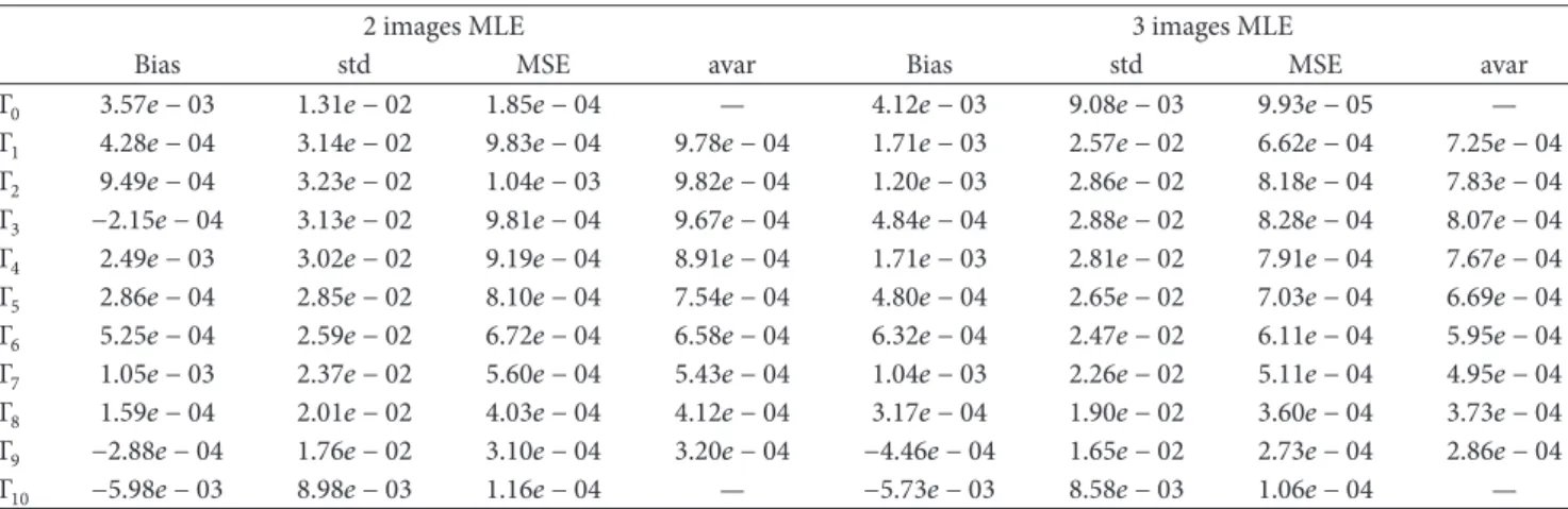
Table 2: Simulation results for the estimation of𝑃2using 2 or 3 images, obtained from1000 Monte-Carlo runs (𝑛 = 51 × 51).
2 images MLE 3 images MLE
Bias std MSE avar Bias std MSE avar
Γ0 3.57𝑒 − 03 1.31𝑒 − 02 1.85𝑒 − 04 — 4.12𝑒 − 03 9.08𝑒 − 03 9.93𝑒 − 05 — Γ1 4.28𝑒 − 04 3.14𝑒 − 02 9.83𝑒 − 04 9.78𝑒 − 04 1.71𝑒 − 03 2.57𝑒 − 02 6.62𝑒 − 04 7.25𝑒 − 04 Γ2 9.49𝑒 − 04 3.23𝑒 − 02 1.04𝑒 − 03 9.82𝑒 − 04 1.20𝑒 − 03 2.86𝑒 − 02 8.18𝑒 − 04 7.83𝑒 − 04 Γ3 −2.15𝑒 − 04 3.13𝑒 − 02 9.81𝑒 − 04 9.67𝑒 − 04 4.84𝑒 − 04 2.88𝑒 − 02 8.28𝑒 − 04 8.07𝑒 − 04 Γ4 2.49𝑒 − 03 3.02𝑒 − 02 9.19𝑒 − 04 8.91𝑒 − 04 1.71𝑒 − 03 2.81𝑒 − 02 7.91𝑒 − 04 7.67𝑒 − 04 Γ5 2.86𝑒 − 04 2.85𝑒 − 02 8.10𝑒 − 04 7.54𝑒 − 04 4.80𝑒 − 04 2.65𝑒 − 02 7.03𝑒 − 04 6.69𝑒 − 04 Γ6 5.25𝑒 − 04 2.59𝑒 − 02 6.72𝑒 − 04 6.58𝑒 − 04 6.32𝑒 − 04 2.47𝑒 − 02 6.11𝑒 − 04 5.95𝑒 − 04 Γ7 1.05𝑒 − 03 2.37𝑒 − 02 5.60𝑒 − 04 5.43𝑒 − 04 1.04𝑒 − 03 2.26𝑒 − 02 5.11𝑒 − 04 4.95𝑒 − 04 Γ8 1.59𝑒 − 04 2.01𝑒 − 02 4.03𝑒 − 04 4.12𝑒 − 04 3.17𝑒 − 04 1.90𝑒 − 02 3.60𝑒 − 04 3.73𝑒 − 04 Γ9 −2.88𝑒 − 04 1.76𝑒 − 02 3.10𝑒 − 04 3.20𝑒 − 04 −4.46𝑒 − 04 1.65𝑒 − 02 2.73𝑒 − 04 2.86𝑒 − 04 Γ10 −5.98𝑒 − 03 8.98𝑒 − 03 1.16𝑒 − 04 — −5.73𝑒 − 03 8.58𝑒 − 03 1.06𝑒 − 04 —
5. Simulation Results
5.1. Estimation Performance. The performance of the ML estimators of the square DoP based on two or three polari-metric images has been evaluated via several experiments. The first simulations compare the log Mean Square Errors (MSEs) of the square DoP estimators constructed from two or three images. Eleven different covariance matrices of the Jones vector have been considered in order to define typical values of the DoP. The values of𝑎𝑖, for𝑖 = 1, . . . , 4, (defining the covariance matrix elements of the Jones vector) and the corresponding values of the square DoPs are reported in Table 1. Note that all the covariance matricesΓ𝑗,𝑗 = 0, . . . , 10, have been normalized so that the mean of the total intensity
E[𝐼1+ 𝐼2] = E[𝑁1+ 𝑁2] = 𝑎1+ 𝑎2is equal to 4. Thus, the average number of photons collected on each pixel equals 4 for each matrix of the considered set. This point is in agreement with the low flux assumption.
Figure 1(a) display the empirical log MSEs of the square DoP estimators for the set of covariance matrices defined in Table 1 as a function of the true square DoP value. The red plus markers + correspond to the estimators obtained for two polarimetric images (2D MLE), whereas the blue cross markers× correspond to the MLE obtained for three polarimetric images (3D MLE). Note that these empirical MSEs have been computed for a square observation window of size𝑛 = 51 × 51 pixels, based on 1000 Monte-Carlo runs. The theoretical asymptotic log MSEs of the MLE are also dis-played in Figure 1(a) with continuous lines. These asymptotic values correspond to the Cramer-Rao Lower Bound (CRLB) for the parameter𝑃2. The MLE is known to be asymptotically unbiased and efficient under mild regularity conditions (that
are satisfied for𝑃2). Thus, the MSE of the estimates can be approximated a for large sample by the CRLB. More details about the way of computing the square DoP CLRBs can be found in [23]. Figure 1(a) indicates that the empirical MSEs are in good agreement with the corresponding CRLBs, except for the matrices Γ0 and Γ10. Indeed, the CRLBs for these two matrices cannot be computed since the true value of the parameters belongs to the boundary of its definition domain. The empirical bias, standard deviations (“std”), MSEs, and asymptotic variances (“avar”) of the estimators of𝑃2are also reported in Table 2. It is interesting to note that the MLE obtained using 3 images is slightly more biased than the one obtained using 2 images. However, the MLE based on 3 images provides lower MSEs than the estimator based on 2 images, as expected.
In order to appreciate the influence of the Poisson noise due to the low flux assumption, experiments have been conducted using the high flux assumption. In this case, the intensity vector I is assumed to be known. Thus, the high flux MLEs using two and three images can be derived from the intensity vectors I𝑘 = (𝐼1𝑘, 𝐼2𝑘)𝑇 and ̃I𝑘 = (𝐼1𝑘, 𝐼2𝑘, 𝐼3𝑘)𝑇[20]. The results are depicted in Figure 1(b). A comparison between Figures 1(a) and 1(b) allows one to appreciate a similar global behaviour for all the estimators, with a maximum MSE near 𝑃2 = 1/3 and decreasing MSEs as 𝑃2 goes to0 or 1. The
degradation of the estimation performance due to the pres-ence of Poisson noise (due to the low flux assumption) can also be clearly noticed.
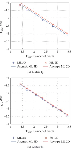
The next set of simulations studies the performance of the different estimators as a function of the sample size𝑛. Figures 2(a) and 2(b) show the log MSEs of the square DoP
log 10 MSE −2.6 −2.8 −3 −3.2 −3.4 −3.6 −3.8 −4 −4.2 0 0.2 0.4 0.6 0.8 1 P2 ML 2D Asympt. ML 2D ML 3D Asympt. ML 3D
(a) Low flux
log 10 MSE −3.2 −3.4 −3.6 −3.8 −4 −4.2 −4.4 −4.6 −4.8 −5 −5.2 0 0.2 0.4 0.6 0.8 1 P2 ML 2D Asympt. ML 2D ML 3D Asympt. ML 3D (b) High flux
Figure 1: log MSEs of the square DoP estimates using 2 and 3 images versus 𝑃2 for the set of polarization matrices defined in Table 1 under (a) low flux and (b) high flux assumptions (𝑛 = 51 × 51, ML: maximum likelihood estimators, and Asympt.: theoretical asymptotic value of the log MSE for a given estimator).
estimates obtained for2 and 3 images (for the two particular matricesΓ2andΓ8). The empirical bias, standard deviations (“std”), MSEs, and asymptotic variances (“avar”) are also reported in Tables 3 and 4. One can see that the empirical MSEs are in good agreement with their theoretical asymptotic values for a large enough sample size, that is,𝑛 > 25 × 25. Moreover, the gain of a performance using3 images instead of2 is more significant for small values of 𝑃2 (indeed, the difference between the different curves is more pronounced in the left figure corresponding to𝑃2 = 0.2 than in the right figure corresponding to𝑃2= 0.8.)
Figures 3(a) and 3(b) display the MSEs of the MLE under the high flux assumption. By comparing Figures 2 and 3, one can observe that the gain of performance using3 images instead of2 is more important in the high flux scenario than under a low flux assumption.
log 10 MSE −1 −1.5 −2 −2.5 −3 −3.5 −4 1 1.5 2 2.5 3 3.5
log10number of pixels
ML 3D Asympt. ML 3D ML 2D Asympt. ML 2D (a) MatrixΓ2 log 10 MSE −1 −1.5 −2 −2.5 −3 −3.5 −4 1 1.5 2 2.5 3 3.5
log10number of pixels
ML 3D Asympt. ML 3D
ML 2D Asympt. ML 2D
(b) MatrixΓ8
Figure 2: log MSE of the estimated square DoP𝑃2 using2 or 3 intensity images versus the logarithm of the sample size for the matrices (a)Γ2 and (b)Γ8 (ML: maximum likelihood estimators, and Asympt. theoretical asymptotic value of the log MSE for a given estimator).
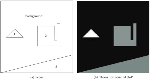
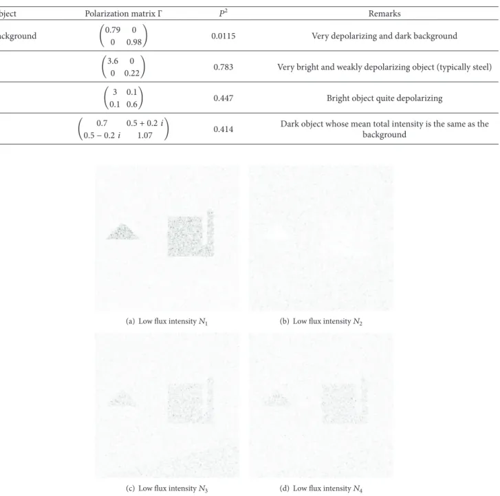
5.2. Application to Synthetic Polarimetric Images. In order to appreciate the estimation performance on polarimetric images, we consider a synthetic polarimetric image of size 512 × 512 composed of three distinct objects located on a homogeneous background depicted in Figure 4 (see also [20]). The polarimetric properties of these objects and back-ground (i.e., the covariance matrix of the Jones vector and the square DoPs) are reported in Table 5. The polarimetric low flux images generated according to this model are also represented in Figure 5 in negative colors (bright pixels corre-spond to a small number of photons, dark ones correcorre-spond to a large number of photons). Note that these images represent the values of the vector N= (𝑁1, 𝑁2, 𝑁3, 𝑁4)𝑇for each pixel. The square DoP of each pixel x(𝑖,𝑗)(for𝑖, 𝑗 = 1, . . . , 512) has been estimated from vectors belonging to windows of size 𝑛 = 15 × 15 centered around the pixel of coordinates (𝑖, 𝑗) in
log 10 MSE −1 −1.5 −2 −2.5 −3 −3.5 −4 1 1.5 2 2.5 3 3.5
log10number of pixels
ML 3D Asympt. ML 3D ML 2D Asympt. ML 2D (a) MatrixΓ2 ML 3D Asympt. ML 3D ML 2D Asympt. ML 2D log 10 MSE −2 −2.5 −3 −3.5 −4 −4.5 −5 1 1.5 2 2.5 3 3.5
log10number of pixels
(b) MatrixΓ8
Figure 3: log MSE of the estimated square DoP𝑃2using2 or 3 intensity images versus the logarithm of the sample size for the matrices (a) Γ2and (b)Γ8under high flux assumption (ML: maximum likelihood estimators, Asympt.: theoretical asymptotic value of the log MSE for a
given estimator).
2
3 1
Background
(a) Scene (b) Theoretical squared DoP
Figure 4: Composition of the scene used to generate synthetic polarimetric low flux images and associated theoretical squared DoP.
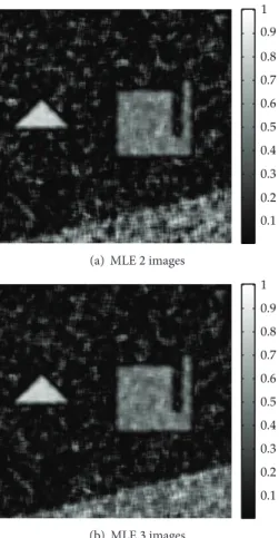
the analyzed image. The estimated square DoPs are depicted in Figures 6(a) and 6(b) for the MLEs using 2 and 3 images, respectively. One can see that the ML method for 3 images gives more homogeneous results on each object than the ML method derived for 2 images. This result confirms that the MLE using 3 images performs better than the MLE using only 2 images. However, the polarimetric properties of a scene can be clearly recovered with 2 or 3 low flux images.
5.3. Estimation Results on Real-Word Polarimetric Images. Finally, the ML estimator based on three images is applied on real polarimetric data. These images are acquired by using a laser as a coherent illumination source. The scene consists of two disks. The first one, intended to provide low DoP, is a grey diffuse material (left object in Figure 7). The second
one is made of sand blasted aluminium providing high DoP (right object in Figure 7). Due to the experimental conditions, the measured intensities are quite low. As a consequence, these intensities are assumed to be distributed according to an NMD. The intensity images corresponding to𝑁1,𝑁2,𝑁3, and 𝑁4 are depicted in Figure 7. The interested reader is invited to read [20] for more details on these data. It is important to note that the two disks exhibit the similar level of total reflectivity𝑁1+ 𝑁2and can hardly be distinguished without a polarimetric processing.
Figure 8 shows the ML estimates of the square DoPs𝑃2 for3 images and an estimation window of size 𝑛 = 9×9 pixels. As expected, the values of the estimates are quite different on each disk: quite higher on the metal than on the plastic disk. This result is in good agreement with the theoretical
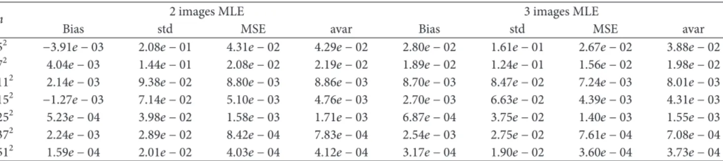
Table 3: Simulation results for the estimation of𝑃2using 2 or 3 images, obtained from1000 Monte-Carlo runs (matrix Γ2).
𝑛 2 images MLE 3 images MLE
Bias std MSE avar Bias std MSE avar
52 9.03𝑒 − 02 2.49𝑒 − 01 7.01𝑒 − 02 1.02𝑒 − 01 1.20𝑒 − 01 2.20𝑒 − 01 6.27𝑒 − 02 8.15𝑒 − 02 72 5.10𝑒 − 02 1.97𝑒 − 01 4.13𝑒 − 02 5.21𝑒 − 02 7.04𝑒 − 02 1.69𝑒 − 01 3.36𝑒 − 02 4.16𝑒 − 02 112 2.60𝑒 − 02 1.39𝑒 − 01 2.01𝑒 − 02 2.11𝑒 − 02 3.22𝑒 − 02 1.14𝑒 − 01 1.39𝑒 − 02 1.68𝑒 − 02 152 7.68𝑒 − 03 1.02𝑒 − 01 1.04𝑒 − 02 1.14𝑒 − 02 1.59𝑒 − 02 8.48𝑒 − 02 7.43𝑒 − 03 9.05𝑒 − 03 252 −7.42𝑒 − 04 6.25𝑒 − 02 3.90𝑒 − 03 4.09𝑒 − 03 2.16𝑒 − 03 5.36𝑒 − 02 2.87𝑒 − 03 3.26𝑒 − 03 372 −5.19𝑒 − 04 4.32𝑒 − 02 1.87𝑒 − 03 1.87𝑒 − 03 6.87𝑒 − 05 3.79𝑒 − 02 1.44𝑒 − 03 1.49𝑒 − 03 512 9.49𝑒 − 04 3.23𝑒 − 02 1.04𝑒 − 03 9.82𝑒 − 04 1.20𝑒 − 03 2.86𝑒 − 02 8.18𝑒 − 04 7.83𝑒 − 04
Table 4: Simulation results for the estimation of𝑃2using 2 or 3 images, obtained from1000 Monte-Carlo runs (matrix Γ8).
𝑛 2 images MLE 3 images MLE
Bias std MSE avar Bias std MSE avar
52 −3.91𝑒 − 03 2.08𝑒 − 01 4.31𝑒 − 02 4.29𝑒 − 02 2.80𝑒 − 02 1.61𝑒 − 01 2.67𝑒 − 02 3.88𝑒 − 02 72 4.04𝑒 − 03 1.44𝑒 − 01 2.08𝑒 − 02 2.19𝑒 − 02 1.89𝑒 − 02 1.24𝑒 − 01 1.56𝑒 − 02 1.98𝑒 − 02 112 2.14𝑒 − 03 9.38𝑒 − 02 8.80𝑒 − 03 8.86𝑒 − 03 8.70𝑒 − 03 8.47𝑒 − 02 7.24𝑒 − 03 8.01𝑒 − 03 152 −1.27𝑒 − 03 7.14𝑒 − 02 5.10𝑒 − 03 4.76𝑒 − 03 2.70𝑒 − 03 6.63𝑒 − 02 4.39𝑒 − 03 4.31𝑒 − 03 252 5.23𝑒 − 04 3.98𝑒 − 02 1.58𝑒 − 03 1.71𝑒 − 03 6.87𝑒 − 04 3.75𝑒 − 02 1.40𝑒 − 03 1.55𝑒 − 03 372 2.24𝑒 − 03 2.89𝑒 − 02 8.42𝑒 − 04 7.83𝑒 − 04 2.54𝑒 − 03 2.75𝑒 − 02 7.61𝑒 − 04 7.08𝑒 − 04 512 1.59𝑒 − 04 2.01𝑒 − 02 4.03𝑒 − 04 4.12𝑒 − 04 3.17𝑒 − 04 1.90𝑒 − 02 3.60𝑒 − 04 3.73𝑒 − 04
properties of the considered material. This emphasizes the interest in considering efficient estimators based on NMDs for polarimetric images.
Appendix
Proofs of the Theorems
Proof of Theorem 1. The set of affine polynomials with real coefficients and variables (𝑧1, . . . , 𝑧𝑛) is a vector space of dimension 2𝑛 spanned by the basis (z𝑇)𝑇∈P𝑛. The set of polynomials (z𝑇∏𝑡∈[𝑛]\𝑇(1 − 𝑎𝑡𝑧𝑡))𝑇∈P
𝑛 is another basis of
this vector space. The proof of the theorem is obtained by expressing the coefficients of 𝐴𝑛 in this latter basis. Considering the expansion
𝐴𝑛(𝑧1, . . . , 𝑧𝑛) = 𝑑𝑛 0∏ 𝑖∈[𝑛](1 − 𝑎𝑖𝑧𝑖) − ∑ 𝑇∈P∗ 𝑛 𝑑𝑛 𝑇z𝑇 ∏ 𝑖∈[𝑛]\𝑇(1 − 𝑎𝑖𝑧𝑖) , (A.1)
the following results can be obtained.
(1) Substituting z= 0 in (A.1) leads to 𝑑𝑛0= 1.
(2) Substituting z𝑖 = (𝛿𝑖(1), . . . , 𝛿𝑖(𝑛)) in (A.1), where 𝛿𝑖(𝑗) = 1 if 𝑖 = 𝑗 and 𝛿𝑖(𝑗) = 0 else leads to
1 − 𝑎𝑖= 1 − 𝑎𝑖− 𝑑𝑛{𝑖}, (A.2)
or equivalently 𝑑𝑛
{𝑖} = 0, 𝑖 ∈ [𝑛] . (A.3)
(3) Without loss of generality, if |𝑇| = 𝑘 > 1, the coefficients 𝑑𝑛𝑇can be computed for𝑇 = {1, . . . , 𝑘}. Indeed, consider a permutation 𝜎 such that 𝑇 = {𝜎(1), . . . , 𝜎(𝑘)}. If 𝑑𝑛
{1,...,𝑘} = 𝑓({𝑎𝑆}𝑆∈P∗
𝑘), we have
𝑑𝑛
𝑇= 𝑓({𝑎𝜎(𝑆)}𝑆∈P∗
𝑘). Using the relation
1 − 𝐴𝑛(𝑧1, . . . , 𝑧𝑛−1, 0) = ∑ 𝑇∈P∗ 𝑛−1 𝑎𝑇𝑧𝑇 = 1 − 𝐴𝑛−1(𝑧1, . . . , 𝑧𝑛−1) , (A.4) the expansion 𝐴𝑛(𝑧1, . . . , 𝑧𝑛) = ∏ 𝑖∈[𝑛](1 − 𝑎𝑖𝑧𝑖) − ∑ 𝑇∈P∗ 𝑛,|𝑇|⩾2 𝑑𝑛 𝑇z𝑇 ∏ 𝑖∈[𝑛]\𝑇(1 − 𝑎𝑖𝑧𝑖) , (A.5)
yields for any𝑘 < 𝑛, 𝑑𝑛
[𝑘]= 𝑑𝑛−1[𝑘]. (A.6)
In order to determine𝑑𝑛[𝑛], we can assume𝑎𝑖 /== 0, 𝑖 ∈ [𝑛] and substitute 𝑧𝑖 = 1/𝑎𝑖,𝑖 ∈ [𝑛] in (A.5). The
following result is obtained 1 − 𝑛 − ∑ 𝑇∈P∗𝑛,|𝑇|⩾2 𝑎𝑇 𝑎𝑇 = − 𝑑 𝑛 𝑇 𝑎[𝑛], (A.7)
Table 5: Polarimetric properties of elements that compose the scene displayed in Figure 4.
Object Polarization matrixΓ 𝑃2 Remarks
Background (0.79 0
0 0.98) 0.0115 Very depolarizing and dark background
1 (3.6 00 0.22) 0.783 Very bright and weakly depolarizing object (typically steel) 2 ( 3 0.10.1 0.6) 0.447 Bright object quite depolarizing
3 ( 0.70.5 − 0.2 𝑖 0.5 + 0.2 𝑖1.07 ) 0.414 Dark object whose mean total intensity is the same as the background
(a) Low flux intensity𝑁1 (b) Low flux intensity𝑁2
(c) Low flux intensity𝑁3 (d) Low flux intensity𝑁4
Figure 5: Synthetic intensity images (negative colors) for the scene depicted in Figure 4 and described in Table 5.
hence 𝑑𝑛[𝑛]= [ [(𝑛 − 1) +𝑇∈P∑∗𝑛,|𝑇|⩾2 𝑎𝑇 𝑎𝑇] ]𝑎 [𝑛] = ∑ 𝑇∈P∗ 𝑛,|𝑇|⩾2 𝑎𝑇𝑎[𝑛]\𝑇+ (𝑛 − 1) 𝑎[𝑛]. (A.8)
Proof of Theorem 3. The relation (10) leads to [𝐴𝑛(z)]−𝜆= (1 − 𝑄𝑛( 𝑧1 − 𝑎1 1𝑧1, . . . , 𝑧𝑛 1 − 𝑎𝑛𝑧𝑛)) −𝜆 × [∏𝑛 𝑖=1(1 − 𝑎𝑖𝑧𝑖)] −𝜆 = ( ∑ 𝛼∈N𝑛𝑐𝛼(𝜆, 1 − 𝑄𝑛) ( z 1− az) 𝛼 )
0.1 0.2 0.3 0.4 0.5 0.6 0.7 0.8 0.9 1
(a) MLE2 images
0.1 0.2 0.3 0.4 0.5 0.6 0.7 0.8 0.9 1 (b) MLE3 images
Figure 6: Estimates of𝑃2using 2 or 3 low flux intensity images for the synthetic polarimetric images for an estimation window of size 𝑛 = 15 × 15. MLE: maximum likelihood estimator.
× [∏𝑛 𝑖=1(1 − 𝑎𝑖𝑧𝑖)] −𝜆 = ( ∑ 𝛼∈N𝑛𝑐𝛼(𝜆, 1 − 𝑄𝑛) z 𝛼(1 − az)−(𝜆1+𝛼)) = ∑ 𝛼∈N𝑛𝑐𝛼(𝜆, 1 − 𝑄𝑛) z 𝛼( ∑ 𝛽∈N𝑛(𝜆1 + 𝛼)𝛽 a𝛽z𝛽 𝛽! ) = ∑ 𝛼∈N𝑛𝛽∈N∑𝑛𝑐𝛼(𝜆, 1 − 𝑄𝑛) ((𝜆1 + 𝛼)𝛽 a𝛽 𝛽! )z𝛼+𝛽 = ∑ 𝛾∈N𝑛( ∑𝛼+𝛽=𝛾𝑐𝛼(𝜆, 1 − 𝑄𝑛) (𝜆1 + 𝛼)𝛽 a𝛽 𝛽! )z𝛾 (A.9)
which proves (15). Straightforward computations allow us to obtain the equalities (16) and (17) from (15).
(a) Low flux intensity𝑁1
(b) Low flux intensity𝑁2
(c) Low flux intensity𝑁3
(d) Low flux intensity𝑁4
Figure 7: Real-world polarimetric intensity images of a scene composed of a plastic disk (left) and a steel disk (right).
Figure 8: Estimates of𝑃2 using the3 low flux intensity images 𝑁1,𝑁2, and𝑁3for the real polarimetric images for an estimation
window of size𝑛 = 9 × 9. “MLE”: maximum likelihood estimator.
Proof of Theorem 4. Denote ‖𝛼‖ = max𝑖=1,...,𝑛(𝛼𝑖), |𝛼| = ∑𝑛𝑖=1𝛼𝑖and introduce the notation of [6]
𝑐𝛼(𝜆, 𝑃𝑛) = ∑
𝑘∈𝐾𝛼
(𝜆)|𝑘|a 𝑘
where(𝜆)𝑘= 𝜆(𝜆+1) ⋅ ⋅ ⋅ (𝜆+𝑘−1) = Γ(𝜆+𝑘)/Γ(𝜆). By using Theorem 3, the following results can be obtained
𝑐𝛾(𝜆, 𝑃2) = ∑ 𝛼+𝛽=𝛾𝑐𝛼(𝜆, 1 − 𝑄2) (𝜆1 + 𝛼)𝛽 a𝛽 𝛽! = min(𝛾1,𝛾2) ∑ ℓ=0 (𝜆)ℓ(𝜆 + ℓ)𝛾1−ℓ(𝜆 + ℓ)𝛾2−ℓ ×(𝛾𝑎1𝛾1−ℓ𝑎𝛾22−ℓ𝑏1,2ℓ 1− ℓ)! (𝛾2− ℓ)!ℓ! = min(𝛾1,𝛾2) ∑ ℓ=0 Γ (𝜆 + ℓ) Γ (𝜆) Γ (𝜆 + 𝛾Γ (𝜆 + ℓ)1)Γ (𝜆 + 𝛾Γ (𝜆 + ℓ)2) ×(𝛾𝑎1𝛾1−ℓ𝑎𝛾22−ℓ𝑏1,2ℓ 1− ℓ)! (𝛾2− ℓ)!ℓ! = Γ (𝜆 + max (𝛾Γ (𝜆) 1, 𝛾2)) min(𝛾1,𝛾2) ∑ ℓ=0 Γ (𝜆 + min (𝛾1, 𝛾2)) Γ (𝜆) × Γ (𝜆)Γ (𝜆 + ℓ)𝑏1,2𝑙! (ℓ ∏2 𝑖=1 𝑎𝛾𝑖−ℓ 𝑖 (𝛾𝑖− ℓ)!) = (𝜆)max(𝛾1,𝛾2) min(𝛾1,𝛾2) ∑ ℓ=0 (𝜆 + ℓ)min(𝛾1,𝛾2)−ℓ (𝛾1− ℓ)! (𝛾2− ℓ)!ℓ! × 𝑎𝛾1−ℓ 1 𝑎2𝛾2−ℓ𝑏1,2ℓ . (A.11)
Proof of Theorem 6. The relation (16) with𝑄3(z) = 𝑏1,2𝑧1𝑧2+
𝑏1,3𝑧1𝑧3 + 𝑏2,3𝑧2𝑧3 + 𝑏1,2,3𝑧1𝑧2𝑧3leads to (22). By using the
trivial equality 𝑏𝑣−𝛾1+𝛽1 2,3 𝑏1,3𝑣−𝛾2+𝛽2𝑏1,2𝑣−𝛾3+𝛽3𝑏1,2,3|𝛾−𝛽|−2𝑣𝑎𝛽11𝑎2𝛽2𝑎3𝛽3 = (𝑏2,3𝑏𝑏21,3𝑏1,2 1,2,3 ) 𝑣 (∏3 𝑖=1𝑎 𝛾𝑖 𝑖 ) (𝑎𝑏1,2,3 1𝑏2,3) 𝛾1−𝛽1 × (𝑎𝑏1,2,3 2𝑏1,3) 𝛾2−𝛽2 (𝑎𝑏1,2,3 3𝑏1,2) 𝛾3−𝛽3 (A.12)
we easily obtain (23). Note that for‖𝛼‖ ⩽ 𝑣 ⩽ ⌊|𝛼|/2⌋, we have(𝜆)𝑣 = (𝜆)‖𝛼‖(𝜆 + ‖𝛼‖)𝑣−‖𝛼‖. By substituting𝛼𝑖= 𝛾𝑖− 𝛽𝑖, 𝑖 = 1, 2, 3 in (23), the last result (24) can be obtained.
Acknowledgments
The authors would like to thank G´erard Letac for fruitful discussions regarding multivariate gamma distributions and negative multinomial distributions. The Authors are also grateful to Mehdi Alouini for acquiring and providing them the polarimetric images.
References
[1] D. C. Doss, “Definition and characterization of multivariate negative binomial distribution,” Journal of Multivariate Analy-sis, vol. 9, no. 3, pp. 460–464, 1979.
[2] N. L. Johnson, S. Kotz, and N. Balakrishnan, Discrete Multivari-ate Distributions, John Wiley & Sons, New York, NY, USA, 1997. [3] F. Le Gall, “The modes of a negative multinomial distribution,” Statistics and Probability Letters, vol. 76, no. 6, pp. 619–624, 2006.
[4] R. C. Griffiths and R. K. Milne, “A class of infinitely divisible multivariate negative binomial distributions,” Journal of Multi-variate Analysis, vol. 22, no. 1, pp. 13–23, 1987.
[5] S. K. Bar-Lev, D. Bshouty, P. Enis, G. Letac, I. L. Lu, and D. Richards, “The diagnonal multivariate natural exponential fam-ilies and their classification,” Journal of Theoretical Probability, vol. 7, no. 4, pp. 883–929, 1994.
[6] P. Bernardoff, “Which negative multinomial distributions are infinitely divisible?” Bernoulli, vol. 9, no. 5, pp. 877–893, 2003. [7] F. Chatelain, S. Lambert-Lacroix, and J. Y. Tourneret, “Pairwise
likelihood estimation for multivariate mixed Poisson models generated by gamma intensities,” Statistics and Computing, vol. 19, no. 3, pp. 283–301, 2009.
[8] C. Brosseau, Fundamentals of Polarized Light—A Statistical Approach, John Wiley & Sons, New York, NY, USA, 1998. [9] J. S. Lee and E. Pottier, Polarimetric Radar Imaging: From Basics
to Applications, Optical Science and Engineering, Taylor & Francis, London, UK, 2009.
[10] S. Huard, Polarization of LightStatistical Optics, John Wiley & Sons, New York, NY, USA, 1997.
[11] H. Mott, Remote Sensing With Polarimetric Radar, John Wiley & Sons, New York, NY, USA, 2007.
[12] R. Shirvani, M. Chabert, and J. Y. Tourneret, “Ship and oil-spill detection using the degree of polarization in linear and hybrid/compact dual-pol SAR,” IEEE Journal of Selected Topics in Applied Earth Observations and Remote Sensing, vol. 5, no. 3, pp. 885–892, 2012.
[13] R. C. Jones, “A new calculus for the treatment of optical systems V. A more general formulation and description of another calculus,” vol. 37, no. 2, pp. 107–110, 1947.
[14] E. Wolf, “Coherence properties of partially polarized electro-magnetic radiation,” Il Nuovo Cimento, vol. 13, no. 6, pp. 1165– 1181, 1959.
[15] J. Goodman, Statistical Optics, John Wiley & Sons, New York, NY, USA, 1985.
[16] J. Fade, M. Roche, and P. R´efr´egier, “Precision of moment-based estimation of the degree of polarization in coherent imagery without polarization device,” Journal of the Optical Society of America A, vol. 25, no. 2, pp. 483–492, 2008.
[17] J. Fade, P. R´efr´egier, and M. Roche, “Estimation of the degree of polarization from a single speckle intensity image with photon noise,” Journal of Optics A, vol. 10, no. 11, Article ID 115301, 2008. [18] P. R´efr´egier, M. Roche, and F. Goudail, “Cramer-Rao lower bound for the estimation of the degree of polarization in active coherent imagery at low photon levels,” Optics Letters, vol. 31, no. 24, pp. 3565–3567, 2006.
[19] M. Roche, J. Fade, and P. R´efr´egier, “Parametric estimation of the square degree of polarization from two intensity images degraded by fully developed speckle noise,” Journal of the Optical Society of America A, vol. 24, no. 9, pp. 2719–2727, 2007.
[20] F. Chatelain, J. Y. Tourneret, M. Roche, and M. Alouini, “Estimating the polarization degree of polarimetric images in coherent illumination using maximum likelihood methods,” Journal of the Optical Society of America A, vol. 26, no. 6, pp. 1348–1359, 2009.
[21] W. B. Sparks and D. J. Axon, “Panoramic polarimetry data analysis,” Publications of the Astronomical Society of the Pacific, vol. 111, no. 764, pp. 1298–1315, 1999.
[22] A. Ferrari, G. Letac, and J. Y. Tourneret, “Multivariate mixed poisson distributions,” in Proceedings of the EUSIPCO-04, F. Hlawatsch, G. Matz, M. Rupp, and B. Wistawel, Eds., pp. 1067– 1070, Vienna, Austria, September 2004.
[23] F. Chatelain, Lois statistiques multivariees pour le traitement de l’image [Ph.D. thesis], Institut National Polytechnique de Toulouse, Toulouse, France, 2007.