HAL Id: inserm-00585285
https://www.hal.inserm.fr/inserm-00585285
Submitted on 10 May 2011
HAL is a multi-disciplinary open access
archive for the deposit and dissemination of
sci-entific research documents, whether they are
pub-lished or not. The documents may come from
teaching and research institutions in France or
abroad, or from public or private research centers.
L’archive ouverte pluridisciplinaire HAL, est
destinée au dépôt et à la diffusion de documents
scientifiques de niveau recherche, publiés ou non,
émanant des établissements d’enseignement et de
recherche français ou étrangers, des laboratoires
publics ou privés.
GPU Accelerated High Intensity Ultrasound Acoustical
Power Computation
Tingting Gu, Hui Tang, Xudong Bao, Jean-Louis Dillenseger
To cite this version:
Tingting Gu, Hui Tang, Xudong Bao, Jean-Louis Dillenseger. GPU Accelerated High Intensity
Ultra-sound Acoustical Power Computation. 8th International Symposium on Biomedical Imaging (ISBI’11),
Mar 2011, United States. pp.17-20. �inserm-00585285�
GPU ACCELERATED HIGH INTENSITY ULTRASOUND ACOUSTICAL POWER
COMPUTATION
Gu Tingting
⋆†Tang Hui
†‡Bao Xudong
†‡Dillenseger Jean-Louis
‡∗⋄⋆
Department of Biomedical Engineering, Southeast University, Nanjing 210096
†Laboratory of Image Science and Technology, Southeast University, Nanjing 210096
‡
Centre de Recherche en Information Biom´edicale Sino-Franc¸ais (CRIBs)
∗INSERM, U642, Rennes, F-35000, France
⋄
Universit´e de Rennes 1, LTSI, Rennes, F-35000, France
ABSTRACT
The simulation of the hepatocellular carcinoma therapy effects is often used for the intervention planning. As the physical-based model of the simulation is very time-consuming, the speed of this method becomes an obstacle during the clinical application simulation. In order to accel-erate the simulation, a GPU-based (Graphic Processing Unit) acceleration method of the pressure field estimation is pro-posed in this paper. The results demonstrate that the propro-posed acceleration method can solve the time-consuming problem.
Index Terms— high intensity ultrasound therapy,
simu-lation, interstitial therapy, GPU
1. INTRODUCTION
High intensity ultrasound interstitial method is an alternative for the treatment of Hepatocellular carcinoma (HCC). This technique seems to be more advantageous for the control of depth and direction [1]. During the clinical application, an ef-ficient simulation of the effects of treatment should be made at the pre-operative stage. A first computer simulation tool for high energy ultrasound interstitial therapy assumed that the tissues are homogeneous with physical properties invari-ant during the treatment [1]. But this assumption limited the accuracy and realism of the model. Garnier et al. introduced a more accurate model which takes into account the variation in time and temperature of the tissue attenuation coefficient [2]. This model is divided into several steps: 1) simulation of the pressure field generated by the transducer, 2) estimation of the temperature evolution over time and 3) estimation of the induced necrosis. In this framework, the pressure field sim-ulation is one of the major points. The pressure field can be exactly estimated on the basis of Rayleigh integrals [1]. As the computation of Rayleigh integral is very time-consuming,
This work is part of the French MULTIP project supported by an ANR Grant (ANR-09-TECS-011-06).
the speed of the implementation of the model becomes an ob-stacle for its use as pre-operative planning of the clinical ap-plication. In order to accelerate the estimation, Dillenseger et al. made several simplifications on the model [3]. However, the acceleration is still not satisfying and it brings high er-rors at the same time. To further accelerate the estimation of pressure field, we propose a GPU-based method. As the com-putation of each point in the pressure field is relatively inde-pendent and parallel, we think that it can be accelerated by the programmable graphics hardware due to its parallel computa-tion ability. In this paper we will try to estimate the speedup efficiency and errors of this GPU-based method compared to the traditional methods computed on CPU.
2. METHOD
2.1. Ultrasound device
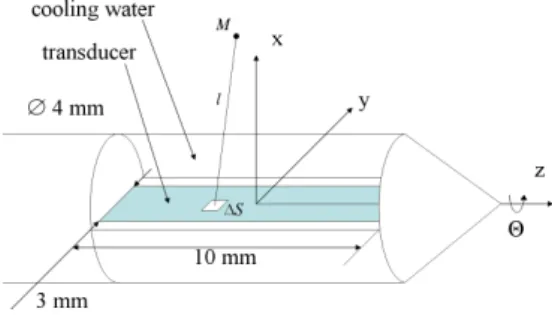
The modeled therapeutic ultrasound device is composed of a small planar ultrasonic monoelement transducer encapsulated in a cylindrical interstitial applicator (Fig.1) [2]. The trans-ducer is air-backed, so that the ultrasound is only propagated forward. The front face is cooled by water.
2.2. Pressure computation
The estimation of pressure field is a key point of the effect simulation. Numerical methods for estimating the pressure field can take into account the nonlinear propagation of high intensity waves or remain purely linear. Because of the rel-atively low power of the input transducer pressure and the non-focusing geometry of the probe, the propagation can be considered linear [4] and the pressure field can be exactly computed on the basis of the Rayleigh integral with O’Neil’s hypotheses [1]. The transducer surface S is sampled into el-ements of surface ∆S which size is negligible in comparison with wavelength λ (∆S < (λ/7)2). Each surface element
can be considered as a single radial emitter. A location M and one element of surface ∆S are connected by a straight segment of length l sampled into elements ∆l as shown in Fig.1. The pressure at M is given by the discrete version of the Rayleigh integral:
p(M ) = ∑ S jp0 λ∆S exp−jkl l exp −f∑l i=1αi∆l (1) with p0the pressure at the transducer surface (Pa), k the
wave number (2π/λ), f the transducer frequency (Hz) and αi
the tissue attenuation coefficient at location i along the line segment ∆SM (Np· m−1· MHz−1).
2.3. Software simplifications
This two fold integration of (1) (over the surface of the trans-ducer and along the segment ∆SM ) is very computation in-tensive, especially when the tissue attenuation coefficients αi
are inhomogeneous over the volume and are temperature de-pendent [5]. Dillenseger et al. [3] made several reasonable simplifications for the computation of Rayleigh integral. In the following part, we will briefly describe these methods. As
αican be taken into account in 4 different manners, the
com-putation varies greatly in different conditions.
2.3.1. Adaptive sampling
As the pressure in the regions near the transducer presents larger variation than those more distant, adaptive sampling of the volume could be used to accelerate computation. An adaptive sampling of the points M over the volume is used. The pressure is first computed on one sample point every 8 sample points along each direction. The rule is: if the pressure values computed on adjacent sampled points is bellow than a first threshold P1 = max(p(M ))/2 and if the difference
between these two pressure values is lower than a second ad hoc set threshold P2= max(p(M ))/100, the pressure on the
intermediate sample point is computed by linear interpolation, otherwise by Rayleigh integral (1).
2.3.2. Segments coherence
Adjacent ∆SM segments share almost the same attenuation properties. For a patch A of nine adjacent connected trans-ducer surface element ∆S, the exp−f∑li=1αi∆lattenuation
term of (1) is computed for only the ∆SM segment which originates from the central surface element of A and then ap-plied to the 8 other segments which originate from A. There-fore, (1) can be rewritten as:
p(M ) = ∑ S′ jp0 λ∆S ( ∑ A exp−jklp lp ) exp−f∑lci=1αi∆lc (2) with S′ the central surface elements of all patches A, lp
the length from point M to each point of patch A and lcthe
length from point M to the center of patch A.
2.3.3. Mean attenuation
A much simpler method is to calculate the attenuation integra-tion only one time. The attenuaintegra-tion is computed once along the ray from the center O of the transducer to the point M . On this condition, (1) can be rewritten as:
p(M ) = ( ∑ S jp0 λ∆S exp−jkl l ) exp−f∑loi=1αi∆lo (3) with lothe length from point M to center of transducer O.
2.3.4. Constant attenuation
When the tissues are assumed to be homogeneous, the prop-agation of a wave from one element of surface ∆S to M is carried through 2 media: the cooling water of the transducer (α1 ≈ 0, l1) and the tissues (α2, l2). Because of the
trans-ducer geometry, l1 and l2 can be estimated analytically and
(1) can therefore be simplified to:
p(M ) = ∑ S jp0 λ∆S exp−jkl l exp −fα2l2 (4) This assumption allows a relatively fast power field com-putation but to the detriment of realism.
3. IMPLEMENTATION ON GPU
Analyzing the Rayleigh integral, it is obvious that the bot-tleneck of the implementation of the algorithm is the large amount of parallel integral computation. The improvements brought by the different simplifications proposed in [3] are not satisfying considering the limited speedup as well as high errors.
In recent years, the rapid development of GPU and its unique parallel feature make it a new and brilliant tool for scientific computation. Parallelism could be performed on two level: 1) on a more lower level to estimate the pressure on one location M by the parallel pressure computation of each ray (from one element of surface ∆S to M ) and 2) on a more higher level by the parallel computation of the pressure at each M of the volume. Moreover, the exp−f∑li=1αi∆l
attenuation term is similar to the compositing equation used in volume rendering [6], which inspires us to use GPU for acceleration. Therefore, we introduce GPU for accelerating Rayleigh integral.
We will only consider the computation of the pressure on one location M . In order to decompose the overall equation, the real part prand imaginary part piof the pressure induced
by each ray are computed separately. Then the total pressure of (1) is achieved according to:
p(M ) = Q v u u t(∑ S pr )2 + ( ∑ S pi )2 (5) where: Q = p0 λ∆S; pr= cos(−kl) l exp−f ∑l i=1αi∆land pi=sin(−kl)l exp−f ∑l i=1αi∆l.
The program flow chart is shown in Fig. 2. First the sampled points of the transducer surface are transferred to the vertex processor of the programmable graphics hardware pipeline. After rasterization, the sampled points are sent into the fragment processor. Meanwhile, a 3D texture for storing the attenuation coefficients of the whole volume, the location of point M and other variables for computing prand pi are
transferred from CPU application into the fragment processor. Then, the fragment shader (program coded in GLSL -OpenGL Shading Language- for fragment processor) is ex-ecuted in parallel by fragment processor to compute pr and pi. As GLSL is based on C and C++ syntax, the source
pro-gram of the fragment shader can be designed similarly with that in C++ function except for transforming texture coordi-nates to Cartesian coordicoordi-nates at first. At the end of fragment shader, prand pi for each ray are stored respectively in two
frame buffers, fetched by two 2D Textures and transferred into CPU application. Finally the overall pressure at point
M is achieved according to (5) in CPU program. During the
whole process above, only the computation of pr and pi is
parallel and run on GPU. For the pressure computation of each sample point M , the process is also parallel. However, this parallel computation depends on parallel computation of each ray. This dependence makes it impossible to run on GPU.
Fig. 2. Program flow chart of GPU-based Rayleigh integral.
4. RESULTS
4.1. Evaluation protocol
The comparison of the results obtained by the several sim-plification methods is performed with the following proto-col. We simulate the pressure field p induced by a 5MHz transducer (Fig.1) with an acoustical intensity of 40W/cm2. The size of transducer is 3mm× 9mm. It has been shown in [3] that a ∆S = (λ/4)2 gives a good compromise be-tween speedup and accuracy. The transducer is centered in a 80mm× 80mm × 24mm volume which is regularly sam-pled with a 0.4mm sampling step on 201× 201 × 61 points. The pressure field simulated by (1) (we will call it later brute-force simulation) only with CPU will be considered as reference. Several measurements are performed to compare the pressure field obtained by the several methods to the ref-erence one or to compare GPU and CPU: the mean absolute error (labeled as mean abs. error), the mean relative error (mean rel. error), the computation time and the acceleration rate (acc. rate) which is the ratio of the computation time obtained by a simplified or a GPU-based method to the com-putation time of the reference method.
We have evaluated the whole implementation on a HP Z800 workstation equipped with a Intel Xeon 5504 2.00 GHz CPU, with 1.99 GB RAM and a NVIDIA Quadro FX 5600 (1536 MB) video card.
4.2. Results
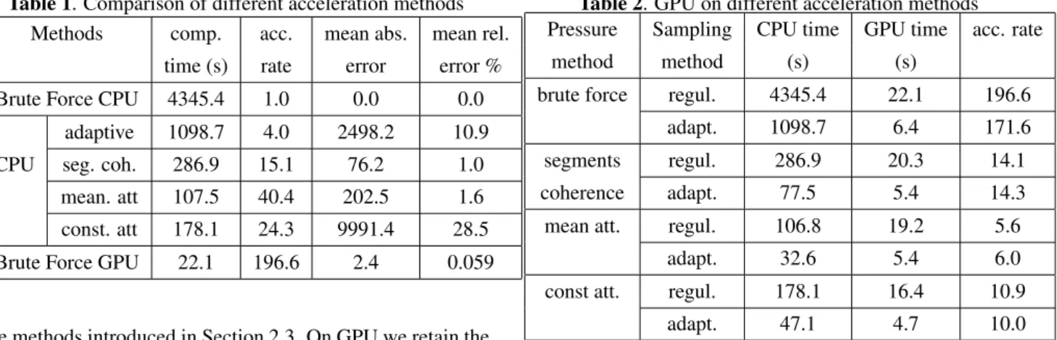
The comparison of different methods is shown on Table 1. The four CPU simplification methods are corresponding to
Table 1. Comparison of different acceleration methods Methods comp. acc. mean abs. mean rel.
time (s) rate error error % Brute Force CPU 4345.4 1.0 0.0 0.0
adaptive 1098.7 4.0 2498.2 10.9 CPU seg. coh. 286.9 15.1 76.2 1.0
mean. att 107.5 40.4 202.5 1.6 const. att 178.1 24.3 9991.4 28.5 Brute Force GPU 22.1 196.6 2.4 0.059
the methods introduced in Section 2.3. On GPU we retain the implementation without any simplifications.
From Table 1, we can see that among the four simplifi-cation methods, the fastest is the mean attenuation method. However, with the fastest computation speed, it brings big er-rors. The error of the second simplification method (labeled as seg. coh.) is the smallest, but its acceleration rate is not satisfying. From this table, we can clearly see that the perfor-mance of GPU-based method is the best. The speedup ability is considerable while the computation error is tiny. Compared to the results of the other simplification methods, this compu-tation error even can be neglected. This GPU acceleration is even more significant when more rays are taken into account. For example, when the size of ∆S = (λ/10)2, the
compu-tation times of the two brute force methods are respectively 27507.5s and 60.3s (acc. rate = 456). The reason is that when the size of ∆S is smaller there are more parallel computa-tion to be applied on GPU and therefore much more speedup brought by GPU.
GPU can also be used for implementing the acceleration methods as mentioned in Section 2.3. We tested the regular and adaptive volume sampling on all the methods. The com-parison of these acceleration methods is shown on Table 2. The errors between a CPU-based and a GPU-based method is negligible. The acceleration rate between CPU and GPU computation differs between the several methods. We can see that the computation of the attenuation term takes the main benefits of the GPU computation. We draw a conclusion that to what extend an algorithm could be accelerated by GPU de-pends both on parallelism of the algorithm and computation cost of each parallel process.
5. CONCLUSION
In this paper we proposed a GPU-based acceleration method for the acoustical power computation during the planning of ultrasound therapy. The new method takes advantage of the parallel feature of the algorithm and the parallel computation power of GPU. The proposed method achieves considerable speed-up comparing to the traditional method while
remain-Table 2. GPU on different acceleration methods Pressure Sampling CPU time GPU time acc. rate
method method (s) (s)
brute force regul. 4345.4 22.1 196.6 adapt. 1098.7 6.4 171.6 segments regul. 286.9 20.3 14.1 coherence adapt. 77.5 5.4 14.3 mean att. regul. 106.8 19.2 5.6
adapt. 32.6 5.4 6.0 const att. regul. 178.1 16.4 10.9
adapt. 47.1 4.7 10.0
ing high computation accuracy. The acceleration is much more considerable when the part computed on GPU (e.g. pr
and piin this program) is very time consuming. However, the
parallel pressure computation at different space location M was not applied because its dependence on the parallel pres-sure computation of each ray. Further study could be focused on deliberately designing the program to make better use of the GPU parallel computation ability.
6. REFERENCES
[1] C. Lafon, F. Prat, J. Y. Chapelon, F. Gorry, J. Margonari, Y. Theillere, and D. Cathignol, “Cylindrical thermal co-agulation necrosis using an interstitial applicator with a plane ultrasonic transducer: in vitro and in vivo experi-ments versus computer simulations,” Int J Hyperthermia, vol. 16, no. 6, pp. 508–22, 2000.
[2] C. Garnier, C. Lafon, and J.-L. Dillenseger, “3D model-ing of the thermal coagulation necrosis induced by an in-terstitial ultrasonic transducer,” IEEE Trans Biomed Eng, vol. 55, no. 2, pp. 833–7, 2008.
[3] J.-L. Dillenseger and C. Garnier, “Acoustical power com-putation acceleration techniques for the planning of ultra-sound therapy,” in 5th IEEE International Symposium on
Biomedical Imaging, Paris, 2008, pp. 1203–1206.
[4] F. A. Duck, “Nonlinear acoustics in diagnostic ultra-sound,” Ultrasound Med Biol, vol. 28, no. 1, pp. 1–18, 2002.
[5] C. A. Damianou, N. T. Sanghvi, F. J. Fry, and R. Maass-Moreno, “Dependence of ultrasonic attenuation and ab-sorption in dog soft tissues on temperature and thermal dose,” J Acoust Soc Am, vol. 102, no. 1, pp. 628–34, 1997.
[6] M. Levoy, “Display of surfaces from volume data,” IEEE