Publisher’s version / Version de l'éditeur:
Vous avez des questions? Nous pouvons vous aider. Pour communiquer directement avec un auteur, consultez
la première page de la revue dans laquelle son article a été publié afin de trouver ses coordonnées. Si vous n’arrivez pas à les repérer, communiquez avec nous à [email protected].
Questions? Contact the NRC Publications Archive team at
[email protected]. If you wish to email the authors directly, please see the first page of the publication for their contact information.
https://publications-cnrc.canada.ca/fra/droits
L’accès à ce site Web et l’utilisation de son contenu sont assujettis aux conditions présentées dans le site LISEZ CES CONDITIONS ATTENTIVEMENT AVANT D’UTILISER CE SITE WEB.
Proceedings of the 16th European Conference of Machine Learning
[Proceedings], 2005
READ THESE TERMS AND CONDITIONS CAREFULLY BEFORE USING THIS WEBSITE.
https://nrc-publications.canada.ca/eng/copyright
NRC Publications Archive Record / Notice des Archives des publications du CNRC :
https://nrc-publications.canada.ca/eng/view/object/?id=f0b7a37b-d7c5-470c-b6e5-eb7321281478
https://publications-cnrc.canada.ca/fra/voir/objet/?id=f0b7a37b-d7c5-470c-b6e5-eb7321281478
NRC Publications Archive
Archives des publications du CNRC
This publication could be one of several versions: author’s original, accepted manuscript or the publisher’s version. / La version de cette publication peut être l’une des suivantes : la version prépublication de l’auteur, la version acceptée du manuscrit ou la version de l’éditeur.
Access and use of this website and the material on it are subject to the Terms and Conditions set forth at
Severe Class Imbalance: Why Better Algorithms Aren't the Answer
National Research Council Canada Institute for Information Technology Conseil national de recherches Canada Institut de technologie de l'information
Severe Class Imbalance: Why Better
Algorithms Aren't the Answer *
Drummond, C., and Holte, R.C.
October 2005
* published in the Proceedings of the 16th European Conference of Machine Learning. Porto, Portugal. October 3-7, 2005. NRC 48258.
Copyright 2005 by
National Research Council of Canada
Permission is granted to quote short excerpts and to reproduce figures and tables from this report, provided that the source of such material is fully acknowledged.
Severe Class Imbalance: Why Better Algorithms
Aren’t the Answer
Chris Drummond1
and Robert C. Holte2 1
Institute for Information Technology, National Research Council Canada, Ottawa, Ontario, Canada, K1A 0R6 [email protected]
2
Department of Computing Science, University of Alberta, Edmonton, Alberta, Canada, T6G 2E8 [email protected]
Abstract. This paper argues that severe class imbalance is not just an interesting technical challenge that improved learning algorithms will ad-dress, it is much more serious. To be useful, a classifier must appreciably outperform a trivial solution, such as choosing the majority class. Any application that is inherently noisy limits the error rate, and cost, that is achievable. When data are normally distributed, even a Bayes optimal classifier has a vanishingly small reduction in the majority classifier’s error rate, and cost, as imbalance increases. For fat tailed distributions, and when practical classifiers are used, often no reduction is achieved.
1
Introduction
Class imbalance, and the difficulties that result, has been a topic of much interest in recent years in machine learning [1]. When classes are imbalanced, existing learning algorithms often produce classifiers that do little more than predict the most common class. It seems intuitive that a practical classifier must do much better on the minority class, often the one of greatest interest, even if this means sacrificing performance on the majority class. If the overall error rate becomes worse, so the reasoning goes, then it fails to capture what practically matters and alternative measures are needed. Researchers have looked at separate error rates for positive and negative classes [2], the functional relationship between them [3] and the area under the function [4].
Although we use expected cost, we feel it is less a matter that the measure is wrong, it is more that the majority classifier is very hard to beat when classes are severely imbalanced. Differential costs may reduce the problem bur they are by no means guaranteed to eliminate it. We are not simply reiterating a com-mon observation that sometimes the majority classifier’s error rate is so small that it seems little can be done to improve on it. We are making the stronger claim that a “relative reduction” in error rate is often unachievable. We use the fraction of the majority classifier’s error rate removed because it is important to consider what success means when a trivial classifier gets only say 1% wrong. In this case, a classifier with a 0.4% error rate has an error rate reduction of 0.6, a respectable value. This is equivalent to a 20% error rate when the classes
are balanced and the majority classifier gets 50% wrong. This idea is especially intuitive when considering misclassification costs [5, 6]. The success of a classifier is how much it reduces the cost when using a trivial classifier. Even a Bayes op-timal classifier, at least as good as the majority classifier, often only has a small relative cost reduction. As imbalance increases, this becomes even smaller. For practical algorithms just performing as well as the majority classifier becomes progressively harder. Improved learning algorithms will not eliminate the prob-lem. If the application is inherently noisy, no amount of boosting, bagging or kernelizing can produce performance beyond Bayes optimal.
Our results address applications where all instances of one class have the same misclassification costs. If costs are highly non-linear, say it is enough to classify a small number instances correctly ignoring the rest, our arguments are not relevant. This may be true in some information retrieval tasks, where only a very small fraction of the positive instances are required to satisfy a query. Occasionally, a small performance gain over the majority classifier is the differ-ence between success and failure. We claim that many, if not most, classification applications are not of either type. At the very least, our own experience tells us, the type of application addressed here is common enough that the conclusions we draw should be relevant to many researchers and practitioners.
2
Visualizing the Problem
This section gives a brief introduction to cost curves [7], a way to visualize clas-sifier performance over different misclassification costs and class distributions.
The error rate of a binary classifier is a convex combination of the likelihood functions P (−|+), P (+|−), where P (L|C) is the probability that an instance of class C is labeled L and the coefficients P (+), P (−) are the class priors:
E[Error] = P (−|+) | {z } F N P(+) + P (+|−) | {z } F P P(−)
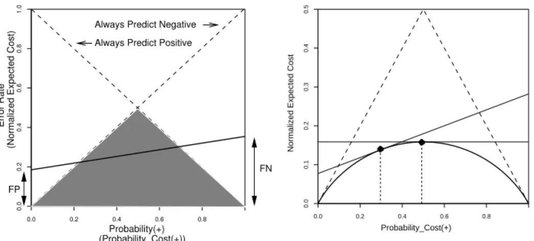
Estimates of the likelihoods are the false positive (FP) and false negative (FN) rates. A straight line, such as the one in bold in Figure 1, gives the error rate on the y-axis (ignore the axis labels in parentheses for the moment), for each possible prior probability of an instance belonging to the positive class on the x-axis. If this line is completely below another line, representing a second classifier, it has a lower error rate for every probability. If they cross, each classifier is better for some range of priors. Of particular note are the two trivial classifiers, the dashed lines in the figure. One always predicts that instances are negative, the other that instances are positive. Together they form the majority classifier, the shaded triangle in Figure 1, which predicts the most common class. The figure shows that any single classifier with a non-zero error rate will always be outperformed by the majority classifier if the priors are sufficiently skewed, therefore of little use. Even a good classifier produces too many false positives when negative examples are very common [8].
0.6 0.0 0.2 0.4 0.6 0.8 0.0 0.2 0.8 1.0 0.4 Probability(+) (Probability_Cost(+)) FN Always Predict Positive
Always Predict Negative
(Normalized Expected Cost)
Error Rate
FP
Fig. 1.Visualizing Performance
0.1 0.3 0.4 0.5 Probability_Cost(+) 0.0 0.2 0.4 0.6 0.8 0.0 0.2
Normalized Expected Cost
Fig. 2.The Cost Curve
If misclassification costs are taken into account, expected error rate is re-placed by expected cost, as defined by Equation 1. The expected cost is also a convex combination of the prior probabilities, but plotting it against the priors would produce a y-axis that no longer ranges from zero to one. The expected cost is normalized by dividing by the maximum value, given by Equation 2. The costs and priors are combined into the Probability Cost(+) on the x-axis, as in Equation 3. Applying the same normalization factor results in an x-axis that ranges from zero to one, as in Equation 4. The positive and negative Probabil-ity Cost( )’s now sum to one, as was the case with the probabilities.
E[Cost] = F N ∗ C(−|+)P (+) + F P ∗ C(+|−)P (−) (1) max(E[Cost]) = C(−|+)P (+) + C(+|−)P (−) (2) P C(+) = C(−|+)P (+) (3) N orm(E[Cost]) = F N ∗ P C(+) + F P ∗ P C(−) (4) With this representation, the axes in Figure 1 are simply relabeled, using the text in parentheses, to account for costs. Misclassification costs and class frequencies are more imbalanced the further away from 0.5, the center of the diagram. The lines are still straight. There is still a triangular shaded region, but now representing the classifier predicting the class that has the smaller expected cost. For simplicity we shall continue to refer to it as the majority classifier.
In Figure 2 the straight continuous lines are Bayes optimal classifiers for two different class frequencies or costs, indicated by the vertical dashed lines. The classifier represented by the horizontal line is optimal when the classes and costs are balanced. The second classifier is optimal when there are more nega-tive examples, or they are more costly to misclassify. If the optimal classifier is identified for every probability-cost value and a point put on each line at that
value, as indicated by the black dots in Figure 2, the set of such points defines the continuous bold curve. So generally as the balance changes, there is a smooth trade-off between positives that are incorrectly classified and negatives that are incorrectly classified. Most practical learning algorithms also generate different classifiers for different priors and make a principled trade off between the num-ber of errors on the positive and negative classes. They produce similar curves, although their curves will generally be above the curve in Figure 2 because their performance will fall somewhat short of Bayes optimal.
3
Imbalance and Performance
In this section, we show that a Bayes optimal classifier performs only marginally better than a trivial classifier when there is severe imbalance. This difference is even smaller if the likelihood functions have fat tails or the classifier suboptimal.
3.1 Increasing Imbalance
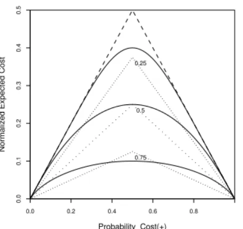
Figure 3 shows cost curves for the Bayes optimal classifier for two, unit vari-ance, normal distributions, representing the likelihood functions for two classes. The continuous curves are for 3 different distances between their means. The distances were chosen to make the relative cost reduction when the classes are balanced 0.2, 0.5 and 0.8. The series of progressively smaller triangles, the dotted lines, we call cost reduction contours. They are triangles because the majority classifier is a triangle. Each contour indicates the reduction in cost achieved by the new classifier as a fraction of the cost of using the majority classifier. For instance, the central contour, marked 0.5, indicates a reduction of one half of the cost. The continuous curves cross multiple contours indicating a decreasing relative cost reduction as imbalance increases.
0.75 0.0 0.2 0.4 0.6 0.8 0.0 0.1 0.2 0.3 0.4 0.5 Probability_Cost(+)
Normalized Expected Cost
0.25
0.5
Fig. 3.Different Separations
Normalized Expected Cost
0.00 0.02 0.04 0.06 0.08 0.00 0.01 0.02 0.03 0.04 0.05 Probability_Cost(+)
Zooming in on the lower left hand corner of Figure 3 gives Figure 4. Here negative instances are much more common than the positives, or more costly to misclassify. The upper two curves have become nearly indistinguishable from the majority classifier for ratios about 20:1. The lowest cost curve has crossed the 0.5 cost reduction contour at an imbalance of about 10:1 and crossed the 0.25 cost reduction contour at about 50:1. So even starting with a very good classifier with a 0.8 relative cost reduction when there is no imbalance (i.e. a 10% error rate), the benefit decays rapidly as imbalance increases.
3.2 Different Distributions
In this section we investigate what happens if the data are not drawn from normal distributions. We use the “power exponential” distribution, shown in Figure 5, which has a factor controlling the fatness of the tails. The bold curve is the normal distribution, this acts as the standard for tail fatness. At one extreme is the double exponential, or Laplace, distribution. At the other extreme is the uniform distribution. The double exponential distribution is relatively low in the middle and spreads out widely, giving it the fat-tails. As the factor is increased the center rises and thickens as the tails diminish. Ultimately, as we approach the uniform distribution, the tails thin out and disappear.
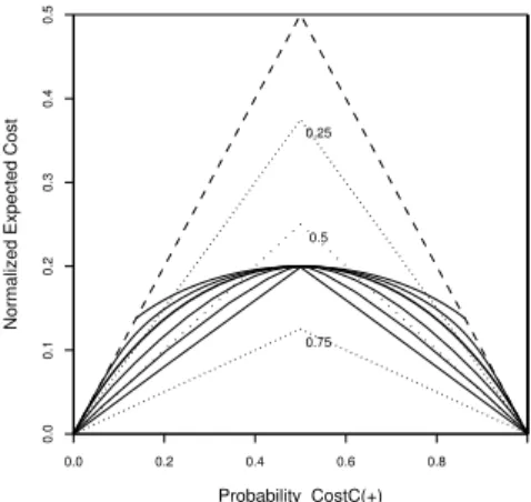
Figure 6 shows cost curves when the distributions in Figure 5 are used to define the likelihood functions for both classes. The distances between their means were chosen so that all curves have the same normalized expected cost of 0.2 when balanced. The curve for the normal distribution is the bold continuous line. Curves with fatter tails are even more sensitive to imbalance. The topmost curve is for the double exponential. It has exactly the same cost as the majority classifier when imbalance is about 8:1 or 1:8. The distributions with fatter tails than the normal distribution all have a relative cost reduction of only 0.1 if the imbalance is greater than 10:1. It is true, however, that distributions with thinner tails than the normal distribution reduce the cost proportionally more. In fact, two overlapping uniform distributions (the thinnest possible tails and the lowest continuous curve in Figure 6) have the same relative cost reduction for severe imbalance as for perfect balance.
If uniform distributions give consistent performance perhaps nominal at-tributes do as well. Uniform distributions are like a single nominal attribute with three values, the middle one is where they overlap. Suppose there are 100 positives with value A, 100 with value B and 100 negatives with value B, 100 with value C, see the top left of the Figure 7. Varying the imbalance produces a triangular cost curve, the same as with uniform distributions. But suppose some of the negative and positive classes are redistributed such that values A and C no longer contain just one class, shown at the top right of Figure 7. This produces the upper bold curve where the classifier has the same performance as the majority classifier for ratios as low as 6:1.
x 0.3 0.4 0.5 p(x) 0.6 −4 −2 0 2 4 0.0 0.1 0.2 ExponentialDouble Normal Uniform
Fig. 5.Changing the Tails
0.75 0.0 0.2 0.4 0.6 0.8 0.0 0.1 0.2 0.3 0.4 0.5 Probability_CostC(+)
Normalized Expected Cost
0.25
0.5
Fig. 6.Different Distributions
0 0.0 0.2 0.4 0.6 0.8 0.0 0.1 0.2 0.3 0.4 0.5 Probability_CostC(+)
Normalized Expected Cost
0 1 A B C 0 1 A B C 0 100 100 100 100 20 60 120 120 60 20 ’s + ’s − ’s +’s −
Fig. 7.Discrete Distributions
0.75 0.0 0.2 0.4 0.6 0.8 0.0 0.1 0.2 0.3 0.4 0.5 Probability_CostC(+)
Normalized Expected Cost
0.25
0.5
Fig. 8.One Nearest Neighbor
3.3 Practical Algorithms
This section explores what happens when a practical, not a Bayes optimal, clas-sifier is used. We look at the popular one nearest neighbor algorithm. Its error rate is known to be no worse than twice Bayes optimal. In the limit of training set size, the algorithm will classify an instance as positive (negative) in proportion to the probability of its being positive (negative). To generate the cost curves in Figure 8, we again vary the distance between two normal distributions. The topmost curve has the smallest distance and only a small relative cost reduction even when priors and costs are balanced. Even relatively mild imbalances re-move this benefit. All classifiers will perform worse than the majority classifier, differing only in the degree of imbalance at which it occurs. The top two curves show a performance worse than the majority classifier for class ratios as low as
10:1. The best classifier performs worse when the ratio is greater than 100:1. But even at 10:1 the cost reduction has fallen from 0.8 to 0.5 and at 50:1 to 0.1.
In summary, for a constant relative cost reduction there must be pure regions containing a large fraction of each class. Otherwise, it becomes vanishingly small as imbalance increases. We experimented informally with C4.5 [9] on 10 UCI data sets [10], with ten or more instances at each leaf. On six data sets (sonar, diabetes, hepatitis, vote, labor and breast cancer) there were very few pure leaves, accounting for a small fraction of the instances. LetterK produced a pure leaf for the majority class representing about a third of the data, but no pure leaf for a significant fraction of the minority class. Hypothyroid and sick produced large leaves that were almost pure but only for the majority class. One dataset, chess (KRvKP7), produced pure leaves across almost the entire instance space. Here C4.5 has a very low error rate that persists even if imbalance is very extreme.
This paper used expected cost to evaluate classifiers. Costs are a very general way of measuring performance, but there are other measures. Probably the most popular is the “area under the curve” of an ROC plot. Although it has advantages over error rate [4], we feel it obscures the severe imbalance problem. All ROC curves have the two trivial classifiers, forming the majority classifier, as their endpoints. If we use the slope of the curve to chose the appropriate classifier [11], these endpoints will be chosen for severe imbalance, unless the slope is zero or inifinity. Although increased “area under the curve” is indicative of better performance it does not guarantee that a classifier is immune to severe imbalance.
4
Reducing the Problem
Our representation emphasizes the close relationship between misclassification costs and class frequencies. Cost imbalance is potentially just as problematic as class imbalance. We might hope that the minority class is the more costly to misclassify, counteracting class imbalance and moving towards the center of our diagram. But if class imbalance is severe, say 100:1, a severe cost imbalance of similar magnitude is needed to solve the problem. This may occur in situations where missing a true alarm has major consequences. Some work by one author involves detecting wheel failures on trains. Failures leading to major accidents, however rare, would incur considerable costs. High costs inevitably produce a high rate of false alarms. Although users may initially find this unacceptable, demonstrating an overall cost reduction should overcome any misgivings.
Another way to reduce the problem is to generalize what it means to be-long to the minority class. For trains, we might instead of predicting a wheel failure predict an “axle” failure for either wheel sharing an axle. There are two axles on a truck (4 wheels), two trucks on a car (8 wheels) and many cars on a train (100’s wheels). The choice of granularity depends on the costs inherent in the application. Predicting failures at the car level, or even the train level, should reduce costs considerably. Predicting at the wheel level may have only a small additional benefit. Raising the granularity of the prediction task will often keep most, if not all, of the benefits while considerably reducing the imbalance.
This may be part of the reason for success of some earlier work with imbalanced classes. Fawcett and Provost [6], rather than classifying individual cellular phone calls as fraudulent, classified days of phone use as indicative of fraudulent be-havior. This was primarily intended to reduce noise in the application but had an additional benefit of reducing class imbalance.
So if imbalance is severe, before exploring alternatives algorithms we ar-gue that one should explore alternative class definitions. One should establish a “lower bound” – the most balanced application in terms of costs and class fre-quencies that might be solved and still be useful. If this is impossible, the task is likely inherently difficult to solve and time may be better spent elsewhere.
5
Conclusions
This paper has shown that there is a fundamental limit on classifier performance (given by the Bayes optimal classifier) that is often little better than that of the majority classifier. Non-normal distributions and practical algorithms often ex-acerbate the problem. We have argued that there is not an algorithmic solution. Only by redefining the classification task can the problem be addressed.3
References
1. Chawla, N.V., Japkowicz, N., Kolcz, A., eds.: Proc. of ICML’2003 Workshop on Learning from Imbalanced Data Sets. (2003)
2. Cardie, C., Howe, N.: Improving minority class prediction using case-specific fea-ture weights. In: Proc. of 14th Int. Conf. on Machine Learning. (1997) 57–65 3. Provost, F., Fawcett, T., Kohavi, R.: The case against accuracy estimation for
comparing induction algorithms. In: Proc. of 15th Int. Conf. on Machine Learning. (1998) 43–48
4. Ling, C.X., Huang, J., Zhang, H.: AUC: a statistically consistent and more dis-criminating measure than accuracy. In: Proc. of 18th Int. Joint Conf. on Artificial Intelligence. (2003) 519–524
5. Pazzani, M., Merz, C., Murphy, P., Ali, K., Hume, T., Brunk, C.: Reducing misclas-sification costs. In: Proc. of 11th Int. Conf. on Machine Learning. (1994) 217–225 6. Fawcett, T., Provost, F.: Adaptive fraud detection. Data Mining and Knowledge
Discovery 1 (1997) 291–316
7. Drummond, C., Holte, R.C.: Explicitly representing expected cost: An alternative to ROC representation. In: Proc. of 6th Int. Conf. on Knowledge Discovery and Data Mining. (2000) 198–207
8. Axelsson, S.: The base-rate fallacy and its implications for the difficulty of intrusion detection. In: Proc. of 6th ACM Conf. on Computer & Communications Security. (1999) 1–7
9. Quinlan, J.R.: C4.5 Programs for Machine Learning. Morgan Kaufmann (1993) 10. Blake, C.L., Merz, C.J.: UCI repository of machine learning databases, University
of California, Irvine, CA. www.ics.uci.edu/∼mlearn/MLRepository.html (1998) 11. Provost, F., Fawcett, T.: Robust classification systems for imprecise environments.
In: Proc. of 15th Nat. Conf. on Artificial Intelligence. (1998) 706–713
3