Brute-Force Mapmaking with Compact Interferometers: A MITEoR Northern Sky Map from 128 MHz to 175 MHz

(1)

Brute-Force Mapmaking with Compact Interferometers:

A MITEoR Northern Sky Map from 128 MHz to 175 MHz

The MIT Faculty has made this article openly available.

Please share

how this access benefits you. Your story matters.

Citation

Zheng, H.; Tegmark, M.;Dillon, J. S.; Liu, A.; Neben; A. R.; Tribiano,

S. M.; Bradley, R. F.; Buza, V. et al. "Brute-Force Mapmaking with

Compact Interferometers: A MITEoR Northern Sky Map from 128

MHz to 175 MHz." Monthly Notices of the Royal Astronomical Society

465, no. 3 (March 2017) : 2901–2915 © 2016 The Authors

As Published

http://dx.doi.org/10.1093/mnras/stw2910

Publisher

Oxford University Press

Version

Author's final manuscript

Citable link

http://hdl.handle.net/1721.1/109772

Terms of Use

Creative Commons Attribution-Noncommercial-Share Alike

(2)

Brute-Force Mapmaking with Compact Interferometers:

A MITEoR Northern Sky Map from 128 MHz to 175 MHz

H. Zheng

1⋆

, M. Tegmark

1

, J. S. Dillon

1,2

, A. Liu

2

†

, A. R. Neben

1

, S. M. Tribiano

1,3,4

R. F. Bradley

5,6

, V. Buza

1,7

, A. Ewall-Wice

1

, H. Gharibyan

1,8

, J. Hickish

9

, E. Kunz

1

,

J. Losh

1

, A. Lutomirski

1

, E. Morgan

1

, S. Narayanan

1

, A. Perko

1,8

, D. Rosner

1

,

N. Sanchez

1

, K. Schutz

1,10

, M. Valdez

1,11

, J. Villasenor

1

, H. Yang

1,8

, K. Zarb Adami

3

,

I. Zelko

1,7

, K. Zheng

1

1_{Dept. of Physics and MIT Kavli Institute, Massachusetts Institute of Technology, 77 Massachusetts Ave., Cambridge, MA 02139, USA} 2_{Dept. of Astronomy and Radio Astronomy Lab, University of California, Berkeley, CA 94720, USA}

3_{Science Dept. Borough of Manhattan Community College, City University of New York, New York, NY 10007, USA} 4_{Dept. of Astrophysics, American Museum of Natural History, New York, NY 10024}

5_{Dept. of Electrical and Computer Engineering, University of Virginia, Charlottesville, VA 22904, USA} 6_{National Radio Astronomy Observatory, Charlottesville, VA 22903, USA}

7_{Dept. of Physics, Harvard University, Cambridge, MA 02138, USA} 8_{Dept. of Physics, Stanford University, Stanford, CA 94305, USA}

9_{Dept. of Physics, University of Oxford, Oxford, OX1 3RH, United Kingdom}

10_{Berkeley Center for Theoretical Physics, University of California, Berkeley, CA 94720, USA} 11_{Dept. of Astronomy, Boston University, Boston, MA 02215, USA}

15 November 2016

ABSTRACT

We present a new method for interferometric imaging that is ideal for the large fields of view and compact arrays common in 21 cm cosmology. We first demonstrate the method with simulations for two very different low frequency interferometers, the Murchison Widefield Array (MWA) and the MIT Epoch of Reionization (MITEoR) Experiment. We then apply the method to the MITEoR data set collected in July 2013 to obtain the first northern sky map from 128 MHz to 175 MHz at ∼2∘resolution, and find an overall spectral index of −2.73 ± 0.11. The success of this imaging method bodes well for upcoming compact redundant low-frequency arrays such as HERA. Both the MITEoR interferometric data and the 150 MHz sky map are available at

http://space.mit.edu/home/tegmark/omniscope.html.

Key words: Cosmology: Early Universe – Radio Lines: General – Techniques: Inter-ferometric – Methods: Data Analysis

1 INTRODUCTION

Mapping neutral hydrogen throughout our universe via its redshifted 21 cm line offers a unique opportunity to probe the cosmic “dark ages”, the formation of the first luminous objects, and the Epoch of Reionization (EoR). In recent years a number of low-frequency radio interferometers de-signed to probe the EoR have been successfully deployed,

such as the Low Frequency Array (LOFAR; R¨ottgering

2003), the Murchison Widefield Array (MWA;Tingay et al.

2013), the Donald C. Backer Precision Array for Probing

the Epoch of Reionization (PAPER; Parsons et al. 2010),

⋆ _{E-mail: jeff.h.zheng@gmail.com}

† Hubble Fellow

the 21 cm Array (21CMA;Wu 2009), and the Giant

Metre-wave Radio Telescope (GMRT;Paciga et al. 2011).

Unfor-tunately, the cosmological 21 cm signal is so faint that none of the current experiments have detected it yet, although in-creasingly stringent upper limits have recently been placed (Paciga et al. 2013;Dillon et al. 2014;Parsons et al. 2014;

Jacobs et al. 2015; Ali et al. 2015). Fortunately, the next generation Hydrogen Epoch of Reionization Array (HERA;

Pober et al. 2014) is already being commissioned and larger future arrays, such as the Square Kilometre Array (SKA;

Mellema et al. 2013), are in the planning stages.

Mapping diffuse structure is important for EoR sci-ence. A major challenge in the field is that foreground con-tamination is perhaps four orders of magnitude larger in brightness temperature than the cosmological hydrogen

sig-○ 0000 The Authors

(3)

nal (de Oliveira-Costa et al. 2008;Dillon et al. 2014; Par-sons et al. 2014; Ali et al. 2015). Many first generation experiments therefore focus on a foreground-free region of Fourier space, giving up on any sensitivity to the

foreground-contaminated regions (Parsons et al. 2012b; Pober et al.

2013;Liu et al. 2014a,b;Dillon et al. 2015b). To access those regions and regain the associated sensitivity, one must ac-curately model and remove such contamination, a challenge that requires even greater sensitivity as well as more accu-rate calibration and beam modeling than the current

state-of-the-art in radio astronomy (see Furlanetto et al. 2006;

Morales & Wyithe 2010for reviews). Moreover, an accurate sky model is important for calibrating these low-frequency arrays. For non-redundant arrays—arrays with few or no identical baselines—such as the MWA, modeling the diffuse

structure is necessary for calibrating short baselines (Pober

et al. 2016; Barry et al. 2016). For redundant arrays such

as PAPER, MITEoR, and HERA (Pober et al. 2014),

al-though they can apply redundant calibration which solves for per antenna calibration gains without any sky models (Zheng et al. 2014;Ali et al. 2015), they do need a model of the diffuse structure to lock the overall amplitude of their

measurements (Jacobs et al. 2013).

The Global Sky Model (GSM;de Oliveira-Costa et al.

2008) is currently the best model available for diffuse

Galac-tic emission at EoR frequencies. It has been widely used in the EoR community as a foreground model. The sky maps used in the GSM that are close to the EoR frequency (100 MHz to 200 MHz) are the 1999 MRAO+JMUAR map (Alvarez et al. 1997;Maeda et al. 1999) at 45 MHz and 3.6∘

resolution, and the 1982 Haslam map (Haslam et al. 1981,

1982;Remazeilles et al. 2015) at 408 MHz and 0.8∘

resolu-tion. Other notable sky maps include the 1970 Parkes maps (Landecker & Wielebinski 1970) near the equatorial plane

at 85 MHz and 150 MHz, with 3.5∘ and 2.2∘resolution,

re-spectively. However, both the frequency and sky coverage of these maps are insufficient to achieve the precision necessary for 21 cm cosmology.

All the maps listed above were made using steerable single dish antennas. The sensitivity necessary for EoR sci-ence requires a large collecting area, for which steerable single dish radio telescopes become prohibitively expensive (Tegmark & Zaldarriaga 2009a). As a result, the aforemen-tioned EoR experiments have all opted for interferometry, combining a large number of independent antenna elements which are (except for GMRT) individually more affordable. Since these low-frequency instruments are designed for EoR science, they differ in many ways from traditional radio interferometers. For example, PAPER’s array layout max-imizes redundancy for optimal sensitivity and calibration (Parsons et al. 2012a), which makes it unsuitable for stan-dard interferometric imaging. MWA, on the other hand, has a minimally redundant layout suitable for imaging, and customized algorithms have been developed to optimize its

imaging performance such asSullivan et al.(2012) and

Of-fringa et al. (2014). Some progress has been made to

cre-ate maps of large-scale structure (Wayth et al. 2015), they

have relied on traditional algorithms designed for narrow-field imaging.

Fundamentally, interferometric imaging is a linear in-version problem, since the visibility data are linearly related to the sky temperature: the vector of measured data equals

the vector of sky temperature times some huge matrix, with added noise. A number of map-making frameworks using this matrix approach have been proposed in recent years. For

example,Shaw et al.(2014) proposed a technique on

spher-ical harmonics designed for drift scan instruments. Ghosh

et al. (2015) focused mostly on imaging fields of view on

the scale of a few degrees. WhileDillon et al. (2015a)

de-velops much of the same formalism that we use, they focus less on high-fidelity mapmaking and more on propagating mapmaking effects into 21 cm power spectrum estimation. The “brute force” matrix inversion and full-sky imaging ap-proach we pursue is desirable since it is optimal in data reduction and conceptually simple, but is very computation-ally expensive. In terms of computations, in order to have

1∘ pixel size, the entire sky consists of about 5 × 104

pix-els and thus requires the inversion of a 5 × 104 by 5 × 104

matrix. While not computationally prohibitive, it is desir-able to minimize the number of such inversions. Full-sky inversion has only becomes more relevant recently with the deployment of low-frequency radio interferometers with very short baselines (on the order of a few wavelengths), which are necessary to probe the structures on large angular scales. In this work, we propose a practical “brute-force” matrix-based method for imaging diffuse structure using in-terferometers. We pixelize the temperature distribution in the entire sky into a vector 𝑠, and flatten all of the complex visibility data from all baselines and all times (as much as a whole sidereal day) into another vector 𝑣. These two vec-tors are related by a set of linear equations described by a large matrix A, determined by the primary beam and the fringe patterns of various baselines. We then deploy familiar tools for solving linear equations such as regularization and Wiener filtering to obtain a solution for the entire sky. This algorithm can potentially be applied to any interferometer, and it is especially advantageous for imaging diffuse struc-ture rather than compact sources. The algorithm naturally synthesizes data from different times, without requiring any approximations such as a flat sky, a co-planar array, or a “𝑤-term”. It can therefore fill in “missing modes” that are otherwise undetermined using each snapshot individually. Furthermore, it allows for the optimal combination of data from different instruments in visibility space, rather than image space. Lastly, even for arrays with very high angular resolution for which the matrix inversion is impossible, this method can be used to calibrate its short baselines without needing an external sky model.

The rest of this paper is structured as follows. In Section

2, we describe our method in detail. In Section3, we quantify

the accuracy of the method using simulations for both MI-TEoR’s maximally redundant layout and MWA’s minimally redundant layout to provide intuitive understanding of its

performance. In Section 4, we apply the algorithm to our

MITEoR data set to perform absolute calibration, and

pro-duce a northern sky map with about 2∘resolution centered

around 150 MHz. We use the obtained map to compute tral indices throughout our frequency range, as well as spec-tral indices when compared to 85 MHz and 408 MHz maps. To estimate the accuracy of our map, we compare it with both the 1970 Parkes map at 150 MHz and the prediction of the GSM at 150 MHz.

(4)

2 WIDE FIELD INTERFEROMETRIC IMAGING

2.1 Framework

We start with the interferometer equation for the visibility

across the 𝑖th and 𝑗th antennas, following the conventions

inTegmark & Zaldarriaga(2009b):

𝑣𝑖𝑗=

∫︁

𝑇𝑠(𝑘)𝐵(𝑘)𝑒𝑖𝑘·𝑟𝑖𝑗𝑑Ω, (1)

where 𝑇𝑠 is the sky temperature, 𝐵 is the primary beam

strength, 𝑟𝑖𝑗 is the baseline vector between the𝑖th and 𝑗th

antennae, and 𝑘 is the wave vector of the electromagnetic

radiation whose amplitude |𝑘| = 2𝜋

𝜆 and whose direction ˆ𝑘

points towards the observer (Thompson et al. 2001). In

prin-ciple, one can generalize Eq. (1) by including the full Stokes

vector for the polarized sky temperature and a combina-tion of Mueller matrices and Jones matrices for the primary beam, and follow the same algorithm described below to capture full polarization information. In this work, however, we limit our treatment to unpolarized sky temperature. We thus assume that the sky is unpolarized, and estimate its

in-tensity using𝑥𝑥 and 𝑦𝑦 polarization visibilities, which have

different beam patterns. As such, there is potential

polar-ization leakage from Stokes 𝑄 and 𝑈 into 𝐼, but our wide

primary beam and long observation time should limit such leakage.

Radio interferometry typically takes advantage of this equation by first performing a coordinate transformation on

Eq. (1) from 𝑘 on the spherical surface to its projection on

the𝑥𝑦-plane: 𝑣𝑖𝑗=𝑣(𝑢𝑖𝑗) = ∫︁ _𝑇 𝑠(𝑞)𝐵(𝑞) √︀1 − |𝑞|2𝑒 𝑖2𝜋𝑞·𝑢𝑖𝑗_𝑑𝑞, ₍₂₎ where 𝑞 = _2𝜋𝜆(𝑘𝑥, 𝑘𝑦), and 𝑢𝑖𝑗 = 𝑟𝑖𝑗

𝜆 (Tegmark &

Zaldar-riaga 2009a). By treating the visibilities,𝑣𝑖𝑗, and the

beam-weighted sky image, 𝑇_√𝑠(𝑞)𝐵(𝑞)

1−|𝑞|2 , as a Fourier pair and

per-forming 2D Fourier transforms on measured 𝑣𝑖𝑗’s, radio

in-terferometers have obtained high quality images of the sky with tremendous success. However, this Fourier approach comes with one important limitation. Generally speaking, the beam-weighted sky image is band-limited to the unit circle |𝑞| 6 1, so by the Nyquist theorem, one has to have 𝑢𝑣 sampling finer than half a wavelength to avoid aliasing in the image. In reality, it is difficult to have any baselines shorter than half a wavelength due to the physical size of the antennas. What is more, since the shortest baseline has to be longer than the diameter of the antenna, the largest angular scale available is always smaller than the primary beam width, making aliasing inevitable. Mature techniques

such as anti-aliasing filters (Taylor et al. 1999) have been

developed to solve this problem, but they are typically tai-lored for resolving compact structures rather than a diffuse

background. The traditional𝑢𝑣-plane approach is therefore

not ideal for imaging larger angular scales than the primary beam width.

To overcome this challenge, we follow Dillon et al.

(2015a) and attack Eq. (1) from a different angle. By dis-cretizing the integral over sky angles into a sum over sky

pixels indexed by𝑛, and including measured visibilities from

all times (such as 8 hours during a night’s drift scan), Eq. (1)

becomes

𝑣𝑖𝑗𝑡=

∑︁

𝑛

𝑇𝑠(𝑘𝑛)𝐵(𝑘𝑛, 𝑡)𝑒𝑖𝑘𝑛·𝑟𝑖𝑗(𝑡)∆Ω, (3)

where ∆Ω is the pixel angular size, and we express all

quan-tities in equatorial coordinates. Here the sky,𝑇𝑠, is static,

and𝐵(𝑘𝑖, 𝑡) and 𝑟𝑖𝑗(𝑡) change due to Earth’s rotation and

possibly the instrument’s re-pointing such as in MWA’s case. We then flatten visibilities from all times and baselines into

one vector 𝑣, flatten𝑇𝑠(𝑘𝑛) for all discretized directions in

the sky into 𝑠, and package the rotating beam and baseline

information into a big matrix A. Eq. (3) now takes the form

of a system of linear equations

𝑣 = A𝑠 + 𝑛, (4)

where we have now taken into account visibility noise n with

mean zero and covariance ⟨𝑛𝑛𝑡_{⟩ ≡ N. Since the sky}

tem-perature is always real whereas A and 𝑣 are complex, we “realize” the system by appending the imaginary part of A and 𝑣 after their real parts, and double the noise variance.

To optimally estimate 𝑠, we use the minimum variance

estimator (Tegmark 1997)

ˆ

𝑠 = (A𝑡N−1A)−1A𝑡N−1𝑣, (5)

for which the error covariance matrix is

Σ ≡ ⟨(ˆ𝑠 − 𝑠)(ˆ𝑠 − 𝑠)𝑡⟩ = (A𝑡

N−1A)−1. (6)

While this is an elegant set-up with a straightforward so-lution, there are two major technical difficulties with this

approach: the size of A and the invertibility of A𝑡_N−1

A. We address these topics in detail in the next two sections.

2.2 Constructing the A-Matrix

To obtain an intuitive understanding of the linear system

described by Eq. (4), we express the 𝑛th column of A

ac-cording to Eq. (3), and change the coordinate system back

to a rotating sky with a static beam and baselines:

𝑎(𝑛)_𝑖𝑗𝑡 =𝐵(𝑘𝑛, 𝑡)𝑒𝑖𝑘𝑛

·𝑟_𝑖𝑗(𝑡)

∆Ω

=𝐵(𝑘𝑛)𝑒𝑖𝑘𝑛(𝑡)·𝑟𝑖𝑗∆Ω. (7)

For a given baseline pair 𝑖𝑗, 𝑎(𝑛)𝑖𝑗𝑡 is the visibility over

time on this baseline produced by the𝑛th pixel in the sky if

it had unit temperature. Stacking all baseline pairs together,

the𝑛th column of A is simply the set of visibilities the

in-strument would have measured if the sky only consisted of

a single𝑛th pixel of unit flux, with 0 in all other pixels.

Be-cause the visibilities we measure are a linear superposition

of contributions from all directions in the sky (Dillon et al.

2015a), finding an optimal solution to Eq. (4) is simply ask-ing how much flux is needed in each pixel of the sky in order to jointly produce the visibilities we actually measured.

With this intuition in mind, we turn to the topic of how

to pixelize the sky. Since A is not sparse, computing Eq. (5)

will inevitably involve some form of inversion of A𝑡_N−1

A,

whose computational cost scales as𝑛3

pix. We would

there-fore like the number of pixels to be as small as possible. On the other hand, in order to preserve accuracy in discretizing

Eq. (1) to Eq. (3), ∆Ω needs to be smaller than square of

the angular resolution of the instrument, where the angular

resolution is roughly 𝜆

(5)

length. When we pixelize the sky using the HEALPIX

con-vention (G´orski et al. 2005), we thus need 𝑛side > 𝑑max_𝜆 .

For MITEoR, whose longest baseline is only about 15

wave-lengths, we choose 𝑛side = 64, which translates to about

4.8 × 104 _{pixels, which is about the largest size that can}

be comfortably manipulated on a personal computer. To obtain higher resolution maps for other instruments with even longer baselines, one may choose to use non-uniform

pixelization, which we discuss in Appendix B. It is worth

pointing out that resolution alone does not decide the num-ber of pixels needed; rather, what matters is the ratio of the primary beam width to the pixel width. Thus, the pixel number may not be very large if one wishes to image a small patch of sky at higher resolution with a narrow-beam instru-ment, depending on how quickly the sidelobes of the beam fall off away from its center.

2.3 Regularization and Point Spread Functions

For interferometric data sets, A𝑡_N−1

A can be poorly con-ditioned and numerically non-invertible because the instru-ment is insensitive to certain linear combinations of the sky, so we insert a regularization matrix R (which we assume to

be symmetric throughout this work) into Eq. (5):

ˆ

𝑠R= (A𝑡N−1A + R)−1A𝑡N−1𝑣. (8)

We then substitute Eq. (4) into Eq. (8), which leads to

ˆ

𝑠R=(A𝑡N−1A + R)−1A𝑡N−1(A𝑠 + 𝑛)

=P𝑠 + (A𝑡N−1A + R)−1A𝑡N−1𝑛, (9)

⟨ˆ𝑠R⟩ =P𝑠 (10)

where we define the point spread matrix P ≡ (A𝑡_N−1

A +

R)−1A𝑡N−1A. The matrix P is not the identity matrix due

to the insertion of R, so each column of P acts as a point spread function (PSF) for the corresponding pixel in the true sky map 𝑠. The introduction of regularization thus rep-resents a comprise between the goal of completely removing the PSF and producing a map with favorable noise proper-ties. The result is, in the language of traditional radio as-tronomy, a position-dependent synthesized beam. For each of the PSF, we can calculate the effective full width half maximum (FWHM) using 𝜃FWHM= √︁ 𝜋−1_𝑛 1 2∆Ω, (11) where 𝑛1

2 is the number of pixels in the PSF whose

abso-lute value is above half of the maximum pixel, and Ω𝑛side is

the angular area for each pixel. We use𝜃FWHMto represent

angular resolution throughout this work.

It is also worth noting that the sum of each row of P is a damping factor for the solution. For a fictitious uniform sky, if each row of P does not sum to unity, then the resulting solution will not retain the same uniform amplitude as the original fictitious sky. Thus, it is desirable to renormalize each row of P to sum to unity.

With the introduction of R, the error covariance is now

ΣR=⟨(ˆ𝑠R− P𝑠)(ˆ𝑠R− P𝑠)𝑡_⟩

=(A𝑡N−1A + R)−1(A𝑡N−1A)(A𝑡N−1A + R)−1

=P(A𝑡N−1A + R)−1. (12)

To quantify how well the predicted error in Eq. (12) accounts

for actual noise we obtain in either our simulations or maps

using real data, we define the normalized error𝛿 at the 𝑖th

pixel as 𝛿𝑖= |ˆ𝑠R 𝑖 − (Ps)𝑖| √ Σ𝑖𝑖 . (13)

Intuitively,𝛿 represents the discrepancy between the

recov-ered map and the ground truth in units of the expected noise level, and is thus expected to center around 1 in absence of any systematic effects.

Now we discuss the choice of R. Inserting R is equiva-lent to having prior knowledge of the sky, where the Bayesian

prior for s has mean ⟨s⟩ = 𝑠𝑝 = 0 and covariance matrix

⟨(𝑠 − 𝑠𝑝

)(𝑠 − 𝑠𝑝)𝑡⟩ = R−1_{. If one has a sky model with}

well-characterized error properties (not the case for this work), there is a natural choice of R which we discuss in the next section. In the absence of such a model, however, the choice of R depends on the array layout, noise properties of the visibilities, as well as the trade-off between angular resolu-tion and noise (we will demonstrate these qin much more

detail through simulation in Section3). The simplest form

of R is a uniform regularization matrix proportional to the

identity: R =𝜖2

I.𝜖−1

has the same units as 𝑠, and can be

compared to the noise level in the map solution: smaller𝜖−1

suppresses noisy modes more strongly since it will dominate

the diagonal of ΣR_{, but it also hurts angular resolution as}

it introduces wider point spread functions by bringing P

farther away from the identity matrix. Therefore,𝜖 is a

tun-able parameter deciding the trade-off between resolution and

noise. In our simulations in Section3and map making using

MITEoR data in Section4, we show various choices of𝜖, and

we leave investigations of the optimal choice of R for future work.

2.4 Wiener Filtering and Incorporating Prior

Knowledge

If we have prior knowledge of the sky such as previous mea-surements, we would like to optimally combine the existing

sky map 𝑠𝑝, with our visibility measurements (this is not

carried in our simulations or our final map product). We

accomplish this by shifting our focus from 𝑠 to 𝑠 − 𝑠𝑝, and

Eq. (5) becomes

ˆ

𝑠 − 𝑠𝑝= (A𝑡N−1A)−1A𝑡N−1(𝑣 − A𝑠𝑝). (14)

We then quantify the uncertainty in our prior knowledge, by

defining the covariance matrix S ≡ ⟨(𝑠 − 𝑠𝑝_{)(𝑠 − 𝑠}𝑝₎𝑡_{⟩, and}

we use R = S−1 as the regularization matrix:

ˆ

𝑠R− 𝑠𝑝= (A𝑡N−1A + S−1)−1A𝑡N−1(𝑣 − A𝑠𝑝). (15)

Our regularized estimate for 𝑠 then becomes ˆ

𝑠R= (A𝑡N−1A + S−1)−1A𝑡N−1(𝑣 − A𝑠𝑝) + 𝑠𝑝. (16)

There are three ways of understanding our choice of

regularization R = S−1. First, using the identity

(X−1+ Y−1)−1= X(X + Y)−1Y (17)

for invertible1square matrices X and Y, one can show that

(6)

un-Eq. (15) is equivalent to applying a Wiener filter W to

Eq. (14):

ˆ

𝑠R− 𝑠𝑝= W(ˆ𝑠 − 𝑠𝑝), (18)

where W = S(Σ + S)−1, with Σ defined in Eq. (6).

Secondly, by using Eq. (17), one can show that Eq. (16)

is equivalent to an inverse variance weighted average of the

unregularized ˆ𝑠 and the prior knowledge 𝑠𝑝:

ˆ

𝑠R= S(Σ + S)−1𝑠 + Σ(Σ + S)ˆ −1𝑠𝑝, (19)

where Σ and S are the noise covariance matrices for the

un-regularized ˆ𝑠 and the prior knowledge 𝑠𝑝_{, correspondingly.}

It is reassuring to see from Eq. (19) that ˆ𝑠R → 𝑠𝑝

when Σ ≫ S, and vice versa.

Lastly, Eq. (16) is equivalent to combining visibility

data and a previous sky map through appending 𝑠𝑝 _{to 𝑣}

and the identity matrix I to A in Eq. (4), and solving it

using Eq. (5) without any regularization.

Incorporating prior knowledge, especially in the form of existing pixel maps, can indeed fill in the “missing modes” and complement visibility data sets very well. However, we decided to leave demonstration of this part to future work for two reasons. First, there is no existing pixel map at the MI-TEoR frequency that covers the entire sky region observed by MITEoR. Second, our goal in this work is to demon-strate the effectiveness of our algorithm without access to additional data, despite the “missing mode” problem, so we therefore refrain from resorting to pixel maps to solve the invertibility challenges. Since we have made the data pub-lic, we very much hope that other authors will perform such improved regularization in the future.

2.5 Further Generalization

Throughout this section, we have, for clarity, limited our discussion to data sets in the form of baseline by time at a given frequency from one instrument. We generalize this to incorporate data sets from multiple frequencies and even multiple instruments. To synthesize multiple instruments at the same frequency, we simply append all the flattened data vectors together, and stack their corresponding A matrices in the same order. We then solve for the sky in one step using

Eq. (5) or Eq. (8). We demonstrate this through simulation

in Section3.3.

To synthesize multiple frequencies, we assume that the sky map only differs by an overall scaling factor throughout a given frequency range, and the accuracy approximation depends on how wide the frequency range is. If at each

fre-quency𝜈 we have 𝑣𝜈= A𝜈𝑠𝜈 (20) together with 𝑠𝜈=𝑓 (𝜈)𝑠, (21) we obtain 𝑣𝜈=𝑓 (𝜈)A𝜈𝑠 = A ′ 𝜈𝑠. (22)

invertible, but as long as one excludes pixels never above the horizon, it should be formally invertible, with some eigenvalues very close to zero.

If we know 𝑓 (𝜈), we can simply stack 𝑣𝜈’s and A′𝜈’s

and solve for 𝑠. In reality, although we do not know 𝑓 (𝜈)

very accurately, we can iterate this, where we start with an

estimated𝑓0(𝜈) and at each iteration reevaluate 𝑓 (𝜈) given

by the best-fit ratio between 𝑣𝜈 and A𝜈𝑠 from the

previ-ous iteration. As a result, we can empirically obtain𝑓 (𝜈) in

addition to 𝑠. We demonstrate this in detail in Section4.

2.6 Computational Discussion

As mentioned above in Sections2.2and2.3, carrying out the

matrix operations in Eq. (8) is computationally intensive.

We therefore provide some computational details here for those readers interested in carrying out such calculations.

First of all, it is important to judiciously choose the

or-der of computations when following Eq. (8), since a

matrix-vector multiplication is much faster than a matrix-matrix multiplication. For example, it is much faster to calculate

A𝑡(N−1𝑣) than (A𝑡N−1)𝑣.

Matrix multiplication is the dominant computational

cost in the entire algorithm, whose cost scales as𝑛2

pix𝑛data,

where𝑛data is the number of data points, or the number of

rows in the A-matrix. Since typically𝑛data > 𝑛pix, this is

more expensive than inverting (A𝑡N−1A + R), which scales

as𝑛3

pix. Due to the fact that the A-matrix is neither sparse

nor symmetric, iterative methods for linear system of equa-tions, such as conjugate gradient, do not provide significant computational benefit. As a result, direct matrix

multiplica-tion of A𝑡_N−1

A is preferable. Fortunately, matrix multipli-cation is trivially parallelizable, so parallelizing the matrix multiplication on multiple machines can significantly reduce computation time. The entire computation takes only of or-der a day on a moor-dern linux computer with sufficient mem-ory to hold the relevant matrices.

In addition, in order to compute the error covariance

matrix defined by Eq. (12), direct inversion of (A𝑡_N−1

A + R) cannot be avoided. In our simulations discussed in the

next section, we find that (A𝑡N−1A + R) has non-negligible

off-diagonal terms, so approximating the matrix inversion using the inverse of the diagonal is not desirable. However, in circumstances when one does not need the error covari-ance matrix, such as when experimenting with the choice of R-matrix, one can significantly reduce computational cost by taking advantage of the Cholesky decomposition, which provides a factor of 5-10 speed-up depending on the plat-form.

Lastly, despite the goal of reducing computational cost, it is important to use double precision for matrix operations when implementing our method. Although neither the data nor the beam pattern are understood to any level near the numerical precision of single point floating numbers, and our simulation results do not rely on such precise knowledge (we calculate A using single precision, and the simulated data have noise), we found that using single precision during matrix operations has a significant and negative impact on the quality of our results because of the wide dynamic range of eigenvalues.

(7)

3 SIMULATIONS

In this section, we perform simulations for both MITEoR and the MWA to demonstrate the algorithms we have de-scribed in the previous section. The distinct array layouts of MWA and MITEoR complement each other in demonstrat-ing various aspects of our algorithm. The simulations are all based on just one night of observation on each instrument. To simulate visibilities, we pixelize the GSM using to the

HEALPIX resolution𝑛side= 128, but when we solve for the

sky we use 𝑛side = 32 (a pixel size of 2∘), so that we can

quantify any potential errors introduced by having coarse pixels. The noise is simulated as Gaussian noise indepen-dent across baselines, frequencies and times, whose

ampli-tude is set to the simulated autocorrelation over √∆𝜈∆𝑡,

where ∆𝜈 is the bandwidth for each frequency bin, and ∆𝑡 is the integration time. For MITEoR, the noise variance is also scaled down by the redundancy factor (the number of antenna pairs sharing a baseline type) for each baseline type.

We then follow Sections2.1-2.3to compute maps and their

error properties.

3.1 MITEoR Simulation

MITEoR is a highly redundant array. It consists of 64 dual-polarization antennas on a square grid with 3 m spacing. For each polarization, it has 2,016 baselines with 112 unique baseline types. For this simulation, we include the short-est 102 out of its 112 unique baseline types, with baseline lengths between 3 m and 25.5 m. The primary beam model

is numerically simulated as described inZheng et al.(2014),

and its FWHM is about 40∘near 150 MHz. We simulate for

a single night’s observation in the local sidereal time (LST) range between 12 hours and 24 hours to resemble the LST

coverage in Section 4, at 150 MHz, with 144 seconds

inte-gration, and 0.75 MHz frequency bin width. The A-matrix

size for this set-up is 122, 400 × 9, 725. We choose 𝜖2

I as the

regularization matrix, where𝜖−1= 100 K (The result is not

sensitive to the choice of𝜖 within an order of magnitude, as

shown later in Fig.2.).

The results we obtain are shown in the first column of

Fig.1, in which the median noise is 14.9 K. We computed

the position-dependent FWHM using the PSF matrix, and found that 96% of the pixels have FWHM less than the pixel size, which means that the resolution is limited by pixelization rather than the PSF. Note that Cygnus A (Cyg A) and Cassiopeia A (Cas A) cast noticeable “ringing” due to their extreme brightness and the effect of the PSF. Due to the coarseness of the pixelization in this section, we defer a demonstration of point source removal, as applied to Cyg A

and Cas A, to Section4. Lastly, the normalized residual map

shows that the errors in the recovered map are well described by the noise properties described by the noise covariance

matrix ΣR_{, with the exception of those regions with sharp}

features, such as pixels near Cyg A, Cas A, and the Galactic center. This is caused by the coarse pixelization, and can be remedied by decreasing the pixel size.

3.2 MWA Simulation

MWA is a minimally redundant array, with 8,128 different baselines. For this simulation, we use the shortest 195

cross-correlation baselines, with baseline lengths between 7.7 m and 25.5 m (referred to as MWAcore from hereon). We limit

the baseline lengths in order to use the same𝑛side= 32

pix-elization as the MITEoR case, as longer baselines requires a much finer pixelization. The primary beam model is ob-tained by calculating the analytic expression for phased

ar-ray of short dipoles, and the FWHM is about 14∘ around

150 MHz. We simulate for a single night’s observation in the LST range between 12 hours and 24 hours, at 150 MHz, with 144 seconds integration, and 0.64 MHz frequency bin width. The beam remains in the zenith-pointing drift scan mode for the entire observation, which is not how the MWA typically operates (but doable). The A-matrix size for this set-up is

234, 000 × 9, 785. We choose 𝜖2_{I as the regularization}

ma-trix, where𝜖−1= 300 K. The results we obtain are shown in

the second column of Fig.1. The median noise in the map is

47.8 K, and the higher noise lines follow the trajectory of the nulls between the main lobe and the first side lobe, as well as between the first and second side lobes. In terms of the angular resolution, 89% of the sky is limited by pixelization.

3.3 Simulation Discussion

By combining the MWAcore visibilities and the MITEoR

visibilities, and using a uniform regularization𝜖−1= 100 K,

we obtain another map shown in the third column of Fig.1,

whose median noise is 14.6 K. In this case, 97% of the pixels’ resolution is limited by pixelization. To demonstrate the

ef-fect of tuning the parameter𝜖 in the regularization matrix,

we show a few different choices of𝜖 in Fig.2. As the

regular-ization varies from two orders of magnitude too weak to two orders of magnitude too strong, overall noise level decreases, but stronger PSFs start to overly suppress the less sensitive regions near the nulls of the MWA beam and make the tem-perature negative, and create worse “ringing” around Cyg A and Cas A.

As shown in Fig.1, with just one night’s data, our

algo-rithm can produce high quality diffuse structure maps using either the MWAcore or MITEoR. With the MWAcore’s set-up where the shortest baseline is longer than 7 wavelengths, the algorithm successfully determines large scale modes such as the overall amplitude of the map. On the other end, the longest baselines we include are 13 wavelengths long, which

naively translates to about 5∘ resolution, but the matrix

approach recovers angular scales smaller than 2∘, as both

simulations show that the resolution is limited by the 2∘

pixel size. As we will show in Section4using 1∘pixels, the

true resolving power of these baselines are between 1∘ and

2∘.

Comparing the noise maps of the MWAcore and MI-TEoR, where MITEoR’s 14.9 K median noise level is slightly lower than MWAcore’s 47.8 K, we see that the overall noise level is not very sensitive to the number of baseline types, the baselines’ length distribution, or the primary beam shape. Although the collecting area of MWA tiles is 16 times larger than each bow-tie antenna used in MITEoR, it is offset by the fact that there are effectively about 2000 baselines used in the MITEoR simulation (with 112 unique baseline types) compared to the MWAcore’s 195, so the noise levels are comparable in both cases. In contrast to the overall noise level, the spatial patterns of noise do depend heavily on the

(8)

Filtered Input Map 104_K 102 103 104_K 102 103

MITEoR

MWA

MITEoR + MWA

Recovered Output Map

Error Bar Map

2 0 1 103_K 10 102 Normaliz ed Residual Map δ

Figure 1. Simulated results for MITEoR (left), the MWAcore (middle), and the two combined (right). Filtered input GSM maps (top) are generated by applying the PSF matrix P to the GSM with 𝑛side= 32. Grey areas represent directions that are either never above the

horizon or have negligible sensitivity. Recovered output maps are obtained by applying Eq. (8) to simulated noisy visibilities (assuming one night’s observation and one frequency channel with < 1 MHz bandwidth), using uniform diagonal regularization matrices with 𝜖−1

of 100 K, 300 K, and 100 K respectively. The error bar maps are obtained by plotting the square roots of the diagonal entries in ΣR_{, and}

the color scale is one order of magnitude smaller than the output maps. Lastly, the normalized residual 𝛿 maps represent the ratio of the actual error in our maps to the error bars, as defined in Eq. (13), and their values center around 1 as we expect. Here and in the subsequent figures, all maps are in Mollweide projection centered on the Galactic center.

Error Bar Map Recovered

Map 103_K 10 102 104_K 102 103 𝜖-1 = 10,000 K 𝜖-1 = 1,000 K 𝜖-1 = 10 K 𝜖-1 = 1 K

Figure 2. Output maps recovered in simulation and their error bars ( √︁

ΣR

𝑖𝑖), using the same set of data but different regularization

matrices. As 𝜖 increases over 5 orders of magnitude (𝜖−1 = 100 K is shown in the third column of Fig. 1), the noise is significantly suppressed, but the properties of PSF matrix become less desirable: we start to see negative temperatures near the null regions of the MWA beam. This is because stronger regularization suppresses the “missing modes” more heavily, and as the large scale structures near the MWA’s side lobe region gets suppressed, more of that region becomes negative. In addition, strong regularization creates worse “ringing” near Cyg A and Cas A, and even near the north pole spur in the 1 K case.

(9)

primary beam pattern, which is not surprising, since the primary beam pattern heavily influences the instrument’s sensitivity to different parts of the sky.

The𝛿 maps show that the error properties are well

char-acterized by ΣR_{, with the majority of the} _{𝛿 values less 2.}

We see that although the visibilities are simulated using the

GSM with𝑛side= 128, the crude pixelization of𝑛side = 32

is not introducing significant errors, other than in regions near Cyg A, Cas A, or the Galactic center. The importance of pixelization errors depends on the baseline lengths in-cluded, as well as the amount of noise in the visibilities. We find that pixelization errors become significant if we increase the baseline length threshold by another 50% to about 40 m. We also expect the pixelization error to become dominant if the visibilities have much lower noise, such as when they are averaged over 100 nights as opposed to a single night used here.

Given the result that just one night’s data from MWA-core’s zenith pointing scan can determine more than half of the sky to better than 50 K precision, MWA has the poten-tial to make a high quality (< 10 K noise through multiple nights’ observations) southern sky map with multiple beam pointings and multiple nights throughout the year to fill the sky. In addition, since MWAcore only includes a small frac-tion of MWA’s baselines, a much higher angular resolufrac-tion (less than a degree) is also achievable with finer pixeliza-tions.

4 NEW SKY MAP

As we have demonstrated in the previous section, the new imaging method works well on simulated data from both MI-TEoR and MWAcore. In this section, we apply the method to real data collected by MITEoR, and produce a Northern sky map at 150 MHz.

4.1 MITEoR Instrument and Data Reduction

As mentioned above, MITEoR (Zheng et al. 2014) is a

com-pact radio interferometer with 64 dual-pol antennas,

de-ployed in July 2013 in The Forks, Maine (latitude 45.3∘).

The antennas are identical to individual MWA bow-tie an-tennas (without beam forming as tiles), and the full width

half maximum (FWHM) of the primary beam is about 40∘

throughout our frequency range. The data used in this work are collected with an 8 by 8 square grid array configuration with 3 m spacings. The 8 bit correlator cross-correlates all 128 antenna-polarizations (each bow-tie antenna has two po-larizations as outputs), with integration time of 2.7 seconds, instantaneous bandwidth of 12.5 MHz (tunable between 125 and 185 MHz), and frequency bin width of 50 kHz. The data used in this work were collected through 7 observing

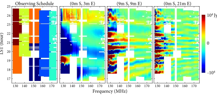
sessions, as shown in the left panel of Fig.3.

We first perform redundant calibration on the raw data,

using our redundant calibration pipeline described inZheng

et al. (2014), with further improvements described in

Ap-pendixA. Redundant calibration compresses the data in the

baseline direction from 2016 cross-correlation visibilities per snapshot to 112 unique baseline types, and automatically flags bad antennas, baselines, frequencies, and time stamps from the data. It is worth noting that redundant calibration

uses only the self-consistency between redundant baselines, and does not use any sky model. After redundant calibra-tion, we further compress the data to 0.75 MHz frequency bin width by averaging every 15 frequency bins. We then average over the time direction in 2 minute intervals. We empirically estimate noise during the time averaging step by performing linear fitting over 2 minutes of data and cal-culating the residual power.

At this stage, we have a data cube of 4 polarizations by 75 frequency bins by 240 time steps by 112 baselines. Since we have not used any sky information, the data is not yet absolute-calibrated, meaning that for each of the 4 × 75 = 300 different polarization-frequency data sets, we have 3 undetermined numbers: one overall amplitude, and two re-phasing degrees of freedom. These numbers cannot be determined without performing absolute calibration (as opposed to redundant calibration) with a sky model, which we describe in the next two sections.

4.1.1 Absolute Amplitude Calibration

The goal of absolute calibration is to determine three num-bers (an overall amplitude and two re-phasing degrees of freedom) for every time by baseline data set, where each data

set consists of more than 104 visibility measurements. This

is a drastically overdetermined system given a sky model. In this section, we discuss how we determine the overall ampli-tude. Since we intend to use the map obtained in this work to improve the GSM in a future work, we choose not to use the GSM as our sky model. Rather, we use Cyg A and Cas

A as our calibrators. After we obtain a map in Section4.2,

we will lock the amplitude of our map to the Parkes map at

150 MHZ (Landecker & Wielebinski 1970), so the amplitude

calibration and its error will only affect our spectral index results, not the amplitude of the map.

Our amplitude calibration is based on extrapolating the frequency-dependent secular decreasing flux models of

Cas A (Vinyaikin 2014) and the spectrum of Cyg A from

Vinya˘ikin(2006). Cyg A is an ultra-luminous, jet-powered, radio-loud galaxy. For our Cyg A calibration spectrum, we

use the model in Eq. 6a inVinya˘ikin(2006) of a transparent

source, with a power law spectrum with spectral index 𝛼,

observed through the absorbing ionized gas of our Galaxy. The data point used in the model at 152 MHz has a reported

3% error inParker(1968), and propagating the model

pa-rameters’ error bars leads to a maximum of 3.2% error in our frequency range.

The frequency dependence of the decreasing flux of Cas

A has been widely studied (seeHelmboldt & Kassim(2009)

and references, therein), and we adopt the empirical model inVinyaikin (2014) that fits to the accumulated published data taken from 1961 to 2011 from about 12 MHz - 93 GHz, including their most recent observations. The spectrum of Cas A is evaluated in frequency range 125-175 MHz, using

the fitted function in Eqs. 15 and 16 inVinyaikin (2014).

With this spectrum modeled at epoch 2015.5, and the model for the frequency dependent secular decrease in Eqs. 9 and

10 of Vinyaikin (2014), we evaluate the spectrum for Cas

A during MITEoR observations in August 2013, approxi-mately two years earlier. The largest source of error in the radio spectrum model of Cas A comes from our lack of com-plete understanding of the behavior of this supernova

(10)

rem-130 140 150 160 170 17 18 19 20 21 22 23 24 25

LST (hour)

Observing Schedule

130 140 150 160 170

Frequency (MHz)

(0m S, 3m E)

130 140 150 160 170 130 140 150 160 170

(9m S, 9m E)

(0m S, 21m E)

10

4

_Jy

-10

4

0

Figure 3. MITEoR’s observing schedule on the left and three sets of visibilities in the MITEoR data product on the right. Each of the six colors represent one of the nights between July 27th and August 2nd, 2013. Midnight corresponds to LST at roughly 21 hours. The real part of visibilities over time and frequency on three baselines of very different lengths are shown here. The white gaps in frequency and time are RFI events automatically flagged by the redundant calibration pipeline.

nant. In an evaluation of possible periodic deviations,

Helm-boldt & Kassim (2009) identify 4 possible modes ranging from 3 to 24 years, in a slightly lower frequency range of interest, 38 − 80 MHz, contributing to flux deviations from a secular decrease of up to 15%.

We calibrate in the LST range between 19 and 23 hours,

during which Cyg A’s elevation ranges from 59∘to 85∘, and

Cas A from 36∘ to 65∘. To minimize error introduced by

diffuse structures, we only include for calibration baselines longer than 8.6 wavelengths, which are the longest 9 base-lines at the lowest frequency and 34 at the highest frequency. After fitting using Cas A and Cyg A, we find about 15% residual on the visibilities. Since the errors introduced by the Galactic plane are averaged down over different baseline types, we estimate our amplitude calibration to go down by a factor equal to the square root of the number of baselines used. Thus, our absolute calibration has an overall error of about 5% at the lowest frequency and 2.5% at the highest frequency, relative to the calibrators.

4.1.2 Absolute Phase Calibration

As discussed inZheng et al.(2014), the two re-phasing

de-grees of freedom (or re-phasing degeneracies) in the visibility space correspond to shifting the beam-weighted sky image

𝑇_√𝑠(𝑞)𝐵(𝑞)

1−|𝑞|2 , and cannot be determined using only the self

con-sistency of visibility data without a sky model. However, this is only true for isolated snapshots in time. For instruments with large fields of view such as MITEoR, rotation of the sky does not exactly translate into shifting the beam-weighted sky image in the projected q-plane, so a constant shift of the beam-weighted sky image caused by constant re-phasing cannot be consistent with a rotating sky. Therefore, we can use a procedure conceptually similar to self-cal to determine the re-phasing: we first image using the visibility without

correcting for the re-phasing degrees of freedom, then use the image we obtain to solve for the re-phasing, and iterate until convergence. In theory, this can be done without any prior sky model, but since each iteration can be computationally expensive, we use the GSM to provide the initial re-phasing solution, and start iterating from there. It is worth noting that, at a given frequency and polarization, unlike self-cal which is solving for, say, 128 antenna calibration parameters at every time stamp, here we are only solving for 2 numbers for an entire observing session, so this iterative algorithm

has negligible impact on the validity of Eq. (12). For more

detailed discussions of redundant phase calibration, we refer

the readers toZheng et al. (2014) and AppendixA of this

work.

In addition, even for instruments whose array layout prevents making usable images, this “self-cal” approach can be applied to remove re-phasing degeneracies. Rather than

inserting regularization matrices to make A𝑡N−1A

invert-ible, if the goal is to calibrate out the re-phasing

degenera-cies, we can simply use a pseudo-inverse for A𝑡N−1A. For

example, for a redundant array with no short baselines, a pseudo-inverse will remove large scale structures in the im-age, but this has no effect when the resulting image is used as a model to simulate visibilities on those long baselines, so “self-cal” should work just as well.

4.1.3 Cross-talk Removal

We define cross-talk as additive offsets on visibilities that are proportional to the amplitude of auto-correlation, with a small but constant proportionality coefficient. In theory, the cross-talk terms can be solved for in an iterative fashion sim-ilar to how we determine the re-phasing degeneracies in the previous section. However, due to the level of thermal noise and systematics present in our data set, cross-talk on our

(11)

shortest baselines is highly degenerate with having a bright stripe in the trajectory of our local zenith. Thus for this work, we use the GSM to perform cross-talk removal. We use the GSM to simulate all the visibilities we measure, and for each visibility time series, we solve for the best fit using the GSM model visibility and the auto-correlation, and sub-tract the auto-correlation component from our data. Thus, for each visibility time series over a few hours, we use the GSM to fit and remove one degree of freedom corresponding to cross-talk.

4.2 Northern Sky Map Combining Multiple

MITEoR Frequencies

We apply the algorithm described in Section 2on the

MI-TEoR data to obtain our Northern sky map. We have shown

in Section3 that the MITEoR data can in principle make

high quality maps at individual frequency bins, but due to the systematics present in our data, which we discuss more in the next section, we are not able to make high quality maps using each individual frequency alone. Since in our frequency range the diffuse emission is dominantly synchrotron, which follows a smooth power law, we use techniques described in

Section2.5to combine multiple frequencies to form a single

map with an overall spectral index, as well as the beam-averaged spectral index as a function of time. We pixelize

the sky to HEALPIX 𝑛side = 64. Since the size of the

A-matrix is proportional to the number of frequency bins, and including the entire data set amkes the size of our A-matrix too large, we include only one out of every 5 frequency bins throughout the frequency range of 128.5 MHz to 174.5 MHz.

This forms an A-matrix of size roughly 6 × 105 by 4 × 104.

Since A has an order of magnitude more rows than columns,

computing A𝑡N−1A is the speed bottleneck and takes more

than 2 days when parallelized on a single CPU. In

compar-ison, inverting A𝑡N−1A takes about 3 hours.

In order to calculate the relative amplitude at different frequencies, to solve for the re-phasing degeneracies in the data, and to empirically estimate the level of noise and sys-tematics in each data set, we iterate the process described

in Section2.3until the amplitudes converge to within 0.1%

and re-phasings within 0.1∘

. At each iteration, we calculate visibilities using the solution from the previous iteration as a model, and for each frequency we fit for the re-phasing, the relative amplitude, as well as the overall error RMS. Both the best fit amplitude and the error RMS are used to re-weigh the noise covariance matrices for each frequency. When iterating, we prioritize the map’s accuracy in mod-eling visibilities over its noise properties, so we choose a

weaker regularization of 𝜖−1

= 1500 K. For the final map

we choose a stronger regularization with 𝜖−1

= 300 K to obtain lower noise in the map at a cost of lower resolution in the noisy areas. The map’s overall amplitude is locked to

the Parkes map at 150 MHz (Landecker & Wielebinski 1970)

using the overlapping region. Cyg A, Cas A, and their

“ring-ing” are removed using the CLEAN algorithm (H¨ogbom

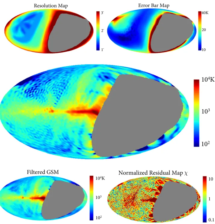
1974). The map we obtain together with its angular

reso-lution and error bars are shown in Fig.4.

4.3 Error Analysis

Fig.4shows that the map we obtain agree very well with

the prediction of the GSM at 150 MHz. In this section, we discuss the errors in our map and their possible causes in more detail. In terms of overall amplitude, the map’s overall amplitude is locked to the Parkes 150 MHz equatorial map (Landecker & Wielebinski 1970), which has 20 K uncertainty in zero level and 4% in temperature scale. In order to com-pare detailed structures in our result with the Parkes map

and the GSM, we calculate the normalized error 𝛿 maps,

shown in Fig. 4. The median 𝛿 compared to the filtered

GSM is 2.16, and 2.79 to the unfiltered Parkes map, which are slight higher than what one might expect.

There are a few factors that make the median𝛿 higher

than 1. Firstly, our modeling of our instrument is not per-fect, leading to error in our A-matrix. As we investigated

in detail inZheng et al.(2014), our beam model has up to

10% error in some directions. Our empirically estimated vis-ibility errors are dominated by slowly varying modes, and beam mis-modeling is the most likely cause. Another cause of error is the averaging over frequency, which assumes con-stant spectral index over the sky. As we show in much more detail in the next section, the spectral index changes by as much as 0.5 from the Galactic plane to out-of-plane regions, so this introduces an error for the edge frequencies on the

order of (175 MHz/150 MHz)0.5_{− 1 = 8%. Moreover, as we}

have seen in our simulation results in Fig. 1, pixelization

can also cause un-modeled error near high temperature re-gions such as the point sources (Cas A and Cyg A) and the Galactic center. Lastly, neither the GSM nor the Parkes map are the ground truth: the GSM at 150 MHz is essen-tially an interpolation product between a 45 MHz sky map and a 408 MHz sky map, with an estimated relative error

of 10% (de Oliveira-Costa et al. 2008). For the equatorial

Parkes map, due to its 2.2∘

resolution, we cannot apply the PSF matrix to it before comparing it to our result. The lack of PSF on the Parkes map leads to higher error in the

com-parison, which we think is what makes the median𝛿 higher

for the unfiltered Parkes map than for the GSM.

4.4 Spectral Index Results

4.4.1 Spectral Indices from 128 MHz to 175 MHz

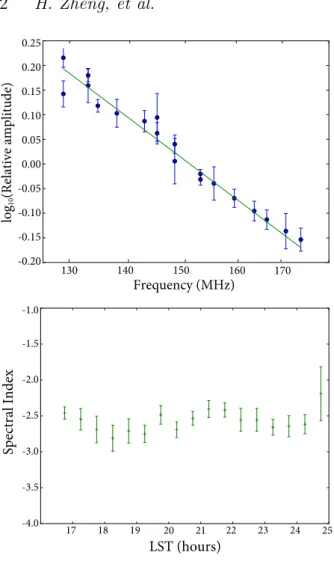
In the iterative process to compute the 150 MHz map, we also obtain relative amplitudes between all the data sets at different frequencies. At each frequency, we calculate visibil-ities using the 150 MHz map we obtained as a model, and compute the relative amplitude by comparing them to our data. We then perform a linear fit in the log(amplitude)-log(frequency) space, and compute an overall spectral index

of −2.73 ± 0.11, as shown in Fig. 5. The error bar is

calcu-lated using the residuals in the fitting process. In addition to this overall spectral index averaged over the entire data set, we also perform the same procedure on subsets of the data, and fit for spectral indices for every half an hour of LST. The resulting time series of spectral indices varies smoothly

between -2.4 and -2.8, as shown in Fig.5.

In comparison to our spectral index result, the

Exper-iment to Detect the Global EoR Signature (EDGES;

(12)

Resolution Map

3°

1°

2°

Error Bar Map

40K 10 20

10

4 _K

10

2

10

3 Filtered GSM

10

4

_K

10

2

10

3

10

4

_K

10

2

10

3

Dirty Map

10

0.1

1 Normalized Residual Map 𝜒

Figure 4. Top left: angular resolution map obtained from FWHM of the point spread functions. Top right: error bar map obtained from√Σ𝑖𝑖 based on empirically estimated noise covariance N. Mid: the northern sky map at 150 MHz, averaged from 128.5 MHz to

174.5 MHz, with Cas A and Cyg A removed using CLEAN. Bottom left: The GSM at 150 MHz, with the PSF matrix applied. Bottom right: 𝛿 as defined in Eq. (13), which represents the ratio between the difference between the maps and our map’s error bars. The median 𝛿 is 2.16.

(Rogers & Bowman 2008), centering at an out-of-plane

re-gion at declination −26.5∘and right ascension 2 h. Our

over-all spectral index agrees with the spectral index obtained by EDGES, with a 1.5𝜎 difference. However, the difference is likely not due to statistical variation alone. The overall spec-tral index we present is averaged over the northern sky, so we are observing a different patch of sky compared to EDGES. Unlike EDGES, our result is influenced by both Cyg A and

Cas A2_{. These strong radio sources have spectral indices}

of -2.7 and -2.8, respectively (Parker 1968;Vinya˘ikin 2006;

Vinyaikin 2014), so they would shift our results towards a steeper spectral index.

2 _{The point sources are present in our spectral index results}

be-cause our spectral index results are obtained in the visibility space, whereas the CLEAN algorithm that removed the point sources is performed in the image space.

(13)

0.25 0.20 0.15 0.10 0.05 0.00 -0.05 -0.10 -0.15 -0.20 160 170 130 140 150 Frequency (MHz) log 10 (Relative amplitude) 17 18 19 20 21 22 23 24 25 -4.0 -3.5 -3.0 -2.5 -2.0 -1.5 -1.0 Spectral Index LST (hours)

Figure 5. Map-averaged overall spectral index fit (top) and beam-averaged spectral index over LST (bottom). The relative amplitudes and error bars in the top plot are obtained from the iterative procedure described in Section4.4. For the bottom plot, each LST is observed on 5 different frequencies on 5 different nights (see Fig.3), so we can obtain a spectral index at each LST by fitting the overall amplitude over frequency with a power law. The error bars are 1𝜎, empirically estimated using the residuals of the power law fits.

4.4.2 Spectral Indices from 85 MHz to 408 MHz

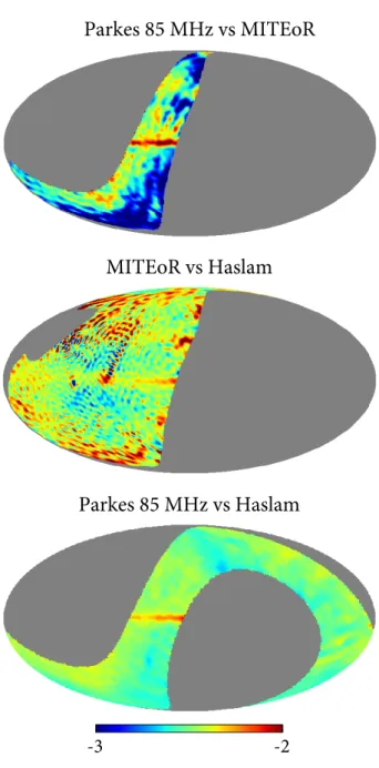
In addition to spectral indices in the EoR frequency range computed using the MITEoR data alone, we also calculate maps of spectral indices by comparing our MITEoR map to

the Parkes map at 85 MHz (Landecker & Wielebinski 1970)

and the Haslam map at 408 MHz (Haslam et al. 1981,1982;

Remazeilles et al. 2015). We compute per-pixel spectral in-dex maps for all three pairs of these three maps, as shown

in Fig.6.

The medians of the spectral indices shown in Fig.6are

−2.60 ± 0.29 ± 0.07, −2.43 ± 0.18 ± 0.04, and −2.50 ± 0.07, respectively. The first error bars come from the spread in spectral indices over the sky, and the second error bars come from 4% absolute calibration uncertainty of MITEoR. This is a very weak indication that the spectral index softens over the range from 85 MHz to 408 MHz. For comparison,

Platania et al.(2003) presented an overall spectral index of

−2.695 ± 0.120 between the 408 MHz (Haslam et al. 1981,

1982;Remazeilles et al. 2015), 1.4 GHz (Reich 1982;Reich

& Reich 1986;Reich et al. 2001), and 2.3 GHz (Jonas et al.

1998) maps, which also agrees well with an earlier study at

these frequencies inGiardino et al.(2002).

There are two spatial features worth noting in these maps. First, the Galactic plane has softer spectral indices than the out-of-plane regions. The median spectral indices

within 5∘of the Galactic plane for the three map pairs are

-2.27, -2.37, and -2.37, respectively. Softer spectral indices in the Galactic plane are also observed at higher frequencies in

Platania et al.(2003), whose spectral index map comes from three maps above the EoR frequency range, as mentioned above.

In addition to softer indices in the Galactic plane, there are regions that clearly deviate from the median near the Galactic poles, such as the blue regions in the Parkes vs MI-TEoR map, and the red regions in the MIMI-TEoR vs Haslam map. Since such departure is not seen in the Parkes vs Haslam map, this suggests that the MITEoR map is about 50 K lower in the Galactic pole regions than what the Parkes and Haslam maps jointly predict. There are two possible causes for this. The first is that the 50 K deficiency in the MITEoR map is due to systematic errors. However, the tem-peratures in these regions are about 240 K, so neither the 4% absolute calibration uncertainty nor the ∼ 15 K error bars can fully explain the 50 K difference. Another possible cause is that the MITEoR map has a higher dynamic range than the Haslam and Parkes maps, so that it recovers more de-tails at the low end of the temperature range compared to these maps. We leave a more careful investigation of this 50 K discrepancy to a future study.

5 SUMMARY AND OUTLOOK

We have presented a new method for mapping diffuse sky emission using interferometric data. We have demonstrated its effectiveness through simulations for both MITEoR and the MWAcore, where we obtained maps with better than

50 K noise and better than 2∘ resolution for both

instru-ments. We applied this method on the MITEoR data set collected in July 2013, which was absolutely calibrated us-ing Cyg A and Cas A. We obtained a northern sky map

averaged from 128 MHz to 175 MHz, with around 2∘

angu-lar resolution, 5% uncertainty in its overall amplitude, and better than 100 K noise. We also obtained an overall spectral index of −2.69 ± 0.11, and beam-averaged spectral indices that vary over LST between -2.4 and -2.8. Both the MITEoR visibility data and the 150 MHz sky map are available at

space.mit.edu/home/tegmark/omniscope.html.

As this is our first application of this new method, there are many aspects of it that we are excited to investigate in future work. Throughout this work, we have focused on reg-ularization matrices that are multiples of the identity ma-trix. However, since the sensitivity varies across the sky, es-pecially in the case of MWAcore, a regularization matrix whose strength varies with sensitivity may achieve a better balance between noise suppression and PSF. It is also inter-esting to study what the optimal array layout is for imaging

diffuse structure, along the lines ofDillon & Parsons(2016).

Since the Earth rotates in the East-West direction, we ex-pect the optimal array layout to be very different in the E-W direction than the N-S direction, perhaps similar to that of

(14)

Parkes 85 MHz vs MITEoR

MITEoR vs Haslam

Parkes 85 MHz vs Haslam

-3

-2

Figure 6. Spectral index maps between the Parkes map at 85 MHz, the MITEoR map at 150 MHz, and the Haslam map at 408 MHz. The MITEoR map is masked for regions with FWHM above 2.5∘or error bar above 20 K. The median spectral indices in these maps are −2.60, −2.43, and −2.50, respectively.

PAPER or CHIME (Shaw et al. 2014). Moreover, it is

in-teresting to investigate the effectiveness of this algorithm for instruments with much narrower primary beams, such as HERA. Lastly, it is valuable to perform further study in the effectiveness of this method for the purpose of cali-bration, such as calibrating the shorter baselines of MWA, which complements the existing calibration algorithms that focus on point source models for very long baselines.

Acknowledgments: MITEoR was supported by NSF grants AST-0908848, AST-1105835, and AST-1440343, the MIT Kavli Instrumentation Fund, the MIT undergradu-ate research opportunity (UROP) program, FPGA dona-tions from XILINX, and by generous support from Jonathan

Rothberg and an anonymous donor. AL acknowledges sup-port from the University of California Office of the President Multicampus Research Programs and Initiatives through award MR-15-328388, and from NASA through Hubble Fel-lowship grant HST-HF2-51363.001-A awarded by the Space Telescope Science Institute, which is operated by the As-sociation of Universities for Research in Astronomy, Inc., for NASA, under contract NAS5-26555. We wish to thank Jacqueline Hewitt and Aaron Parsons for helpful com-ments and suggestions, Evgenij Vinyajkin for his timely help with our error estimation for the Cyg A spectrum, Dan Werthimer and the CASPER group for developing and shar-ing their hardware and teachshar-ing us how to use it, Richard Armstrong, Matt Dexter, Alessio Magro, Mike Matejek, Qingxuan Pan, Robert Penna, Courtney Peterson, Meng Su, and Chris Williams for help with earlier stage of our hard-ware development and deployment.

REFERENCES

Ali Z. S., et al., 2015,ApJ,809, 61

Alvarez H., Aparici J., May J., Olmos F., 1997,A&AS,124, 315

Barry N., Hazelton B., Sullivan I., Morales M. F., Pober J. C., 2016, preprint, (arXiv:1603.00607)

Bowman J. D., Rogers A. E. E., Hewitt J. N., 2008,ApJ,676, 1

Dillon J. S., Parsons A. R., 2016, preprint (arXiv:1602.06259) Dillon J. S., et al., 2014,Phys. Rev. D,89, 023002

Dillon J. S., et al., 2015a,Phys. Rev. D,91, 023002

Dillon J. S., et al., 2015b,Phys. Rev. D,91, 123011

Furlanetto S. R., Oh S. P., Briggs F. H., 2006,Phys. Rep.,433, 181

Ghosh A., Koopmans L. V. E., Chapman E., Jeli´c V., 2015, MN-RAS,452, 1587

Giardino G., Banday A. J., G´orski K. M., Bennett K., Jonas J. L., Tauber J., 2002,A&A,387, 82

G´orski K. M., Hivon E., Banday A. J., Wandelt B. D., Hansen F. K., Reinecke M., Bartelmann M., 2005,ApJ,622, 759