HAL Id: hal-00868882
https://hal.archives-ouvertes.fr/hal-00868882
Submitted on 3 Jun 2021HAL is a multi-disciplinary open access
archive for the deposit and dissemination of sci-entific research documents, whether they are pub-lished or not. The documents may come from teaching and research institutions in France or abroad, or from public or private research centers.
L’archive ouverte pluridisciplinaire HAL, est destinée au dépôt et à la diffusion de documents scientifiques de niveau recherche, publiés ou non, émanant des établissements d’enseignement et de recherche français ou étrangers, des laboratoires publics ou privés.
Distributed under a Creative Commons Attribution| 4.0 International License
Automatic Differentiation of the Energy within
Self-consistent Tight-Binding Methods
Antonio Gamboa, Mathias Rapacioli, Fernand Spiegelman
To cite this version:
Antonio Gamboa, Mathias Rapacioli, Fernand Spiegelman. Automatic Differentiation of the Energy within Self-consistent Tight-Binding Methods. Journal of Chemical Theory and Computation, Amer-ican Chemical Society, 2013, 9 (9), pp.3900-3907. �10.1021/ct400214b�. �hal-00868882�
Automatic Differentiation of the Energy within Self-consistent
Tight-Binding Methods
Antonio Gamboa,* Mathias Rapacioli, and Fernand Spiegelman
Université de Toulouse, UPS, LCPQ (Laboratoire de Chimie et Physique Quantiques), IRSAMC, 118 Route de Narbonne, F-31062 Toulouse, France
CNRS, LCPQ (Laboratoire de Chimie et Physique Quantiques), IRSAMC, F-31062 Toulouse, France
1. INTRODUCTION
High-order response properties of molecular systems subjected to perturbations have received a growing interest in the past few years (for a recent review, see ref 1). For instance, the response to an electric field allows the description of nonlinear spectroscopy,2 through calculation of hyperpolarizabilities constants. Computing high-order energy derivatives with respect to geometric displacements can be used in optimization schemes or to build an analytical local potential energy surface (PES) with a Taylor expansion. Such a surface can then be used with approaches demanding fast energy computation to access quantum nuclear effects, like wave packet dynamics, quantum vibrational Monte Carlo, or calculation of infrared (IR) spectra including quantum effects with many-body mean-field or multiconfigurational methods for quantum vibrational pertur-bation theory.3−5
In the past decades, density functional theory (DFT) combined with the development of computational facilities has opened the route to the study of large systems. In many ab initio code using DFT, the third-order derivatives can be obtained as well as some partial fourth-order ones. In other calculations, harmonic constants may be derived with high level methods such as CCSD(T) and corrections with DFT third and fourth partial order derivatives are achieved to provide analytical surfaces.6
Tight-binding (TB) methods are much faster approaches that conserve the quantum description with explicit use of molecular orbitals (MO). Developed as the early quantum semiempirical methods (like the extended Hückel Hamilto-nians7), these approaches, which evolved to more complex formulations including for instance self-consistent processes, can be derived from ab initio methods (TB-HF from Hartee−
Fock8 or DFTB from DFT9−12). In all TB approaches, the solution of the electronic problem is achieved by the diagonalization (possibly iteratively) of the Hamiltonian matrix (eventually expressed in a nonorthogonal basis). The computa-tional efficiency of TB approaches relies on the use of a minimal atomic basis set and the fact that the Hamiltonian and overlap matrices elements are obtained from two-body parametrized functions or interpolated from precalculated points.
Among these TB approaches, density functional based tight-binding (DFTB9−12) is a computationally efficient DFT scheme in which all integrals are parametrized from DFT calculations. The second-order DFTB, also called self-consistent charge (SCC11) DFTB, is a refinement of this approach providing a more accurate description of moderately charged systems requiring a self-consistent diagonalization scheme. This approach has been widely used over the past decades to extract properties of systems for which DFT turns out to be too time-consuming in fields ranging from solid-state structures13to biomolecules.14
Analytical second-order SCC-DFTB energy derivatives with respect to geometry have been formulated by Witek et al.15and used to extract physical properties, in particular IR spectra in the harmonic approximation.16,17In this work, we describe how higher-order geometric derivatives of the energy can be computed analytically within the SCC-DFTB framework. The use of automatic differentiation enables a unique implementa-tion that allows the calculaimplementa-tion of these derivatives up to any ABSTRACT: We present and implement the calculation of analytical n-order geometric derivatives of the energy obtained within the framework of the density functional based tight binding approach. The use of automatic differentiation techniques allows a unique implementation for the calculation of derivatives up to any order providing that the computational facilities are sufficient. As first applications, the derivatives are used to build an analytical potential energy surface around the optimized geometry of acetylene. We also discuss the relevant anharmonic contributions that have to be considered when building such an analytical potential energy surface for acetylene, ethylene, ethane, benzene, and naphtalene.
order, provided that the CPU time and storage capabilities are sufficient.
Although the approach is applied here to SCC-DFTB, it is general for any self-consistent (or not) TB scheme. It can also be applied to achieve high-order derivations with respect to any perturbation (for instance electric or magnetic field) once the TB matrices elements derivatives with respect to this perturbation are known.
The paper is organized as follows. In the next section, after a brief presentation of the DFTB approach, we present the formalism allowing the calculation of any order properties derivatives within this framework as well as an analytic fit of DFTB parameters. We then benchmark the approach by comparing numerical and analytical calculation of derivatives. In the last section, the derivatives are used to build an analytical PES. We discuss the n-order derivative terms, that are quantitatively relevant on some examples.
2. METHOD
2.1. SCC-DFTB.In this section, we briefly review the basics of the SCC-DFTB method.9−12 It is derived from the Kohn− Sham (KS) DFT through an expansion of the DFT energy functional with respect to the electronic density around a reference density up to second-order. All three center integrals are neglected. With these approximations, the SCC-DFTB is given by
∑
∑
∑
ψ ψ γ = + ⟨ | ̂ | ⟩ + Δ Δ α β αβ α β αβ α β ‐ < E E n H q q 1 2 i i i i SCC DFTB atoms rep 0 , atoms (1)where Ĥ0is the KS operator at the reference density, n
iis the
electronic occupation of the KS MO Ψi, and Eαβrepis a repulsive potential between atoms α and β. The last term is the second-order contribution to the energy expressed through atomic pair
contributions involving a γ function of interatomic distances and atomic charges fluctuations Δqα.
The molecular orbitals are developed on a minimal atomic orbital (AO) basis set {ϕμ}
∑
ψ = ϕ μ μ μ c i i (2)leading to the matrix formulation
∑
∑ ∑
∑
γ = + + Δ Δ α β αβ μν μ ν μν αβ αβ α β ‐ < E E n c c H q q 1 2 i i i i SCC DFTB rep occ 0 (3)where H0and S are the KS and overlap matrices expressed in the AO basis. Atomic charge fluctuations are calculated with the Mulliken analysis approach Δqα = qα − qα0 where qα0 is the number of valence electrons in the neutral free atom and
∑ ∑ ∑
= α μ α ν μ ν μν ∈ q n c c S i i i iAs the atomic charge fluctuations depend on the MO coefficients, the energy minimization is performed through self-consistent cycles by solving the eigenvalue equation:
∑
−ε = ν ν μν μν c Hi ( iS ) 0 (4) with∑
γ γ = + = + + Δ μ α ν β μν μν μν μν ξ αξ ξβ ξ ∈ ∈ H H H H 1S q 2 ( ) , 0 1 0 (5)The matrix elements of H0, S, and E αβ
rep are interpolated from two-body DFT calculations.
Additional terms can be added to account for London dispersion (Edisp) forces as a sum over atomic pairs.18−20 In Figure 1.Hamiltonian and overlap matrix elements as functions of the distance for C−H interaction obtained from the analytical fit eq 6 and some of points obtained from the DFT integrals used to fit these parameters.
recent years, order terms with respect to the density have been introduced.21
2.2. Parameter Fitting. In the next section, n-order response properties resulting from a geometric perturbation ζ (geometrical change, electric field, etc.) will be derived analytically assuming the knowledge of the DFTB parameter derivatives with respect to this perturbation: ∂Hμν0/∂ζ, ∂Sμν/∂ζ, ∂Eαβrep/∂ζ, ∂γαβ/∂ζ.
DFTB matrices elements are computed at the DFT level for selected interatomic distances. Clearly, one cannot use low-order splines for high-low-order derivations and global analytic fitting of the DFTB parameters is relevant. The analytical fitting has been discussed by several authors either with Chebyshev polynomials22or standard polynomials.23One has to be aware of possible artifacts and transferability problems for very small matrices elements and out of the DFT tabulated ranges at long interatomic distances. Long-range artifacts can be in principle corrected via cutoff functions. The essential scope of the present paper is to present the analytical derivatives of the DFTB energy. This algebra is valid for any kind of derivable fitting functions. In the present work, we have expressed the interatomic elements of the Hamiltonian matrix at the reference density H0and the overlap matrix S as a polynomial function of the interatomic distance through a polynomial expansion:
∑
ϑ = =− R a R ( ) k n nk n 5 15 (6)The subindex k specifies the different types of interacting orbitals. For instance, in the case of second-row elements, the possible orbital interactions are s−s, s−p, p−s, (p−p)σ, and (p−p)π. As an example, we show in Figure 1 the results of the fitting process for the Hamiltonian and overlap matrices elements corresponding to s−s and s−p atomic basis orbitals for interaction of C−H atoms. We have used high-order polynomials in order to ensure the fit accuracy better than 9 × 10⁻⁵ Hartrees for all the DFT tabulated points. This is important to compute high-order derivatives. The n-derivatives of the H0 and S matrices are obtained by calculating the derivatives of the products of this function with the rotation matrices corresponding to various angular momenta.24The fact that the DFTB method only takes in account two-body interactions simplifies the calculations because all the derivatives that involve coordinates of three or more different atoms are zero.
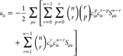
2.3. Analytical Derivatives. We first consider the calculation of n-order derivatives with respect to a single coordinate in the standard second-order SCC-DFTB. We follow here the approach of Masmoudi et al.25and extend it to the self-consistent scheme. In order to obtain the n-derivatives of the MO coefficients civ and the eigenvalues εi, we start
calculating the n-derivative of eq 4:
∑
− ε = ν ν μν μν c H S [ i( i )]n 0 (7)The superscript stands for the n-order derivative ∂n/∂ζn. We
suppose now that we have solved eq 7 for all orders k < n. So, in this equation, the only unknown terms are the highest-order ones ciνn and εin.
In order to calculate this terms, the derivatives of the coefficients ciνn are expressed as a linear combination of the MO
coefficients ciμ:
∑
= ν ν cin c u m m mi (8)Introducing this expansion in eq 7, using the formula of differentiation of a product
∑
= = −( )
AB n r A B ( )n r n r n r 0 (9)where nr( ) is the binomial coefficient n!/(r!(n − r)!) and multiplying by cjμcoefficients and summing over μ leads to the
following expression:
∑ ∑
ε −ε = − ε μν μ ν μν μν = − −( )
uji( i j) nr c c H( S ) r n j i r i n r 0 1 ( ) (10)If we extract the term corresponding to r = 0 from the sum and we apply again eq 9 to expand the product of (εiSμv)(n−r), we
can separate eq 10 in two cases. For i ≠ j, we have
∑
∑
∑ ∑
ε ε ε ε − = − + − μν μ ν μν μν μν μ ν μν μν = − = − − ⎜ ⎟ ⎛ ⎝ ⎜⎜ ⎛⎝ ⎞⎠ ⎞ ⎠ ⎟⎟( )
u c c H n k S n r c c H S ( ) ( ) ji i j j i n k n in k k r n j ir i n r 1 1 1 ( ) (11) and for i = j,∑
∑
∑ ∑
ε ε ε = − + − μν μ ν μν μν μν μ ν μν μν = − = − − ⎜ ⎟ ⎛ ⎝ ⎜⎜ ⎛⎝ ⎞⎠ ⎞ ⎠ ⎟⎟( )
c c H n k S n r c c H( S ) in i i n k n in k k r n i ir i n r 1 1 1 ( ) (12)where we are making use of the fact that ∑μνciμcjνSμν= δij.
These two sets of equations can be solved independently. For the non-SCC case, all the terms in the right-hand side (rhs) of eq 11 are known, as Hμv= Hμ0v. Therefore, this equation gives
the solution for each uiffor i ≠ j. On the other hand, in the SCC
scheme, the Hamiltonian matrix H depends on Δqn and
therefore on uif. The contribution of the n-order derivatives of
the Hamiltonian involving uifare identified and transferred to
the left-hand side (lhs) of the equation, leading to the linear system:
∑
A u = ′R c( < ,ε < ,H ≤ ,S ≤ )lm
ijlm lm k n k n 0k n k n
(13)
At first order, this system is known as the coupled perturbed equations (see, for instance,ref 26). The full expressions of Aijlm
and R′ are given in Appendix A. We notice that, although this system has to be solved for each order of the ciμderivatives, the
matrix Aijlm will allways remain the same and only a single
inversion of this matrix is necessary for the calculations of all derivatives.
To get the diagonal terms uii, we use the normalization
condition.
∑
= μν μ μν ν c S c ( i i )n1,...,nN 0 (14) that leads to∑ ∑ ∑
∑
= − + μ μ ν μν μ ν μν = − = − − = − − ⎜ ⎟ ⎡ ⎣ ⎢ ⎢ ⎛ ⎝ ⎞ ⎠ ⎤ ⎦ ⎥ ⎥( )
( )
u nr rp c c S n r c c S 1 2 ii v r n p r ipir p n r r n ir in r 0 1 0 1 1 (15)Once the MO coefficients are determined, eq 12 can be solved to obtain the eigenvalues derivatives εin.
In the general case, namely when we want to calculate a derivative according to more than a single coordinate, eq 7 is replaced by
∑
− ε = ν ν μν μν c H S [ i( i )]n1,...,nN 0 (16)where the general superscript n1, ..., nNstands for the following
derivatives: ζ ζ ∂ ∂ ∂ + + ... n n n Nn ... 1 N N 1 1 Equation 10 is replaced by
∑ ∑ ∑
∑
ε ε ε − = × − μν μ ν μν μν = − = − = − − − ⎛ ⎝ ⎜ ⎞ ⎠ ⎟ ⎛ ⎝ ⎜ ⎞ ⎠ ⎟ u n r n r c c H S ( ) ... ... ( ) ji i j r n r n r n N N j i r r i n r n r 0 1 0 1 0 1 1 1 ,..., ( ,..., ) N N N N N 1 1 2 2 1 1 1 (17)The procedure for solving the latter is exactly the same as the derivation according to a single variable. Besides, in the SCC case, the matrix Aijlm, that needs to be inverted to solve the
linear problem equivalent to eq 13, is exactly the same as the one for the case of derivation with respect to a single variable. This property is very favorable to save computational efforts.
Another fact that simplifies the calculation of the derivatives is the Wigner’s 2n + 1 rule,27 according to which, the knowledge of the n-derivative of the coefficients is sufficients to calculate the (2n + 1)-order derivative for the energy.
The applications in the next section section are carried on using second-order SCC-DFTB. Nevertheless, for sake of completeness, we show that analytical derivatives can also be carried on in the case of the third-order expansion of DFTB with respect to the density (DFTB3 approach21). The algebra of the derivatives is given in Appendix B.
3. BENCHMARKS
The algorithm presented in the previous section has been implemented in a preliminary version of the deMonNano28 code, a version of the deMon suite of programs devoted to large systems calculations with the DFTB approach. To benchmark the algorithm and its implementation, n-order derivatives have been calculated with the analytical approach presented previously and through finite differences. Both numerical and analytical derivatives calcuations have been performed with the analytical parameter fitting eq 6. The choice of the geometric displacement step, taken here as 0.01 bohr, results from a compromise between the fact that this value should be as small as possible to respect the differentiation definition but not too small to avoid numerical errors. We are calculating this derivatives in two steps. In the first one, we make an evaluation of the energy in a grid given by all the displacements: (±δx, ±2δx, ..., ±nδx), where n is the maximum order we want to calculate. The energy is then stored for all
points of this grid. In the second step, we use this stored values to calculate the derivatives. This way of calculating numerical derivatives makes it fast, but it has the drawback of requiring a very big amount of memory as we increase the size of the system.
As can be seen in Table 1, the relative error remains smaller than 0.1% up to third-order derivatives and increases up to 1−
7% for fourth-order derivative calculations. We also mentioned that the analytical differentiation is much faster than performing finite difference calculations as can be seen in Figure 2. This is
true, even when we are calculating the numerical derivatives with the efficient scheme previously described. Nevertheless, the numerical fourth-order derivatives for naphtalene were not calculated because the memory and time demands were too big. This fact indicates that, if we want to calculate derivatives up to fourth-order for big systems, one would need to do it without storing the values of the energy in a grid, and the time differences between analytical and numerical derivatives would be even larger than the ones showed in Figure 2.
4. APPLICATIONS
In this section, we present selected applications of n-order derivative calculations. We first present on a simple system (C2H2) how going up to fourth-order is mandatory to have a reasonably good description of the PES within a Taylor expansion. Finally, we discuss the distributions of derivative absolute values, depending on the number of involved normal modes for a variety of systems, namely acetylene, ethylene, ethane, benzene, and naphtalene.
Table 1. Maximum Relative Deviation between Numerical and Analytical n-Order (n = 2, 3, 4) Derivatives for Acetylene, Ethylene, Ethane, and Benzene Moleculesa
molecule second-order third-order fourth-order acetylene 9.8419 × 10⁻⁴ 1.0348 × 10⁻⁴ 6.8994 × 10⁻²
ethylene 1.0037 × 10⁻⁴ 9.3118 × 10⁻⁴ 1.1079 × 10⁻³
ethane 1.2842 × 10⁻⁴ 6.2790 × 10⁻⁴ 3.1483 × 10⁻²
benzene 1.9457 × 10⁻⁴ 6.8088 × 10⁻⁴ 1.2265 × 10⁻²
aAs the relative errors have no meaning for very small derivatives, we only considered derivatives that have an absolute value of at least 1% of the biggest derivative.
Figure 2. Time scale (seconds) comparison between calculation of analytical (dashed lines) and numerical (solid lines) as a function of the basis size (i.e., the dimension of DFTB matrices).
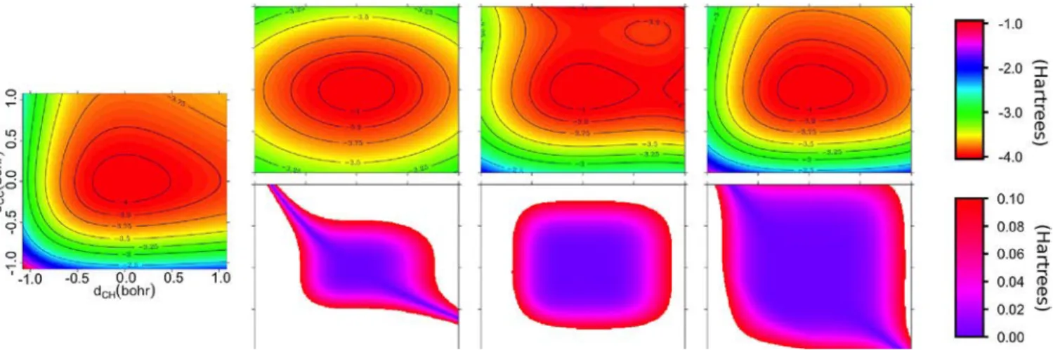
4.1. Building an Analytical Potential Energy Surface of Acetylene. As a first application of high-order derivative calculations, we focus on analytical PES reduced to two possible geometric deformations, namely the C−C and C−H bond length. Figure 3 present the corresponding potential energy subsurface, obtained either from single point DFTB calcu-lations either from Taylor expansion of the PES using n-order (n = 2−4) derivatives. The first plot shows that, around the minimum energy structure, iso-energetic contours look like a slightly deformed ellipse. Obviously, the harmonic approx-imation can not go beyond the ellipse shape description of the PES. This is not the case with the third-order expansion, the non-symmetric shape of the PES being recovered. However, two fictitious local metastable minima appear at intermediate distances from the most stable configuration. Such minima could have strong artificial effects for instance if some physical properties would be calculated by molecular dynamics on this approximated surface. Theses errors are washed by including fourth-order terms in the expansion, the local metastable minima being pushed much further from the most stable configuration.
4.2. Relevant Terms in n-Order Derivatives.Calculating high-order response properties in a DFT framework can be extremely computationally costly for systems even with a relatively small number of degrees of freedom. A solution often used is to calculate derivatives according to a selected number of modes. For instance, the calculation of fourth-order derivatives is often restricted to the dependence of one or two different normal modes Ni. Taking advantage of the
computational cost of DFTB and analytical high-order response implementation, it is possible to calculate all derivatives up to fourth-order for several molecular systems and to identify the significant terms. Figure 4 represents, for acetylene, ethylene, ethane, benzene, and naphtalene, the third- and fourth-order energy derivatives with respect to frequency scaled normal mode coordinates: Ñα= Nα(ωα)1/2, Nαbeing the normal mode resulting from the diagonalization of the mass weighted Hessian matrix.
For the third-order derivatives of the five studied systems, some derivatives with respect to two or three different normal modes are of the same order of magnitude (or even larger) as the ones with respect to one single normal mode.
Figure 3.PES of the acetylene molecule as function of C−C and C−H bond lengths obtained from single points calculations (left). In the upper panel, we show, from left to right, the PES obtained from Taylor’s expansion using analytical derivatives up to second-, third-, and fourth-order . In the lower panel, we plot the absolute value of the difference between the full PES and the n-order approximation.
Figure 4.Absolute values of third- and fourth-order derivatives of the energy with respect to frequency weighted modes coordinates, Ñα. The values of the derivatives are normalized with respect to the maximum value of the derivative in each case. Derivatives with respect to 1, 2, 3, and 4 different coordinates are separated by dashed lines.
For fourth-order derivatives, the situation is different between the three systems. In some systems, as acetylene and ethane, the derivatives according to one or two normal modes are the most important. However in the cases of ethylene, benzene, and naphtalene, derivatives with respect to 4 different coordinates are the same order of magnitude as the previous ones.
Such examples suggests that when only some values of derivatives are used to compute physical properties from a fitted surface, it is more consistent to calculate all derivatives and to use a threshold to eliminate some derivatives than to select it according to the number of involved normal modes. In a DFT framework, calculating all derivatives would have a computationally expensive cost. In such cases, DFTB could be used as a precalculation to select a limited number of derivatives to be calculated at the DFT level.
5. CONCLUSION
In this paper, we have derived general equation to calculate the
n-order response of the energy of a system with respect to a
geometric perturbation, calculated within SCC-DFTB ap-proach. The implementation of these equations in the deMonNano code makes use of automatic differentiation which enable the calculation of derivatives up to any order provided the fact that memory and computational time is available. Due to storage limitation, only derivatives up to fourth-order have been calculated in this work.
The implementation has been benchmarked by comparing the results with derivatives computed by the finite differences method. The analytical calculation is much faster than the latter approach. Such derivatives can be used to obtain an approximated PES of he system through a Taylor expansion up to a given order.
We notice that the equations reported in this paper are general and can be used to calculate the response with respect to any perturbation as long as the DFTB parameter derivatives with respect to this perturbation are known. This opens the route for instance to calculation of hyperpolarisabilities constants. The scope of this work was to express analytical n-order derivatives of DFTB properties to avoid its numerical calculations, without addressing the quality of DFTB PES. One should however keep in mind that DFTB is an approximated DFT scheme and that the quality of the n-order derivatives of any property relies on the DFTB accuracy itself, which can always be improved by refining parameters, introducing higher-order terms29or some specific corrections for instance to treat long-range dispersion and Coulombic interactions.18−20
As an illustration, we have discussed how including third- and fourth-order terms in the building of an analytical PES based on a Taylor expansion improves the local description of the acetylene PES. The role of high-order terms has been shown to have a significant effect. Finally, we have discussed the relative values of the derivatives for third- and fourth-order energy derivatives with respect to 1, ..., 4 normal mode deformations for acetylene, ethylene, ethane, benzene, and naphtalene. We showed that fourth-order derivatives involving two normal modes are for some systems less important than the same order derivatives involving 3 or 4 normal modes. As calculating derivatives with respect to all coordinates might be prohibitive at the DFT level and as the selection of the significant terms can hardly be done on the number of normal modes involved, we suggest that a fast DFTB high-order derivative calculation
could be performed in order to select the DFT derivatives to be calculated, when this level of description is required.
APPENDIX A: FULL EXPRESSION OF THE TERMS AIJLMAND R′ IN EQUATION 13
In this appendix, we give the steps to obtain eq 13 from eq 11 for the SCC case. The left part of eq 13 contains all the terms that involve ulmin eq 11. The hamiltonian Hμvis the sum of a
non-self-consistent part Hμ0v and the SCC component, Hμ1v
given by eq 5. The n-derivative of H1is given by
∑
∑ ∑
∑
∑
γ γ γ γ γ γ = + Δ = + Δ + + Δ μ ν μν ξ αξ ξβ ξ ξ μν ξ αξ ξβ ξ μν ξ αξ ξβ ξ = − ⎡ ⎣ ⎢ ⎢ ⎤ ⎦ ⎥ ⎥( )
H S q n r S q S q [ ] 1 2 ( ) 1 2 [ ( )] 1 2 ( ) n n r n r n r n , 1 1 (18) and∑ ∑ ∑
Δ ξ = ξ + + ω ξ χ ωχ ω χ χ ω ∈ qn gn n S (c c c c ) l l l ln l ln occ (19) where∑ ∑ ∑ ∑
∑
= + ξ ω ξ χ ωχ ω χ ωχ ω χ ∈ = − = − − ⎡ ⎣ ⎢ ⎢ ⎤ ⎦ ⎥ ⎥( )
( )
g n nr S c c S nr c c ( ) n l l r n r l l n r r n l r l n r occ 1 1 1 (20)The second term in the expression for Δqξn, is the only one in which appear the n-order derivatives of the coefficients ciμ, while
gξcontains only lower-order terms. The matrix Aijlmis obtained
after expressing the derivatives ciμn in terms of the coefficients uif
using eq 8 and grouping all these terms in the lhs of eq 11. The final expression is the following:
∑
∑
∑ ∑
ε ε δ δ γ γ = − − + × + μν μ ν μν ξ αξ ξβ ω ξ χ ωχ χ ω ω χ ∈ A c c S n S c c c c ( ) 1 2 ( ) ( ) ijlm l m il jm i j m l m l m (21)We notice that the expression of this matrix is equivalent to the one used to obtain the MO coefficient derivatives in the context of the DFTB-CI30
The rhs of eq 13 contains all the other terms and can be expressed as ε ′ < < ≤ ≤ = + + + + R c( k n, k n,H0k n,Sk n) Rij1 Rij2 Rij3 Rij4 (22) where
∑ ∑
ε = − μν μ ν μν μν = − −( )
Rij nr c c H( S ) r n j ir i n r 1 1 1 (23)∑
∑
ε = − μν μ ν μν = − −( )
R c c n r S ij j i r n in r r 2 1 1 (24)∑
∑ ∑
∑
γ γ = + Δ μν μ ν ξ μν ξ αξ ξβ ξ = −( )
R 1 c c nr S q 2 [ ( )] ij j i r n r n r 3 1 (25) and∑
∑
γ γ = + μν μ ν μν ξ αξ ξβ ξ R 1 c c S g 2 ( ) ij4 j i (26)APPENDIX B: FULL EXPRESSION OF THE TERMS AIJLMAND R′ IN THE DFTB3 SCHEME
In the third-order extension of the SCC-DFTB method, the Hamiltonian can be expressed as
∑
= + Δ μ α ν β μν ξ ξ ξμν ∈ ∈ H , H2nd q L (27)where Hμ2ndv is the second-order Hamiltonian given by equation
eq 5, and = Δ Γ + Δ Γ + Δ Γ + Γ ξμ αν β α αξ β βξ ξ ξα ξβ ∈ ∈ L 1 q q q 3( ) 6 ( ) (28) where γ Γ = ∂ ∂ ξα ξα ξ ξ q q0 (29)
Appling the same procedure used in the second-order case, we arrive to the correspondent expressions for the left and right parts in this extended scheme. For the matrix Aijlm, we have
∑
∑
∑ ∑
∑
∑ ∑
∑
∑ ∑
= − × + + + Δ Γ + + Δ Γ + μν μ ν μν ξ ξμν ξμν ω ξ χ ωχ χ ω ω χ ξ ξ αξ ω α χ ωχ χ ω ω χ ξ ξ βξ ω β χ ωχ χ ω ω χ ∈ ∈ ∈ ⎪ ⎪ ⎪ ⎪ ⎧ ⎨ ⎩ ⎫ ⎬ ⎭ A A c c S n L M S c c c c q S c c c c q S c c c c ( ) ( ) 3 ( ) 3 ( ) ijlm ijlm j i m l m l m l m l m l m l m 2nd (30)where Aijlm2ndis given for eq 21 and
= Δ Γ + Γ ξμν ξ ξα ξβ M q 6 ( ) (31)
The expression for the right part R′ is given by
ε ′ = + + + + + < < ≤ ≤ R c H S R T T T T T ( k n, k n, k n, k n) ij ij ij ij ij ij 0 2nd 1 2 3 4 5 (32)
where the second-order part is given by eq 22 and the rest of the terms are
∑ ∑
∑
= Δ μν μ ν ξ ξ ξμν = − −( )
Tij nr c c ( q L ) r n j i r n r 1 1 1 (33)∑
∑ ∑
= Δ μν μ ν ξ μν ξ ξμν = −( )
T c c n r S ( q L ) ij j i r n r n r 2 1 (34)∑
∑ ∑
= Δ μν μ ν ξ μν ξ ξμν = − −( )
Tij c cj i nr S q L r n r n r 3 1 1 (35) being∑
∑
= Δ μν μ ν ξ μν ξ ξμν Tij4 c cj i S q T4 (36) where∑
= Δ Γ + Δ Γ + Δ Γ + Γ ξμν α αξ β βξ ξ ξα ξβ = − − − − ⎛ ⎝ ⎜⎜ ⎞ ⎠ ⎟⎟( )
T n r q q q 3 3 6 ( ) r n r n r r n r r n r 4 0 1 (37) and∑
∑
= + Δ Γ + Γ + Δ Γ + Γ μν μ ν μν ξ ξ ξμν ξ ξα ξβ ξ α αξ β βξ ⎪ ⎪ ⎪ ⎪ ⎧ ⎨ ⎩ ⎛ ⎝ ⎜⎜ ⎞ ⎠ ⎟⎟ ⎫ ⎬ ⎭ T c c S g L q q g g 6 ( ) 3 ( ) ij j i n n n 5 (38) ASSOCIATED CONTENT Supporting InformationValues of the coefficients ankin eq 6. This material is available
free of charge via the Internet at http://pubs.acs.org/. AUTHOR INFORMATION
Corresponding Author
*E-mail: [email protected].
Notes
The authors declare no competing financial interest. ACKNOWLEDGMENTS
Computational support from the CALMIP/Toulouse facility is acknowledged as well as funding from ANR GASPARIM and CNRS/GDR2758.
REFERENCES
(1) Bast, R.; Ekstrom, U.; Gao, B.; Helgaker, T.; Ruud, K.; Thorvaldsen, A. J. Phys. Chem. Chem. Phys. 2011, 13, 2627−2651.
(2) Mukamel, S. Nonlinear Optical Spectroscopy; Oxford University Press: Oxford, U.K., 1995.
(3) Barone, V. J. Chem. Phys. 2005, 122, 014108. (4) Mills, I. M. Mol. Spectrosc. Mod. Res. 1972, 1, 115.
(5) Yagi, K.; Hirata, S.; Hirao, K. Phys. Chem. Chem. Phys. 2008, 10, 1781−1788.
(6) Carbonniere, P.; Pouchan, C. Theo. Chem. Acc. 2012, 131, 1−8. (7) Hückel, E. H. Z. Phys. 1931, 70, 204−86.
(8) Montagnon, L.; Spiegelman, F. J. Chem. Phys. 2007, 127, 084111−13.
(9) Porezag, D.; Frauenheim, T.; Köhler, T.; Seifert, G.; Kaschner, R.
Phys. Rev. B 1995, 51, 12947−12957.
(10) Seifert, G.; Porezag, D.; Frauenheim, T. Int. J. Quantum Chem. 1996, 58, 185−192.
(11) Elstner, M.; Porezag, D.; Jungnickel, G.; Elsner, J.; Haugk, M.; Frauenheim, T.; Suhai, S.; Seifert, G. Phys. Rev. B 1998, 58, 7260− 7268.
(12) Oliveira, A.; Seifert, G.; Heine, T.; duarte, H. J. Braz. Chem. Soc. 2009, 20, 1193−1205.
(13) Frauenheim, T.; Seifert, G.; Elstner, M.; Hajnal, Z.; Jungnickel, G.; Porezag, D.; Suhai, S.; Scholz, R. Phys. Stat. Solidi (b) 2000, 217, 41−62.
(14) Elstner, M. Theo. Chem. Acc. 2006, 116, 316−325.
(15) Witek, H. A.; Irle, S.; Morokuma, K. J. Chem. Phys. 2004, 121, 5163−5169.
(16) Witek, H. A.; Morokuma, K.; Stradomska, A. J. Chem. Phys. 2004, 121, 5171−5178.
(17) Witek, H. A.; Morokuma, K.; Stradomska, A. J. Theo. Comp.
Chem. 2005, 04, 639−655.
(18) Elstner, M.; Hobza, P.; Frauenheim, T.; Suhai, S.; Kaxiras, E. J.
Chem. Phys. 2001, 114, 5149−5155.
(19) Zhechkov, L.; Heine, T.; Patchovskii, S.; Seifert, G.; Duarte, H.
J. Chem. Theor. Comput. 2005, 1, 841−847.
(20) Rapacioli, M.; Spiegelman, F.; Talbi, D.; Mineva, T.; Goursot, A.; Heine, T.; Seifert, G. J. Chem. Phys. 2009, 130, 244304−10.
(21) Gaus, M.; Qiang, C.; Elstner, M. J. Chem. Theo. Comp. 2011, 7, 931−948.
(22) Frauenheim, T.; Weich, F.; Köhler, T.; Uhlmann, S.; Porezag, D.; Seifert, G. Phys. Rev. B 1995, 52, 11492−11501.
(23) Trani, F.; Barone, V. J. Chem. Theo. Comp. 2011, 7, 713−719. (24) Sherman, R. P.; Grinter, R. J. Mol. Struct.: Theochem 1986, 135, 127−133.
(25) Masmoudi, M.; Massat, C.; Poteau, R. Appl. Math. Comp. Sci. 1996, 6, 263−275.
(26) Wolff, S. Int. J. Quantum Chem. 2005, 104, 645−659. (27) Kristensen, K.; Jørgensen, P.; Thorvaldsen, A. J.; Trygve, H. J.
Chem. Phys. 2008, 129, 1−6.
(28) Heine, T.; Rapacioli, M.; Patchkovskii, S.; Frenzel, J.; Koster, A.; Calaminici, P.; Duarte, H. A.; Escalante, S.; Flores-Moreno, R.; Goursot, A.; Reveles, J.; Salahub, D.; Vela, A. deMon-Nano Experiment. http://physics.jacobs-university.de/theine/research/deMon/; ac-cessed 2013.
(29) Yang, Y.; Yu, H.; Uork, D.; Cui, Q.; Elstner, M. J. Phys. Chem. A 2007, 111, 10861−10873.
(30) Rapacioli, M.; Spiegelman, F.; Scemama, A.; Mirtschink, A. J.