Contents lists available atScienceDirect
Journal of Aerosol Science
journal homepage:www.elsevier.com/locate/jaerosciA model based two-stage classi
fier for airborne particles analyzed
with Computer Controlled Scanning Electron Microscopy
Mario Federico Meier
a,c,⁎, Thoralf Mildenberger
b, René Locher
b, Juanita Rausch
a,c,
Thomas Zünd
c, Christoph Neururer
a, Andreas Ruckstuhl
b, Bernard Grobéty
aaDepartment of Geosciences, University of Fribourg, Chemin du Musée 6, 1700 Fribourg, Switzerland
bInstitute for Data Analysis and Process Design (IDP), Zürich University of Applied Sciences (ZHAW), 8400 Winterthur, Switzerland cParticle Vision GmbH, c/o Fri Up, Annexe 2, Passage du Cardinal 11, 1700 Fribourg, Switzerland
A R T I C L E I N F O
Keywords: Particle classifier CCSEM/EDX Single particle analysis Cluster analysis Source apportionment
A B S T R A C T
Computer controlled scanning electron microscopy (CCSEM) is a widely-used method for single airborne particle analysis. It produces extensive chemical and morphological data sets, whose processing and interpretation can be very time consuming. We propose an automated two-stage particle classification procedure based on elemental compositions of individual particles. A rule-based classifier is applied in the first stage to form the main classes consisting of particles con-taining the same elements. Only elements with concentrations above a threshold of 5 wt% are considered. In the second stage, data of each main class are isometrically log-ratio transformed and then clustered into subclasses, using a robust, model-based method. Single particles which are too far away from any more densely populated region are excluded during training, pre-venting these particles from distorting the definition of the sufficiently populated subclasses. The classifier was trained with over 55,000 single particles from 83 samples of manifold environ-ments, resulting in 227 main classes and 465 subclasses in total. All these classes are checked manually by inspecting the ternary plot matrix of each main class. Regardless of the size of training data, some particles might belong to still undefined classes. Therefore, a classifier was chosen which can declare particles as unknown when they are too far away from all classes defined during training.
1. Introduction
Computer controlled scanning electron microscopy (CCSEM) is a powerful method for characterizing individual airborne parti-cles. It has the advantage that thousands of particles can be characterized individually in short time by localizing particles in backscattered electron images and measuring their composition with energy dispersive X-ray spectroscopy (EDS). Morphological parameters of individual particles can be obtained as additional characteristics of the particles. CCSEM as well as other methods for automated single particle analysis like Raman microscopy (Huang et al., 2013; Ivleva, McKeon, Niessner, & Poschl, 2007) or aerosol mass spectroscopy (Lanz et al., 2007; Richard et al., 2011) are particularly useful for apportionment studies of ambient aerosols. An important step of the apportionment procedure is the classification of the particles. Comparing ambient particle compositions with a library of reference emission particles allows assigning the particles to corresponding sources.
Many different approaches have been proposed for the classification process, including rule-based expert systems (e.g.Willis,
https://doi.org/10.1016/j.jaerosci.2018.05.012
Received 13 February 2018; Received in revised form 21 May 2018; Accepted 22 May 2018
⁎Corresponding author at: Department of Geosciences, University of Fribourg, Chemin du Musée 6, 1700 Fribourg, Switzerland.
E-mail address:[email protected](M.F. Meier).
Journal of Aerosol Science 123 (2018) 1–16
Available online 23 May 2018
0021-8502/ © 2018 The Authors. Published by Elsevier Ltd. This is an open access article under the CC BY license (http://creativecommons.org/licenses/BY/4.0/).
Blanchard, & Conner, 2002), hierarchical (e.g. Osán et al., 2001; Huang et al., 2013) and non-hierarchical cluster analysis (e.g. Bernard & Van Grieken, 1986), artificial neural networks (e.g. ART-2a) (Hopke, 2008) and other statistical approaches like principal component analysis (PCA) (e.g.Genga et al., 2012) and Partial Least Squares Discriminant Analysis (PLS-DA) (Tan, Malpica, Evans, Owega, & Fila, 2002).
Rule-based classifiers using chemical boundary conditions (CBC) are widely used and are suitable for simple situations with well-known sources (Ebert et al., 2002; Ebert, Weinbruch, Hoffmann, & Ortner, 2000; Ebert, Weinbruch, Hoffmann, & Ortner, 2004; Kandler et al., 2007; Kang, Hwang, Park, Kim, & Ro, 2008; Ro, Kim, & Van Grieken, 2004). For example,Lorenzo, Kaegi, Gehrig, and Grobéty (2006)studied particles originated from railway traffic by using a simple but efficient rule-based class building system, based on EDS net intensities of Fe, Si, Al, S and Ca.
Willis et al. (2002)proposed in the guidelines for the application of Scanning Electron Microscopy (SEM) of the US Environmental Protection Agency (U.S. EPA) a rule-based classifier, using chemical composition, morphological aspect ratio, total X-ray counts and grayscale brightness value.
Anaf, Horemans, Van Grieken, and De Wael (2012)compared their CBC classifier, based on procedures proposed byKandler et al. (2007), with a method for hierarchical clustering (HCL) (e.g.Osán et al., 2001). They concluded that CBC has advantages compared to HCL, as cutting the clustering dendrogram at different heights in the latter method is somewhat arbitrary. Furthermore, they pointed out that HCL has some difficulties with particles of mixed phases. These particles often have wide compositional ranges, which is difficult to map by hierarchical clustering. Nevertheless, HCL and non-hierarchical clustering are widely used for particle classification (Bein, Zhao, Wexler, & Johnston, 2005; Bernard & Van Grieken, 1986; Genga et al., 2012; Kim & Hopke, 1988; Moffet et al., 2013). Handling of outliers is a major problem in clustering. Most methods cannot properly deal with outliers, which have a strong impact on the cluster shapes.
In this paper, a new two-stage classifier for particles is presented. It consists of a combination of a rule-based first stage and a robust model-based second stage classifier. For each particle, element concentrations below 5 wt% are set to 0 wt% and the pro-portions of the remaining elements are rescaled to sum up to 100%. This elimination step is necessary because most spectra are noisy and, without thresholding, erroneous peak attributions are likely. For a system with better signal/noise ratio the threshold could be lowered. The set of the remaining elements defines the main class, which is subdivided in a second stage by a robust model-based clustering method. The resulting classes are hereafter called subclasses and are (after a transformation) described by (p-1)-dimen-sional ellipsoids with p being the number of elements present in the corresponding main class. Outliers are excluded automatically and hence have no effect on the shapes of the subclasses. Outliers found during classification are not assigned to any class and declared as unknown. As the classifier was trained with samples exposed to a broad range of sources, it is able to classify a broad range of airborne particles. If required, new classes can be easily included by further training. The classifier works for homogeneous particles, heterogeneous mixed particles and solid solutions.
2. Methods and materials 2.1. CCSEM
CCSEM for training and testing the classifier was performed with a FEI XL30 Sirion FEG Scanning Electron Microscope (SEM) equipped with an Energy Dispersive X-ray system (EDX, 10 mm2Lithium doped silicon detector by EDAX, with maximal energy
resolution of 128 eV) at the Department of Geosciences of the University of Fribourg, Switzerland. All samples were coated with a 40 nm thick carbon layer for better electrical conductivity. The analyses were performed with an acceleration voltage of 20 keV and spot size 4 (beam current = 10 nA). Data were acquired using the particle analysis module of the EDAX GENESIS software. Eighteen elements (Na, Mg, Al, Si, P, S, Cl, K, Ca, Ti, Cr, Mn, Fe, Ni, Cu, Zn, Ba and Pb) were used by default for classification. Lighter elements (C, N, O and F) were not taken into account for several reasons. As the sampling substrates (polycarbonatefilters and carbon stubs) and the coating consist of O and/or C, they interfere with the C and O content of the particles. Many of the particles consisting of light elements only were not recognized properly in backscatter images. This is due to poor contrast of these particles deposited on carbon based substrates. Net intensities have been corrected for background, matrix, absorption andfluorescence effects (ZAF-correction) before converting them into concentrations. ZAF-correction neglects geometric effects but assumes semi-infinite flat samples. The ZAF procedure is thus not ideal for particles that have an irregular surface or which are too small. Correction factors obtained by Monte Carlo simulations can provide more accurate results for the particle compositions (Armstrong, 1991; Choël, Deboudt, Osán, Flament, & Van Grieken, 2005; Ro, Osàn, & Van Grieken, 1999). Geometric corrections, however, are time consuming and test measurements on a standard glass sample described below show that the concentrations obtained from ZAF-procedure without geometric corrections for particles larger than 1.5 µm (geometric diameter) are precise and accurate enough for classification. In our setting, accuracy is less important than precision as long as measurement biases, i.e. systematic errors, are size independent. Changing the instrument or acquisition parameters may change bias of measurements. In this case all samples have to be reanalyzed by CCSEM and retrained. Further details on the SEM/EDS settings used during data acquisition are given inTable 1.
Total number of X-ray counts emitted from a given area of the substrate that is free of particles was used to check measurement set-up. For carbon based substrates (carbon pad, polycarbonatefilter etc.) and optimized measurement geometry the minimum was set to 6000 counts per second (CPS). This threshold and most settings described above are hardware specific and have to be adapted for other instrumental set-ups.
2.2. Preparation of standard sample
As the performance of the classifier depends on the precision and repeatability of measurements, tests on standard glass samples were performed. For that purpose the CRM glass standard no. 8 of the Society of Glass Technology (http://store.sgt.org/docs/ GLASS8.pdf) was used. The chemical composition of the glass as indicated by the provider is given inTable 2. Glass fragments were milled for 30 s in a high energy mill (SPEX8000M). A small amount of the resulting powder was given into a beaker, which was closed with a plastic paraffin film (Parafilm). The particles were brought into suspension by shaking the beaker. Then the Parafilm was removed and the beaker was turned upside down. The bigger particles and agglomerates were allowed to sediment during 30 s. Finally, a polycarbonate membranefilter (typical filters used for active particle sampling) mounted on a SEM aluminum stub was positioned under the beaker to collect a part of the still suspended small particles. These“standard” samples with particles in a size range of 0.1–100 µm geometric diameter were carbon coated prior to analysis by CCSEM.
2.3. Ambient particle sampling
Environmental samples for training and classifying were taken during different air quality studies with two different sampling methods. Most of the samples were taken using a Sigma-2 sampler. This sedimentation-based passive sampler is certified for quantitative sampling of particles with a geometric equivalent diameter between 2.5 and 100 µm (VDI, 2013). The particles were sampled directly on sticky carbon pads (12 mm diameter, Plano Spectro Tabs), which are suitable for SEM analysis.
Particles were also sampled actively on polycarbonate membranefilters (pore size: 0.4 µm, Nuclepore). The air flow was kept at 4 l min−1. Thefilters were mounted in a housing, which was developed by the Swiss Federal Laboratories for Materials Science and Technology (EMPA) and slightly modified by the University of Fribourg (Lorenzo, 2007).
Samples were taken at manifold sites, including urban sites (e.g. Mexico City, Zürich), natural background sites (e.g. Swiss Alps), and sites close to different anthropogenic or natural particle sources (highways, railways, construction sites, quarries, landfills, industries, active volcanoes etc.). In total, over 55′000 single particles from 83 samples were analyzed.
Table 1
Instrumental settings used for CCSEM.
Instrumental settings
Microscope parameters
Microscope FEI XL30 Sirion FEG
EDS-detector Lithium doped silicon detector by EDAX (10 mm2with maximal energy resolution of 128 eV)
Acceleration voltage 20 keV
Spot size / Beam current 4 / 10 nA
Magnification (image size) ≥ 1000 × for particle 2.5 − 80 µm; image size: 120 × 92 µm ≥ 2000 × for particle 1.5 − 40 µm; image size: 60 × 46 µm EDS parameters
EDS software EDAX GENESIS
Image resolution for image analysis 2048 × 1600 pixels
Acquisition time 15 s
Elements and used emission lines (in parentheses) for quantification
Na (K), Mg (K), Al (K), Si (K), P (K), S (K), Cl (K), K (K), Ca (K), Ti (K), Cr (K), Mn (K), Fe (K), Ni (K), Cu (K), Zn (K), Ba (L) and Pb (M)
Area of projected particle surface included into EDS-analysis (Lorenzo et al., 2007)
80%
Peak recognition criteria 1.5 × background
Table 2
Chemical compositions of CRM glass standard no. 8 of the Society of Glass Technology measured by wet chemical methods and elemental com-position excluding oxygen renormalized to 100%.
oxide oxide wt% standard deviation element element wt%
B2O3 0.36 0.03 B 0.17 Na2O 0.23 0.012 Na 0.26 MgO < 0.02 – Mg < 0.02 Al2O3 0.05 0.008 Al 0.04 SiO2 56.34 0.054 Si 39.58 K2O 11.85 0.13 K 14.78 CaO < 0.02 – Ca < 0.02 TiO2 0.02 – Ti 0.02 Fe2O3 0.01 0.0004 Fe 0.01 As2O3 0.32 0.026 As 0.36 PbO 30.59 0.101 Pb 44.74 Loss at 550 °C 0.21 – – –
3. Particle classifier 3.1. Outline
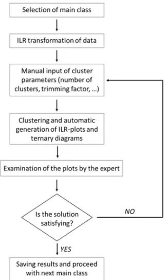
The classifier described here is designed to automatically attribute any particle in ambient air to a specific class, including the class“unknown”. To reach this goal, the classifier first needed to be trained with abundant data that have been labeled (classified) before by some other procedures. This process is often time consuming and expensive as in general data have to be labeled manually. In our case, the training set was so large that labeling had to be automated as much as possible. Thus, particles are clustered into classes, which were checked visually by experts. Their feed-back was then used in an iterative process to adapt the clustering parameters to produce chemically consistent classes.
Even though the training set consisted of more than 55,000 particles, the resulting classes do not cover the broad spectrum of all possible airborne particles. Ambient air is an open system, where new kinds of particles can appear at any time. Hence, the identified set of classes must include a special class called“unknown”, which contains all particles whose elemental compositions are too far away from any of the identified classes. This restricts the potential clustering methods to model-based ones. The classifier described here computes the distances of the particle to all identified classes. The particle is then assigned to the nearest class unless this distance is larger than a given threshold value. In the latter case, the particle is labeled as“unknown”. We use a simple Gaussian model for the classes, where all particles (after a suitable transformation) are described by a (p-1)-dimensional normal distribution with p being the number of used elements. The corresponding mean vector and covariance ellipsoid indicate center, shape and spread of the cluster. For a general introduction to model-based clustering see e.g.Everitt, Landau, Leese, and Stahl (2011). For all statistical calculations, the open-source statistical package R was used (R Core Team, 2018).
3.2. Training: Constructing particle classes by clustering
Training the classifier and classifying particles are two-stage processes. First, a simple rule-based method divides the particles into classes of particles consisting of the same elements. These are called main classes hereafter. As this stage is rule-based, it does not need any training. In a second stage (training step), a robust model-based clustering method is applied separately for each main class consisting of more than one element. The clusters within the main classes are called subclasses hereafter.
3.2.1. First stage: Main classes
In our application, the composition of a particle is based on weight proportions of the 18 elements mentioned inSection 2.1. Mathematically, we treat a particle as an 18-dimensional vector whose components are non-negative (but may be zero) and sum to 1 (or 100%). Due to the constant-sum-constraint, the vectors are (affine-)linearly dependent and the corresponding points lie in an (affine) subspace of dimension 17.
Quantifying elemental proportions with CCSEM involves a certain inaccuracy. Particularly, low signal intensities and/or im-precise background subtractions may lead to a spurious elemental composition. The detection limit is a function of the used equipment (hard- and software), the analytical settings, matrix effects and the measured elements. We applied a conservative peak detection limit of 1.5 times of the background and introduced a relatively high detection limit of 5 wt% to safely get rid of spurious compositions. For each particle, concentrations for elements below 5 wt% are set to 0 wt% and the proportions of the remaining elements are rescaled to sum up to 100 wt%. As a consequence of the high detection limit, the number of elements in a particle may be smaller than the true number of elements. This procedure attributes to each particle a set of elements whose proportions are ≥ 5 wt%, defining the main class the particle belongs to. By eliminating elements with proportions below 5 wt%, the dimensionality is reduced and hence the clustering problem is simplified (seeSection 3.2.2). Main classes with less than 10 particles were considered as statistically unsupported for clustering and were hence excluded from training.
Three cases illustrate the procedure. A quartz (SiO2) particle belongs to the main class“Si”, since oxygen is not taken into account
and only the proportion of the element Si is≥ 5 wt%. A homogeneous sea salt particle (NaCl) belongs to the main class “Na-Cl”, as the proportions of Na and Cl are both≥ 5 wt%. If this particle would additionally contain K with a proportion ≥ 5 wt%, it would belong to the“Na-K-Cl” main class. However, if the K proportion would be < 5 wt%, the particle remains in the “Na-Cl” main class. As the element list consists of 18 elements, a main class with all 18 elements is theoretically possible. However, no particles with more than seven elements with proportions≥ 5 wt% after rescaling were found.
3.2.2. Second stage: Subclasses
In the second stage, the particles within each main class with more than one element are clustered into subclasses. The choice of the clustering method - and the method for classifying new particles as described in subsection 3.3 - has to be adapted to the nature of the data. Our data are compositional (Aitchison, 1986; Van den Boogaart & Tolosana-Delgado, 2013). The sum of all components is always 100%. This means that the components will both be linearly dependent and non-negative, leading to severe problems when standard methods are applied without any transformation. For all particles in a main class, all elements except the ones defining the main class are dropped before further data processing. Hence, a particle in a subclass defined by p elements with proportions ≥ 5 wt % (e.g. p = 3 for the Si-Al-K class), is represented by a p-dimensional vector. The components, which are now strictly positive, are rescaled to sum up to 100% (or 1), and are therefore again linearly dependent. The vectors are transformed through an Isometric Log-Ratio transformation (ILR transformation) (Egozcue, Pawlowsky-Glahn, Mateu-Figueras, & Barceló-Vidal, 2003) to an p-1 dimen-sional subspace as implemented in the compositions package for R (Van den Boogaart, Tolosana, & Bren, 2014). The resulting
components are linearly independent. The effects of transformation are shown inFig. 1. This non-linear transformation belongs to a family of transformations based on the logarithm of ratios of proportions. These are essentially the only ones that simultaneously satisfy a number of invariance properties, and among these the ILR transformation has the advantage of avoiding degenerate cov-ariance matrices (Egozcue et al., 2003;Van den Boogaart and Tolsana-Delgado, 2013) which is essential for applying the chosen clustering method. By applying the ILR transformation separately within each main class, its major limitation is avoided: its inability to cope with zero components. The resulting vectors are not constrained to lie in a special subset of the space, so that all clustering and classification methods developed for general (non-compositional) multivariate data can be applied to the transformed points. Furthermore, clusters of compositions often tend to look approximately Gaussian after ILR transformation, which is a requirement for the cluster algorithm used here.
After the ILR-transformation, data were clustered using the Robust Trimmed Clustering method (Garcia-Escudero, Gordaliza, Matran, & Mayo-Iscar, 2008), which is implemented in the R package tclust (Fritz, Garcia-Escudero, & Mayo-Iscar, 2012). In tclust, data are modeled as a mixture of multivariate Gaussian distributions parametrized by their means and covariance matrices, leading to a segmentation of the data points into ellipsoid-shaped clusters. The ellipsoids are allowed to have different sizes, shapes and orientations, although some constraints have to be enforced in order to exclude undesired extreme solutions. In our case, we have set a constraint on the ratio of the largest to the smallest eigenvalue across the covariance matrices of all subclasses within a specific main class
Tclust robustly estimates the centers, spread and shapes of the clusters, allowing for a fraction of the data points not to be assigned to any of the clusters. This prevents outliers from influencing the shape of clusters formed from “good” data points (Fig. 2).
In cluster analysis, outliers are not necessarily points that are remote from the majority of points but can also be points that lie between clusters (sometimes called“bridge points”). Small patches of particles that potentially form a subclass of their own are considered to be outliers if the particles are so few that size and shape of the cluster cannot be reliably estimated. In that case, we do not want these to be included into another larger cluster. The proportion of points not used infitting the clusters has to be specified by the user and is also called the trimming fraction (denoted byα) and can take values between zero and one. Although the proportion is set by the user beforehand, the points that are regarded as outliers are determined by the algorithm. The obtained clusters correspond to Gaussian distributions with different mean vectors and covariance matrices. These are later used for classification. The following combination of settings for the algorithm worked fairly well for the majority of main classes in our training data. Trimming fractionα was set to 0.05. The upper limit for the ratio between the largest and smallest eigenvalue across the covariance matrices of all clusters within a specific main class was set to 3. We allowed for these parameters to be changed if this lead to a more meaningful grouping, but it was applied rarely. The exceptions belong to main classes with poorly populated subclasses. For 37 out of 227 main classes, the trimming fractionα was set to smaller values between 0.001 and 0.02 (instead of 0.05). The ratio γ of the largest to the smallest eigenvalue was constrained to 1 (instead of 3) in two main classes, enforcing circular rather than ellipsoid-shaped clusters. The only parameter always to be chosen manually by a domain expert was the maximum number of clusters that was searched for. There are methods to do this automatically but the results were not satisfactory. How to choose the number of clusters is described inSection 3.2.3.
Fig. 1. ILR-Transformation of compositional data. Compositional data of three elements (A, B and C) lie along six different lines in a ternary diagram (left). The same data after ILR transformation plot in a two-dimensional subspace (right). Points where at least one of the three considered elements is below 5% are plotted in light grey. All compositions with the same ratio between two elements are arranged along a straight line after ILR transformation (orange, red and brown lines). All compositions arranged along a straight line in the ternary diagram without a constant ratio between two elements are arranged along a curved line after ILR transformation (blue, purple and green lines).
3.2.3. Deciding on number and shape of clusters
The number of clusters and therefore of subclasses within a main class was determined manually as follows (seeFig. 3): First, binary (p = 2) and ternary (p≥ 3) diagrams of the main classes were automatically generated by the classifier. For main classes with p > 3, sets of diagrams with two corners representing single elements and the third corner representing the sum of the remaining elements were generated (seeFig. 4). These ternary diagrams were inspected together with the corresponding plots of the ILR transformed data points in order to estimate a rough number k of clusters (subclasses). The ILR plots are important as it can be argued that this is the correct geometry to analyze compositional data, and assuming ellipsoid-shaped clusters makes only sense in the transformed space. Since the transformation is non-linear, distances and geometrical shapes are not preserved: Equidistant points in the ternary diagram transform into points of the ILR space, whose distance to each other become the larger, the closer the points lie to the border in the corresponding ternary diagram (compare points in light grey with points in dark grey inFig. 1). Therefore, the pattern of the points in the ILR-transformed space looks different, especially for points near the border of the ternary diagram. However, this effect becomes of minor importance (area in dark grey) due to the ≥ 5 wt% criteria in the first classifying stage. The ternary plots are also crucially important since they are easier to interpret in terms of geochemistry, because chemical compositions can be obtained directly from ternary diagrams. The graphically determined number of subclasses and the default values forα = 0.05 andγ = 3 were used as input for the automatic clustering procedure. The particles were then classified (seeSection 3.3) and dis-played in ternary diagrams and ILR space, where each subclass was plotted in a different color. Additionally, elemental compositions of well-known substances such as mineral phases, metallic alloys or other known compositions of more complex substances (e.g. tire wear) were displayed in the plots and their position relative to the classified particles were checked. When the shape of any of the subclasses did not satisfy, the number of subclasses was increased or decreased. If the results were still not satisfactory, nonstandard values forα and γ were tried. The optimum parameters were then chosen among these alternatives. This approach worked well especially for homogenous phases. All ternary plots containing color-coded subclasses and elemental compositions of well-known substances are given in theSupplementaryfile 1.
In ternary diagrams the compositions of phases and phase mixtures cover an area with certain shapes. Individual phases with constant composition plot ideally in one point. Phases with varying compositions (solid solutions) and mixed phases (particles composed of two or more phases) plot in an extended area. The shape of the area can give some indications of the number of phases present in mixed particles or the number of varying elements in a solid solution. When the compositions of the phases in terms of the components defined in the corner of a ternary diagram are linearly independent, mixtures rich in one of the phases will lie close to the composition of that phase. For example, mixed particles consisting of quartz (SiO2) and halite (NaCl) lie in a ternary Na-Cl-Si diagram
along the mixing line ranging from a halite dominated to a quartz dominated mixture. It had to be decided whether this should be one cluster, representing all quartz-halite-mixtures, two clusters representing a quartz dominated and a halite dominated cluster or more than two clusters. The solution chosen for this particular case has three clusters: A halite dominated cluster, a quartz dominated Fig. 2. Showcase for different procedures to estimate a cluster ellipsoid in the two- dimensional space. ILR transformed data points can be clustered in different ways. The dashed red ellipsoid is based on standard (non-robust) estimation of all points in the plot. Please note the outlier colored in red at bottom right: the latter is the reason for the increase of one of the axes of the red ellipsoid, relative to the stippled blue ellipsoid, which is also based on standard, non-robust estimation of all points except the red one. The long axis of the blue ellipsoid is strongly influenced by the blue point at the left. The green ellipsoid is based on a robust estimation of all points, including all outliers. Nevertheless, this ellipsoid is a reliablefit. Robust estimation is crucial for proper estimation of ellipsoids, when a) larger measurement errors have to be taken into account, b) ellipsoids have more than 2 dimensions and / or c) they have to be estimated without graphical inspection of data.
cluster and one cluster in between (Fig. 4). Some“unknown” particles (black circles) are far from the quartz-halite mixing line and hence are particles that definitively do not belong to the Na-Cl-Si-mixture. But some others are on this line, between the green and the yellow clusters. The classification of these particles as “unknown” has geometric reasons as the stripe in which the particles lie in the log transformed space is in our case modeled by three ellipses, which of course do not cover homogeneously the complete area of the stripe.
Particles belonging to a simple solid solution with endmembers and intermediate members with compositions AxB1-xC (with A, B
= elements and C = element or sum of Elements), are classified into the three different main classes ABC, AC and BC, depending on the proportion of A and B. When the proportion of A or B is below 5 wt%, the main class is BC or AC, respectively.
In a ternary plot representing the compositions AC and BC, the solid solutions AxB1-xC, lie along a mixing line, which cannot be
distinguished from mixed particles consisting of two phases. Solid solution phases are, therefore, clustered the same way as mixed particles. InSection 4.2alkali feldspars are discussed to illustrate this situation on the basis of a concrete example.
The selection of numbers of clusters becomes more complicated the more elements the main class consists of, as more dimensions have to be considered. For main classes with p > 3 elements, a ternary plot matrix is constructed that shows all possible ternary diagrams with two variables representing individual elements and the third representing the sum of all remaining elements.Fig. 5 shows all particles of the training set belonging to the main class Si-Ca-Na-Cl. Each ternary diagram shows the same particles from another perspective. The main class Si-Ca-Na-Cl essentially consists of mixed particles composed of calcite (Cc, CaCO3,), quartz (Qtz,
SiO2) and halite (Hl, NaCl) in different proportions. For most of the ternary diagrams in the 4 × 4 matrix, the mixed particle
compositions are within a triangular shaped area. The corners of these triangles correspond to calcite-rich, quartz-rich and halite-rich mixed Cc-Qtz-Hl particles. In the ternary diagrams, calcite and quartz correspond to the Ca- and Si-corners, respectively, while halite either to the Na- or the Cl- or a point half-way between the Na- and Cl-corners. In ternary diagrams in which Si and Ca proportions are summed up, data points representing Cc and Qtz overlap. The representation of Cc-Qtz-Hl particles is degenerated, collapsing to a binary mixing line with the endmembers halite and all possible calcite/quartz mixtures, respectively. Four distinct subclasses were found, coded by distinct colors inFigs. 5 and 6.
Fig. 3. Scheme defining number and shape of clusters within a main class.
Actually, the particles have been clustered in the ILR transformed three-dimensional space as illustrated inFig. 6by the plot matrix. The four clusters separate quite well in the projection of ILR component 1 and 2 and 1 and 3, respectively. Nevertheless, a complete separation need not be visible in a plot matrix as a (p-1)-dimensional distribution is projected into a 2-dimensional sub-space. The higher the dimension of the original space, the lower is the probability that the subclasses can be observed as well separated clusters in the 2-dimensional subspace. Another technique of visualization of clusters of particles in a high dimensional space is the biplot, shown in theSupplementaryfile 2.
3.3. Classification of new particles
Classifying, i.e. assigning new particles to the previously defined classes, is done analogously to clustering. First, new observations are thresholded, renormalized and assigned to main classes. The same ILR transformation, which was used for this main class during training, is then applied. Thus, the new particles are mapped to the same p-1-dimensional space as all previously classified particles of the same main class. Classification then consists of assigning a particle to the closest subclass within the main class, or deciding that the new particle is too remote from all existing subclasses to belong to any of them. The distance to a subclass is measured by the Mahalanobis distance to the subclass center. The Mahalanobis distance assumes that the data point distribution in the subclasses is approximately Gaussian and takes into account the shape and orientation of the covariance matrix. This allows for meaningful comparisons of distances even when the covariance matrices are very different and the spread of the subclasses is not isotropic. The squared Mahalanobis distance of a new point x to be classified to the mean μiof the i-th subclass is given by
= − − −
d x μ( , i) (x μi)TΣ (x μ)
i i
2 1
whereμiis the mean vector andΣi−1is the inverse of the covariance matrix of the Gaussian distribution of the i-th subclass. It is
known (e.g. see example 3.4.2 of the work byTimm, 2002) that for a point randomly generated from a non-degenerate Gaussian distribution with mean vectorμiand covariance matrixΣi, the squared Mahalanobis distance toμiis a random variable with a
Chi-Square distribution with degrees of freedom equal to the dimension (in our case (p-1) for a main class defined by p elements). Even in cases where the normal distribution isfitted to the data (as is the case here) the chi-square distribution is still a good approximation. We now compute the Mahalanobis distances of the new observation to all subclass means and assign it to the closest subclass. If the squared distances to all subclass means are larger than the (1-β) quantile of the chi-square distribution with (n-1) degrees of freedom, we conclude that the observation does not belong to any of the previously defined subclasses. We use β = 0.01, leading to the 99% quantile. When a new data point has a squared Mahalanobis distance to a subclass center that is larger than the 99% quantile, the point is farther away from the center than 99% of the points randomly drawn from the normal distribution induced by the cluster. If this is valid for all subclasses, the point is labeled as“unknown”.
Note that when running the classification algorithm on the training set, even for α = β, the points not classified are not ne-cessarily the points trimmed as outliers during clustering. Clustering considers all particles simultaneously while classification identifies particles based on distances to individual subclasses. The sets should be very similar, though. In the case of only one cluster Fig. 4. Ternary diagram (left) and ILR-plot (right) of the Si-Na-Cl main class with a NaCl dominated subclass (red), a SiO2dominated subclass (green) and a subclass in between. Due to the≥ 5 wt% criteria of the first classifying stage, the red subclass ends at 5 wt% Si. Mixed particles with less than 5 wt% Si belong to the Na-Cl main class. Black circles are particles which do not belong to any cluster and are classified as “unknown” within the main class (for further discussion of“unknown” particles see main text inSection 3.2.3). Black crosses correspond to the centers of the clusters.
for a main class, some observations may not be assigned to the cluster as they are judged to be too far from its center.
4. Results
4.1. Standard glass sample
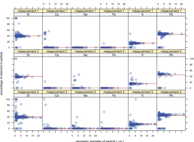
As mentioned inSection 2.2the powder of a standard glass sample was used for testing the analytical settings and the perfor-mance of the classifier with particles of known chemical composition. For that purpose, the standard sample was measured with CCSEM 3 times within 42 days for checking bias and repeatability. All measurements were independently clustered into one cluster, using a trimming fraction ofα = 0.02. The upper limit for the ratio between the largest and smallest eigenvalue across the covariance matrices of all clusters was set in all analyses to the default value ofγ = 3. The ellipsoid centers of the clusters were compared to the (renormalized) nominal composition of the standard glass. The nominal composition is based on all elementary proportions > 5 wt% as indicated by the Society of Glass Technology (Table 2), renormalized to 100%. The analyzed particles had geometric diameters between 1 and 80 µm. Their compositions deviate from the nominal values of the glasses by 1.9 wt percentage points (wpp) at most. The average bias within the cluster ranges from–1.5 to 1.7 wpp, depending on sample and element (Table 3). For particles with geometric diameters > 1.5 µm, the biases were size independent and reproducible (Fig. 7). Below this size limit, the variance of elemental composition increases. When all measurements for training and classifying are taken with the same instrument, a size independent bias is not of relevance. However, when the measurements for the training set and samples to be classified are taken on different instruments, the biases have to be taken into account.
The repeatability was determined by estimating standard deviations of the cluster centers, determined by repeated measurements within a period of 42 days. The standard deviations of the differences between the proportions of cluster center and reference for all elements measured were equal or below 0.36 wpp. Peak detection in the EDS spectra turned out to be a major problem in determining Fig. 5. Ternary plot matrix of the main class Si-Ca-Na-Cl consisting of four subclasses (green, red, yellow and purple circles) and several particles classified as unknown (black circles). In all ternary diagrams but Na-Cl-*, with * = Si+Ca, the particle compositions form a triangle shaped area, suggesting that the particles are aggregates of 3 phases. Electron diffraction and EDS analyses of particles found in the corresponding samples confirmed the presence of aggregates of quartz, calcite and halite. In two ternary diagrams the representation of the three phases is degenerated because the top corner of the ternary diagram is attributed to the sum of proportions of Si and Ca, thus confounding the quartz and calcite phase. For the corresponding ILR-Plot seeFig. 6. The biplots of the original and the ILR transformed coordinates are given in theSupplementaryfile 2.
particle composition. A peak was considered as recognized when its height was 1.5 times higher than the background. This is very conservative but helps decreasing erroneous peak detection in spectra with high noise levels. In consequence,“real” peaks with low contents or with a bad signal to noise ratio due to small particle size are not recognized.
4.2. Environmental samples
The current version of the classifier distinguishes 227 main classes and 465 subclasses. All cluster centers of subclasses are show in theSupplementaryfile 3. Depending on the context, subclasses were aggregated to meta-classes, e.g. subclasses originating from the same particle source or subclasses with potentially similar health effect.
Most of the main and subclasses consist of three elements, the highest number of elements defining a main class was seven (Na, Al, Si, S, Cl, Ca and Fe). Most subclasses are dominated by few elements. Main classes with one or two elements generally contain homogeneous phases, whose subclasses can be assigned to known compounds. Main classes with more than three elements normally consist of particles composed of several phases (mixed particles). 56% of all subclasses contain Si, 54% Ca and 35% Al. 20% of the Fig. 6. Plot matrix of ILR transformed main class Si-Ca-Na-Cl, consisting of the four subclasses and some unknowns as described inFig. 5. Note, that the four linearly dependent components Si, Ca, Na and Cl proportions are transformed into three linearly independent ILR components. The subclasses are almost completely separated in the subspace spanned by the twofirst ILR components.
Table 3
Results of standard glass measurements with CCSEM.
measurement Age of sample (d) Si K Pb
Renormalized nominal value (wt%)
39.94 14.92 45.14
Cluster centers (wt%)
m 8–1 0 38.5 14.7 46.8
m 8–2 41 38.7 15.0 46.3
m 8–3 42 38.1 14.9 47.0
Standard deviation of cluster centers (wt%)
subclasses do not contain any of these three elements. They include a wide range of chemical compositions such as sulfates, chlorides, phosphates, metal oxides and metals. Also a large portion of organic particles such as pollen and spores were detected, as these particles often contain in addition to C and O small amounts of other elements (e.g. Si, S, P, K and Ca) which show propor-tions > 5 wt% due to the exclusion of C and O. It was possible to assign a known substance to about one third of the subclasses. The range of these substances includes mineral phases (e.g. Quartz, Feldspars, Calcite, Dolomite, Gypsum, Halite, Hematite, Pyrite etc.), metal alloys (e.g. the most common used stainless steel X5CrNi18-10) and even some organic particles (e.g. pollen, spores and milk powder grains). Homogeneous phases and heterogeneous two phase mixtures were easily identified, when well defined mixing lines between two already assigned end-members were found. A particular case of mixing lines is the one of solid solutions. As an example, alkali feldspars encompass the endmembers albite NaAlSi3O8, orthoclase KAlSi3O8 and solid solutions (Na,K)AlSi3O8. Alkali feldspars with less than 5 wt% K are part of the Si-Al-Na main class, an alkali feldspar containing Na and K (minimum 5 wt% before renormalization) belongs to the Si-Al-Na-K main class and alkali feldspars with less than 5 wt% Na to the main class Si-Al-K. The endmembers albite and orthoclase will cluster around a point in the ternary diagram Si-Al-Na and Si-Al-K respectively, whereas the solid solution feldspar will define a line in a ternary diagram with corners corresponding to Na, K and Si+Al. For some more complex compositions (e.g. tire wear particles), the corresponding subclass was identified by comparing with the chemical composition of tire wear particles manually sampled from various tire brands and types and measured with SEM/EDS. More than one compound might be attributed to a single subclass. This is the case for phases with identical chemical compositions but different crystal structures (e.g. polymorphs of SiO2) or when two different compositions show the same measured “composition” because some elements are not
measured like C, N and O. An anhydrite (CaSO4) particle and a gypsum (CaSO4·2H2O) particle will both give the renormalized
composition of Ca and S and end up in the same class. This effect could even be observed for particles of quite different natures. Organic particles often contain Si beside C and O. By the degeneration in the compositional space these organic particles end up in the same subclass as a quartz (SiO2) particle. A third possibility for different phases plotting in the same subclass is given when a
heterogeneous mixed particle and a homogeneous particle have an identical overall composition. When Calcite (CaCO3) is mixed
with sulfure (S) in a particle in such a way that the overall renormalized composition is identical with anhydrite (CaSO4) in a second
particle, these two particles cannot be distinguished by our system. The list with all subclasses, the corresponding cluster centers and the assigned substances is given in the supplements.
Fig. 7. Scatter plots of element percentages versus particle diameters of the measurement of glass standard no. 8. For selected elements, the proportions of all particles measured during a selected run are shown as blue circles. The red lines show the nominal values of the glasses, demonstrating that most of the particles plot along this line revealing the specific biases mentioned in the text. For particles with geometric diameters smaller than 7 µm, larger variations can be observed.
The classifier was already used for different air quality studies. In one of these studies, particles emitted during deposition of waste incineration slag into a landfill were tracked. We will discuss here two of the samples, which were taken with Sigma-2 particle samplers. Thefirst sample was collected 110 m downwind of the landfill, the second one at a peri-urban background site at a distance of approximately 850 m.Fig. 8shows heatmaps of the chemical compositions of all particles measured. In these heatmaps, each row corresponds to a specific element and each column to a specific particle. The width of the column for a particle corresponds to the total width of the heatmap divided by the total number of particles. The weight percentages of the elements in a particle are coded by the color. The particles are sorted from left to right according to the main classes and subclasses they belong to. The sorting order of the main classes follows the top-down order of the elements in the heatmap. E.g. all main classes containing Si are to the left of all other main classes without Si. Within a set of main classes containing a certain element, the main class with the lowest number of elements comesfirst. Within a set of main classes starting with a certain element and with the same number of elements, the order follows again the order of elements in the heatmap. In our example thefirst few main classes are thus Si (Quartz), Si-Al, Si-Ca, Si-Al-Ca etc. Within each main class the particles are sorted along their subclasses. This results in smooth heatmaps facilitating the comparison of the compositions of different samples. The heatmaps presented here show very different patterns. A large portion of the particles from the background site contains large proportions of Si, whereas the majority of the particles collected downwind contain large proportions of Ca. The composition of the downwind sample largely corresponds to the composition of a milled sample prepared directly from the deposited slag. By inspecting the ternary matrix plots, several clusters of outliers could be identified. They Fig. 8. Heatmaps of two contrasting sites in the neighborhood of a landfill with waste incineration slag. The upper heatmap shows a sample collected downwind from the landfill, the lower one from a peri-urban background site in the neighborhood. Most particles from the downwind site contain larger proportions of Ca, whereas the background site is dominated by particles containing larger proportions of Si. Ettringite as a typical alteration phase for waste incineration slag was found in the downwind sample. Other classes marked with blue boxes correspond to quartz, hematite and gypsum.
represented new subclasses which were, at the moment of the analyses, still unknown to the classifier. One of these new subclasses within the Al-Ca-S main class was identified as the mineral ettringite (Ca6Al2(SO4)3(OH)12·26H2O) (Fig. 8). In landfills, ettringite is
known to be formed from waste incineration slags (e.g.Sabbas et al., 2003) and the presence of ettringite was confirmed by an X-ray diffraction analysis on a slag sample obtained from this landfill. The “ettringite subclass” (Al-Ca-S_2 subclass inSupplementaryfile 3) turned out to be a good tracer for waste incineration slag.
5. Conclusion and outlook
More than 55,000 single airborne particles from 83 samples were measured by CCSEM. These data were used for training a model based two-stage classifier. 227 different main classes and 465 subclasses have been found in total, so far. The first stage of the classifier, defining the main classes, is rule-based and does not need any training at all. The second stage is a robust model-based method, allowing safely classifying particles even when (some) particles belong to subclasses that have not been included in the training set yet. Ternary diagram matrices (Fig. 5), scatterplot matrices, heatmaps (Fig. 8), lattice scatterplots (Fig. 7) and lattice histograms of morphological and chemical quantities created automatically by the particle classifier help checking and interpreting data and classes. The detailed classification scheme allowed attributing a large proportion of the particles to well defined compounds. Depending on the context, subclasses may be aggregated to meta-classes, representing e.g. different particle sources, different particle formation processes or groups of particles with similar health effects. A paper about an applied study with more application-specific details is in preparation.
For the time being, the classifier is performing best for samples rich in mineral dust and traffic-derived dust due to the training samples used so far and because elements lighter than Na have been neglected. Neglecting these elements, leads to degenerations in the compositional space. This may complicate data interpretation. Previous studies demonstrated that boron crystals are suitable substrates for collecting and analyzing low Z element particles (e.g.Choël et al., 2005;Deboudt et al., 2010;Bingmeier et al., 2012). First experiments in our facility with boron substrates show that training the classifier for measurements including low Z elements quantified on boron substrates is feasible. For including C, N, O and F, the classifier has to be retrained leading to new main and subclasses. A quartz particle (SiO2) for example would change from the Si-class to the Si-O class. First analyses with a state-of-the-art
EDS detector suggest that the minimum concentration threshold of 5 wt% for considering an element in thefirst stage of particle classification into main classes could be lowered without generating undesirable artefacts. This has the advantage that some elements used as source tracers (e.g. Zn, Sb and Sn in brake wear) could be considered, despite small concentrations, in the classification scheme.
Acknowledgments
We thank the Swiss Commission for Technology and Innovation (CTI) forfinancial support (CTI project 16675.1 PFIW-IW), Telma Gloria Castro Romero and her research team from the Atmospheric Science Center (CCA) of the National Autonomous University of Mexico (UNAM) for providing us with samples and all collaborators helping us in different sampling campaigns.
Declarations of interest None.
Appendix A. Supporting information
Supplementary data associated with this article can be found in the online version athttp://dx.doi.org/10.1016/j.jaerosci.2018. 05.012.
References
Aitchison, J. (1986). The statistical analysis of compositional data. London: Chapman and Hall ((Reprinted in 2003 with additional material by The Blackburn Press) (1986)).
Anaf, W., Horemans, B., Van Grieken, R., & De Wael, K. (2012). Chemical boundary conditions for the classification of aerosol particles using computer controlled electron probe microanalysis. Talanta, 101, 420–427.
Armstrong, J. T. (1991). Quantitative elemental analysis of individual microparticles with electron beam instruments. In K. F. J. Heinrich, & D. E. Newbury (Eds.). Electron probe quantitation (pp. 261–316). New York: Springer.
Bein, K. J., Zhao, Y., Wexler, A. S., & Johnston, M. V. (2005). Speciation of size-resolved individual ultrafine particles in Pittsburgh, Pennsylvania. Journal of Geophysical Research: Atmospheres, 110, D7S05.
Bernard, P. C., & Van Grieken, R. (1986). Classification of estuarine particles using automated electron microprobe analysis and multivariate techniques. Environmental Science & Technology, 20, 467–473.
Bingmeier, H., Klein, H., Ebert, M., Haunold, W., Bundke, U., Herrmann, T., & Curtius, J. (2012). Atmospheric ice nuclei in the Eyjafjallajökull volcanic ash plume. Atmospheric Chemistry and Physics, 12, 857–867.
Choël, M., Deboudt, K., Osán, J., Flament, P., & Van Grieken, R. (2005). Quantitative determination of low-Z elements in single atmospheric particles on boron substrates by automated scanning electron microscopy– energy-dispersive X-ray spectrometry. Analytical Chemistry, 77(17), 5686–5692.
Deboudt, K., Flament, P., Choël, M., Gloter, A., Sobanska, S., & Colliex, C. (2010). Mixing state of aerosols and direct observation of carbonaceous and marine coatings on African dust by individual particle analysis. Journal of Geophysical Research, 115, D24207.http://dx.doi.org/10.1029/2010JD013921.
Ebert, M., Weinbruch, S., Hoffmann, P., & Ortner, H. M. (2000). Chemical characterization of North Sea aerosol particles. Journal of Aerosol Science, 31(5), 613–632.
Ebert, M., Weinbruch, S., Hoffmann, P., & Ortner, H. M. (2004). The chemical composition and complex refractive index of rural and urban influenced aerosols
determined by individual particle analysis. Atmospheric Environment, 38(38), 6531–6545.
Ebert, M., Weinbruch, S., Rausch, A., Gorzawski, G., Helas, G., Hoffmann, P., & Wex, H. (2002). Complex refractive index of aerosols during LACE 98 as derived from the analysis of individual particles. Journal of Geophysical Research: Atmospheres, 107, D21 (p. LAC 3-1–LAC3-15).
Egozcue, J. J., Pawlowsky-Glahn, V., Mateu-Figueras, G., & Barceló-Vidal, C. (2003). Isometric logratio transformations for compositional data analysis. Mathematical Geology, 35(3), 279–300.
Everitt, B., Landau, S., Leese, M., & Stahl, D. (2011). Cluster analysis (5th ed.). Chichester: Wiley.
Fritz, H., Garcia-Escudero, L. A., & Mayo-Iscar, A. (2012). tclust: An R package for a trimming approach to cluster analysis. Journal of Statistical Software, 47(12), 1–26.
〈http://www.jstatsoft.org/v47/i12/〉.
Garcia-Escudero, L. A., Gordaliza, A., Matran, C., & Mayo-Iscar, A. (2008). A general trimming approach to robust cluster analysis. Annals of Statistics, 36, 1324–1345. (Technical Report available at)〈http://www.eio.uva.es/inves/grupos/representaciones/trClust.pdf〉.
Genga, A., Baglivi1, F., Siciliano, M., Siciliano, T., Tepore, M., Micocci, G., & Aiello, D. (2012). SEM-EDS investigation on PM10 data collected in Central Italy: Principal Component Analysis and Hierarchical Cluster Analysis. Chemistry Central Journal, 6, S3.
Hopke, P. K. (2008). Quantitative results from single-particle characterization data. Journal of Chemometrics, 22(9–10), 528–532.
Huang, Q., McConnell, L. L., Razote, E., Schmidt, W. F., Vinyard, B. T., Torrents, A., & Ro, K. S. (2013). Utilizing single particle Raman microscopy as a non-destructive method to identify sources of PM10 from cattle feedlot operations. Atmospheric Environment, 66, 17–24.
Ivleva, N. P., McKeon, U., Niessner, R., & Poschl, U. (2007). Raman microspectroscopic analysis of size-resolved atmospheric aerosol particle samples collected with an ELPI: soot, humic-like substances, and inorganic compounds. Aerosol Science and Technology, 41, 655–671.
Kandler, K., Benker, N., Bundke, U., Cuevas, E., Ebert, M., Knippertz, P., & Weinbruch, S. (2007). Chemical composition and complex refractive index of Saharan Mineral Dust at Izana, Tenerife (Spain) derived by electron microscopy. Atmospheric Environment, 41(37), 8058–8074.
Kang, S., Hwang, H., Park, Y., Kim, H., & Ro, C. U. (2008). Chemical compositions of subway particles in Seoul, Korea determined by a quantitative single particle analysis. Environmental Science & Technology, 42(24), 9051–9057.
Kim, D., & Hopke, P. K. (1988). Classification of individual particles based on computer-controlled scanning electron microscopy data. Aerosol Science and Technology, 9, 133–151.
Lanz, V. A., Alfarra, M. R., Baltensperger, U., Buchmann, B., Hueglin, C., & Prevot, A. S. H. (2007). Source apportionment of submicron organic aerosols at an urban site by factor analytical modelling of aerosol mass spectra. Atmospheric Chemistry and Physics, 7, 1503–1522.
Lorenzo, R. (2007). Sources and characteristics offine and ultrafine particles in ambient air (Doctoral dissertation, Nr. 1556). Switzerland: University of Fribourg.
Lorenzo, R., Kaegi, R., Gehrig, R., & Grobéty, B. (2006). Particle emissions of a railway line determined by detailed single particle analysis. Atmospheric Environment, 40, 7831–7841.
Moffet, R. C., Rödel, T. C., Kelly, S. T., Yu, X. Y., Carroll, G. T., Fast, J., & Gilles, M. K. (2013). Spectro-microscopic measurements of carbonaceous aerosol aging in Central California. Atmospheric Chemistry and Physics, 13, 10445–10459.
Osàn, J., De Hoog, J., Worobiec, A., Ro, C. U., Oh, K. Y., Szaloki, I., & Van Grieken, R. (2001). Application of chemometric methods for classification of atmospheric particles based on thin-window electron probe microanalysis data. Analytica Chimica Acta, 446, 211–222.
R Core Team (2018). R: A language and environment for statistical computing. Vienna, Austria: R Foundation for Statistical Computing.〈https://www.R-project.org〉. Richard, A., Gianini, M. F. D., Mohr, C., Furger, M., Bukowiecki, N., Minguillon, M. C., & Prevot, A. S. H. (2011). Source apportionment of size and time resolved trace elements and organic aerosols from an urban courtyard site in Switzerland. Atmospheric Chemistry and Physics, 11, 8945–8963. http://dx.doi.org/10.5194/acp-11-8945-2011.
Ro, C. U., Kim, H., & Van Grieken, R. (2004). An expert system for chemical speciation of individual particles using low-Z particle electron probe X-ray microanalysis data. Analytical Chemistry, 76(5), 1322–1327.
Ro, C. U., Osàn, J., & Van Grieken, R. (1999). Determination of low-Z elements in individual environmental particles using windowless EPMA. Analytical Chemistry, 71, 1521–1528.
Sabbas, T., Polettini, A., Pomi, R., Astrup, T., Hjelmar, O., Mostbauer, P., & Lechner, P. (2003). Management of municipal solid waste incineration residues. Waste Management, 23, 61–88.
Tan, P. V., Malpica, O., Evans, G. J., Owega, S., & Fila, M. S. (2002). Chemically-assigned classification of aerosol mass spectra. Journal of the American Society for Mass Spectrometry, 13, 826–838.
Timm, N. H. (2002). Applied multivariate analysis. New York: Springer.
Van den Boogaart, K. G., Tolosana, R., & Bren, M. (2014). compositions: Compositional Data Analysis. R package version 1.40-41.〈https://CRAN.R-project.org/ package=compositions〉.
Van den Boogaart, K. G., & Tolosana-Delgado, R. (2013). Analyzing Compositional Data with R. New York: Springer.
VDI (2013). Ambient air measurements - Sampling of atmospheric particles > 2.5 µm on an acceptor surface using the Sigma-2 passive sampler - Characterisation by optical microscopy and calculation of number settling rate and mass concentration. VDI2119:2013-06, VDI Düsseldorf, available at Beuth Verlag, 10772, Berlin, Germany.
Willis, R. D., Blanchard, F. T., & Conner, T. L. (2002). Guidelines for the application of SEM/EDX analytical techniques to particulate matter samples. Research Triangle Park (NC 27711, EPA-600/R-02-070).
Mario Federico Meier earned his Master degree in earth science at the University of Fribourg (Switzerland) in 2007. In his ongoing PHD-thesis he's focusing on the morphological and chemical characterization of aerosol particles from different sources including Saharan dust, volcanic ash and traffic related aerosol particles with electron microscopy with a special emphasis on the source ap-portionment of airborne particles. He co-founded the Particle Vision GmbH in 2011, where he's working for applied studies as well as for the improvement of the single particle analysis with SEM/EDX for air quality control issues.
Thoralf Mildenberger earned his PhD in Statistics in 2011 from TU Dortmund University for a thesis on nonparametric curve esti-mation. He currently works as a research associate at Zurich University of Applied Sciences (ZHAW) in Winterthur, Switzerland. His research focusses on various topics in statistics, machine learning and data science with applications to data from different fields including energy consumption, transport, business analytics and corpus linguistics.
René Locher earned a PhD in Physical Chemistry and completed Advanced Studies in Applied Statistics at ETH Zurich. From 1991–1999, he was in charge of developing and running an automated system to monitor volatile organic compounds in ambient air. Since 2000, he has worked as a research associate at Zurich University of Applied Sciences (ZHAW) in Winterthur, Switzerland. He conducts statistical data analyses mainly for environmental authorities and technical industries.
Juanita Rausch earned her Master degree in Geology in 2008 at the University of Hamburg (Germany) and her PhD degree on thefield of volcanology in 2014 at the University of Fribourg (Switzerland). Her research was focused on the reconstruction of fragmentation mechanisms during explosive volcanic activity based on the morpho-chemical characterization of single ash particles. Since 2014 she is working at the enterprise Particle Vision GmbH on environmental questions with a special énfasis on the morpho-chemical character-ization and source apportionment of airborne particles using the automated SEM/EDX technique.
Thomas Zünd is co-founder and member of the management board of the Particle Vision GmbH. He started to set up the air quality monitoring network in the canton of Lucerne in 1986 (Switzerland) and in 2000, he was part of the development of thefirst air quality map in Switzerland. At Particle Vision GmbH he plays an important role for the implementation of the single particle analysis with SEM/ EDX as a tool for air pollution control.
Christoph Neururer is working at the University of Fribourg (Switzerland) since 1996, where he helped to build up Photoelectron Spectrometers (ESCA) at the Physics Department. Since 2002 he's engaged by the Geoscience Department as Technical Collaborator focusing on Scanning Electron Microscopy (SEM) including methods as Energy Dispersive X-ray Spectroscopy (EDX), Electron Backscattered Electron Diffraction (EBSD) and Focused Ion Beam (FIB). Apart from maintenance work he organizes training courses for SEM and other methods like X-Ray Micro Computer Tomography (CT), X-Ray Diffraction (XRD) and X-Ray Fluorescence (XRF).
Andreas Ruckstuhl is professor of Statistical Data Analysis at Zurich University of Applied Sciences (ZHAW) in Winterthur, Switzerland. He holds a PhD in mathematics (applied statistics) of ETH Zurich. His main researchfields are in statistical data analysis and in the development of robust inferential methods. Applications concern problems from environmental sciences and business analytics.
Bernard Grobéty (PhD) is professor at the Department of Geosciences of the University of Fribourg (Switzerland). His research activity is focused on the study of the chemistry and the dispersion of atmospheric particles. In particular, he worked on volcanic particles and the relationship between their morphology and the eruption process as well as changes in volcanic ash plumes during long distance transport from the eruption center. He is also working on the change of oxidation state of industrial metal particles as function of the distance from the emission center.