Characterization of multilayered carbon-fiber–reinforced thermoplastic composites for assembly process

Original Research Articles

Corresponding Author:

Ngoc-Hung Vu

Département de génie mécanique, École de technologie supérieure (ÉTS), 1100 Rue Notre-Dame Ouest, Montréal, QC, Canada, H3C 1K3

Email: ngoc-hung.vu.1@ens.etsmtl.ca

Characterization of multi-layered carbon fiber

reinforced thermoplastic composites for

assembly

Ngoc-Hung Vu

1

_{, Xuan-Tan Pham}

1

_{, Vincent François}

2

_{and Jean-Christophe}

Cuillière

2

1_{Département de génie mécanique, École de technologie supérieure (ÉTS),}

1100 Rue Notre-Dame Ouest, Montréal, QC, Canada, H3C 1K3

2_{Département de Génie Mécanique, Université du Québec à Trois-Rivières,}

3351 Rue des Forges, Trois-Rivières, QC, Canada, G9A 5H7

Abstract

The aim of research work is to characterize the mechanical behavior of multi-layered carbon fiber reinforced polyphenylene sulphide (CF/PPS) composites with application to assembly process of non-rigid parts. Two anisotropic hyperelastic material models were investigated and implemented in Abaqus as a user-defined material. An inverse characterization method was applied to identify the parameters of these material models. Finite element simulations at finite strains of a flexible composite sheet were carried out. Numerical results of sheet deformation were compared to experimental results in order to evaluate the appropriateness of the material models developed for this application.

Keywords:

Mechanical characterization; Anisotropic material model; Fiber-reinforced composites; Assembly process, Finite element method; Finite strain shell element.

Introduction

The quality control of products is one of the main aspects for manufacturing companies to consider in technological developments. At the end of a manufacturing process, the produced part must satisfy a level of required tolerance. In aerospace and automotive industries, manufactured non-rigid (or flexible) parts feature large dimensions with respect to their thickness and they may have a

POSTPRINT VERSION. The final version is published here :

Vu, N.-H., Pham, X.-T., François, V., & Cuillière, J.-C. (2019). Characterization of multilayered carbon-fiber–reinforced thermoplastic composites for assembly process. In Journal of Thermoplastic Composite Materials (Vol. 32, pp. 673-689). https://doi-org.biblioproxy.uqtr.ca/10.1177/0892705718772878

2 different form in free-state than the design model due to geometric variations, gravity loads and residual stress. For example, the skin panel of an aircraft can be slightly warped in free-state, making it possibly unacceptable for assembly.1 _{Therefore, one of the most important problems faced in}

quality control is inspecting the geometry of non-rigid parts prior to assembly. During geometric inspection, special fixtures in combination with coordinate measuring systems are needed to compensate for shape changes of non-rigid parts. This process is usually costly and very time-consuming.2 _{For instance, Figure 1a and Figure 1b show an aerospace panel in free-state and}

constrained on its inspection fixture set before the measurement process. [insert Figure 1]

Figure 1. An aerospace panel: (a) in free-state, and (b) constrained on its inspection fixture set.7

For the time being, it is widely considered that a virtual inspection method, which is usually performed by numerical simulations to compensate for flexible deformation of non-rigid parts in free-state, would significantly reduce the inspection time and cost.3_{. All inspection methods proposed so}

far are limited to linear elastic isotropic materials with well-known characteristics.1-7 _{Nowadays, the}

use of parts made of composite materials is progressively growing, especially in aerospace industry. However, up to now, there is no virtual inspection method that was developed for non-rigid composite parts, at least to our knowledge. The reason is that the anisotropic nonlinear deformation behavior of non-rigid composite parts is much more complicated than that of linear isotropic elastic materials. Therefore, the deformation of composite parts could not be simulated correctly by finite element analysis without an appropriate material model for this purpose. A deep understanding of the behavior of non-rigid composite parts is not only very challenging, but it is also very important for various applications such as developing specific virtual inspection methods for non-rigid composite parts.

It is remarked that hyperelasticity gives an appropriate framework for numerical modelling of large deformation including the anisotropic effect. Several authors have implemented models of hyperelastic shell into finite element codes. Gruttmann and Taylor8 _{derived a rubberlike constitutive}

material model for membrane shells using principal stretches. Weiss et al.9 _{and Prot}10 _{developed a}

generalized approach for transversely isotropic membrane shells. Itskov11 _{derived an orthotropic}

hyperelastic material model for membrane shells with application to biological soft tissues and reinforced rubber-like structures. Tanaka et al.12 _{succeed to implement shell element for woven fabric}

composite materials with two families of fiber. These proposed methods were developed for fiber-reinforced composite materials or biological anisotropic materials that are generally characterized by low stiffness and large strains during the deformation. It was observed that the behavior of non-rigid composite parts in aerospace assembly process is quite different from the material types above-mentioned. During assembly process, non-rigid part undergoes essentially large bending deformation due to geometric variations, gravity loads and residual stress. In the literature, there exist very few studies investigating the behavior of non-rigid composite parts in assembly process. Therefore, the determination of a material model together with its parameters which is capable of capturing the large anisotropic deformation of non-rigid composite parts is the main purpose in this current research.

In this paper, two strain energy functions were studied for incompressible orthotropic hyperelastic material models able to capture the behavior of flexible fiber-reinforced thermoplastic composites (FRTPC). These models were implemented in the user-defined material subroutine of Abaqus for finite strain shell elements. The multi-layered CF/PPS composite material, in which each

3 layer is reinforced by two families of carbon fibers, was used in this study. In the modelling work, each layer was considered as an orthotropic material characterized by a strain energy function. Material characterization works were carried out in order to identify the parameters of strain energy functions. These material parameters were then used to simulate the deformation for the load test using a ball load applied on a large sheet of multi-layer FRTPC. The deflections of the composite sheet predicted by numerical simulations performed with Abaqus were compared with the experimental data obtained from the load test in order to evaluate the capability of each material model used in this study.

Material model implementation

Generalized orthotropic hyperelastic material model for incompressible thin

shells

[insert Figure 2]

Figure 2. Motion of a continuum body

In the present study, each point of the solid bodyBin the reference configuration 0is determined by the position vectorX ₀, and in the current configuration by the position vector x (Figure 2). The deformation gradientFis defined byF  x X. For thin shell-like sheet which has a plane / stress state, the deformation gradient F has the following form:

11 12 21 22 33 0 0 0 0            F F F F F F (1)

For incompressible materials,J detF1. Hence, the following expression reads:





1

33 11 22 12 21



 

F F F F F (2)

The right Cauchy–Green deformation tensor is defined as _{C F F} T _{and the left Cauchy–Green}

deformation tensor is defined as _{b FF . The concept of hyperelasticity modeling is based on the } T existence of an energy potential, which is appropriate for the description of a large deformation including the anisotropic effect. In this study, the behavior of a thermoplastic reinforced by two families of fiber can be represented by the superposition of one isotropic model and two transversely isotropic models, and given by:

 1  2 iso trans trans

Ψ Ψ Ψ Ψ (3)

Herein,Ψ_iso denotes the isotropic stored energy,  1 trans

Ψ and  2 trans

Ψ denote the transversely isotropic stored energy for the first and second fiber, respectively. The directions of the first and second fiber at point X are represented by unit vectors a X and 0

 

g X respectively in the reference 0

 

configuration. For orthotropic materials, the initial directions of two fibers are orthogonal, i.e. a g0  0 . During deformation, the vectors a₀and g₀are mapped into the related current configuration such as

0



4

1 11 1 12 1

0 1 21 1 22 1

cos cos sin

sin , cos sin

0 0          _{ } _  _         a a F F F F       ₍₄₎ 2 2 11 2 12 2 0 21 2 22 2

cos cos sin

sin , cos sin

0 0          _{ } _  _         g g F F F F       ₍₅₎

where



1denotes the angle between e1 and the fiber direction a0,



2 denotes the angle between e2 and the fiber direction g₀. For orthotropic materials, o

2 90  1





. The strain-energy function Ψ in Eq.(3) for orthotropic materials can be expressed as a function of C and the fiber unit vectors a0 and

0

g by:

 

 1

_

_

 2

_

_

iso trans 0 trans 0

Ψ Ψ C Ψ C a, Ψ C g, (6) The mechanical behavior of the material is determined by the relationship between the second Piola– Kirchhoff stress tensor S and the right Cauchy–Green deformation tensor C as follows:

Ψ 2   S C (7)

For incompressible orthotropic materials, the strain energy function in Eq.(6) can be stated as a function of invariants of C,13 _{and given by:}



1 2 4 6





3



1

Ψ Ψ , , , 1

2

 I I I I  p I  (8)

where the scalar p serves as an indeterminate Lagrange multiplier and five different invariants are defined by:

 

 

2

 

₂

 

1 2 3 4 0 0 6 0 0 1 tr , tr tr , det , . , . 2    C  _ C  C _  C a Ca g Cg I I I I I (9)

whereI₄andI₆represent the square of the stretching of fiber along their initial directions a₀ and g₀, respectively. Then, the second Piola–Kirchhoff stress tensor can be derived from Eq.(7), and given by:





1 1 2 1 4 0 0 6 0 0 2 2 2 2          S I  I I C a a g g pC (10)

where the symbol  denotes the tensor product, I is the second-order identity tensor and:

1 1 Ψ   I  , 2 2 Ψ   I  , 4 4 Ψ   I  , 6 6 Ψ   I  (11)

In the case of plane stress, the stress component S₃₃vanishes. Therefore, the scalar p is obtained as follows:





6 i 33 1 2 11 22 33 i 1 i 33 i 3,5 Ψ 2 2     _{ }      _   _   I p C C C C I C   (12)

where C11, C22, C33are the components of right Cauchy–Green tensor C. On the other hand, the material elasticity tensor is determined by:

5































2 11 12 1 2 1 22 12 1 22 22 2 14 1 24 o o o o 24 o o o o 44 o o o o 16 1 26 o o o o 26 o o o o 66 o o o o 1 2 4 2 4 4 4 4 4 4 4 4 4 2  2                                                        S _{I I C I I C} C C C a a I I a a a a C C a a a a a a g g I I g g g g C C g g g g g g C C C I I I I I I p                 1    C C p (13) where: 2 ij i 1,2,4,6 _{i j} j 1,2,4,6 Ψ      I I  (14)

and I is the fourth-order identity tensor defined as:

 

ijkl



ik jl il jk



1 2

 

I     (15)

Strain–energy functions for CF/PPS materials

In this study, the mechanical response of CF/PPS material is represented by orthotropic incompressible hyperelastic models. Polyphenylene sulphide material is characterized as an isotropic matrix, in which carbon fibers are embedded. Carbon fibers are characterized by an exponential-type stress–strain behavior in the fiber direction. Two strain energy functions were proposed and implemented for the incompressible CF/PPS material based on the polyconvexity conditions proposed by Balzani et al.14_{. The first proposed model is a modified function of Holzapfel–Gasser–}

Ogden (HGO) model.15, 16 _{The neo-Hookean model was used to determine the isotropic response of}

the matrix part. For the mechanical response of two families of carbon fibers, two exponential functions in terms of invariants were used. The strain energy function of this model has the following form:





 2  2

_

_

2 4 1 4 6 1 1 1 1 3 1 3 Ψ 3 e 1 e 1 1 2       _{M I}  _{k } k I  _{ k } k I  _{ p I}  ₍₁₆₎

whereM1, k1, k2, k3, k4 are the parameters of the strain energy function in Eq.(16). The second proposed model uses the same energy function for the anisotropic part as in the first model and the isotropic part is a function in terms of the invariants I1 and I217 as follows:















 2  2





2 4 1 4 6 1 1 1 2 2 3 1 2 1 3 3 1 Ψ 3 3 3 3 e 1 e 1 1 2       _{M I}  _{M I}  _{M I}  _I  _{k } k I  _{ k } k I  _{ p I}  ₍₁₇₎ whereM₁,M₂,M₃,k₁,k₂,k₃,k₄are the material parameters of the strain energy function in Eq.(17).

6 Several authors were successful to implement strain energy functions into Abaqus through the user-defined material subroutine.10, 12, 18, 19 _{In this paper, the material models in Eqs.(16) and (17)}

were implemented in Abaqus/Standard by using the UMAT user-defined material procedure. Abaqus requires only components of the Cauchy stress and the tangent stiffness matrix. The Cauchy stress tensor is determined by the push-forward operation of the stress tensor S to the current configuration20 _{as shown in Eq. (18). It is noted that for thin shell element, the stress component in}

the thickness direction is neglected.





T 2 1 2 1 4 6 2 2 2 2          σ FSF b  I b b a a g g pI (18)

Based on Abaqus/Standard 6.13 documentation21_{, the Green–Naghdi stress rate is used for shell and}

membrane elements. The elasticity tensor _{C related to the Green–Naghdi stress rate is required for}  Abaqus user-defined subroutine and is computed as:

 

 

o

iakl aj ia ajkl

ijkl ijkl

 _{  }

C C     (19)

where  is a material-independent fourth-order tensor defined in Simo and Hughes22 _{and C is the} o elasticity tensor related to Zaremba-Jaumann objective rate defined as:

 

o

 

ik jl jl ik ijkl  ˆ _ijkl 

C C     (20)

The spatial elasticity matrix ˆC is defined by the push-forward operation of C in Eq.(13) as:

 

ˆ _ijkl F F F FiI jJ kK lL

 

IJKL (21) By replacing the formulation of Cin Eq.(13) into Eq.(21), the spatial elasticity matrix ˆC is obtained as:

































2 11 12 1 2 1 22 2 2 12 1 22 2 2 22 2 T 14 1 24 2 2 24 44 16 1 26 2 2 26 66 ˆ 4 2 4 4 4 2 2 4 4 4 4 4 4                 _{ }                                       b b b b b b b b b b I F F C a a b b a a a a b b a a a a a a g g b b g g g g b b g g g g g g I I I p _p I I C I                 (22)

where the components of fourth-order tensor b b has the following form:





1





2 ik jl il jk jkl   i

b b b b b b (23)

7 For materials whose stiffness is low and the large strain occurs during the deformation procedure, such as woven composites and biological tissues, the simple tensile test and/or biaxial test were usually used to characterize the material properties.9, 10 _{For assembly process, non-rigid}

composite parts undergo essentially the large bending deformation. Therefore, the three point bending test that is considered more appropriate to characterize the bending properties of composite sheets was used in this study. The material parameters M1, k1, k2, k3, k4 of the strain energy function in Eq.(16) and M₁, M₂, M₃, k₁, k₂, k₃, k₄of the strain energy function in Eq.(17) for multi-layered carbon fiber reinforced material were respectively determined by curve-fitting by minimizing the discrepancy of loads between the experimental bending test data and numerical simulation using Abaqus.

Three point bending test

[insert Figure 3]

Figure 3. Test specimens.

[insert Figure 4]

Figure 4. Three point bending test using the MTS machine.

The composite material used in this study is a consolidated plate of 4 layers of CF/PPS. Each layer is composed of a polyphenylene sulphide (PPS) matrix and carbon fiber fabrics. The fiber volume fraction (Vf) is of 50%. The total thickness of the four-layer laminate is about 1.24 mm (0.31

mm / layer). Specimens with dimensions 300 mm × 34 mm × 1.24 mm were fabricated with two different stacking sequences



0,90 and



₄

 

45 ₄ as shown in Figure 3. Three point bending tests were performed on the MTS testing machine with displacement control as presented in Figure 4. Five tests were conducted for each configuration as summarized in Table 1.

Table 1. Specimen and test parameters

Parameters Value

Material Carbon fiber-reinforced (CF/PPS) Stacking sequence



0,90 and



₄

 

45 ₄

Specimen dimension 300 mm × 34 mm × 1.24 mm

Support span 140 mm

Velocity 4 mm/min

Max displacement at middle

8 Radius of loading noses and

supports 25 mm

Computational experiment

Numerical simulation of the three point bending test is created in Abaqus using user-defined material (UMAT) subroutines developed for two strain energy functions, i.e. Eqs. (16) and (17). Specimen is meshed with four-node shell elements (S4R in Abaqus/Standard) with a four layers composite section. Each layer behaves like an orthotropic material. The computational model for the simulation of the three point bending test with displacement control is depicted in Figure 5 where frictionless contact between supports and specimen was defined.

[insert Figure 5]

Figure 5. Finite element modeling for three points bending test.

Inverse characterization method

The inverse characterization method allows identifying the material parameters of the strain energy functions by minimizing the difference of loads between the experimental test data and numerical simulation. For this fitting process, the following objective function was used together with the adaptive response surface optimization method:

N _{exp simu 2} i i i 1 min ( )     _  _ Y F F (24)

Herein, N denotes the number of steps at which loads were measured, and exp i

F , simu i

F respectively denote the experimental load and the computed load at step i. A good agreement was found between the predicted results and experimental data for both of strain energy functions in Eq.(16) and Eq.(17 ) as well as for both stacking sequences



0,90 and



₄

 

45 ₄ as depicted in Figure 6. The material parameters obtained from the curve-fitting for strain energy functions in Eq.(16) and Eq.(17) are presented in Table 2 and Table 3, respectively. In order to evaluate the accuracy of the curve-fitting, the relative error, denoted by r , is calculated as follows:





N ₂ exp simu i i exp i 1 max 1 1 N  



 r F F F (25) where exp max

F denotes the experimental load at the last step.

Results showed that the relative errors of the curve-fitting are small, with r = 0.0182 and r = 0.0160 respectively for the strain energy functions in Eqs.(16) and (17). It turned out that the mechanical response of the composite reinforced by two families of carbon fiber was well modelled by the exponential function   

trans HGO

Ψ  _{and globally, the strain energy function in Eq.(17) is more} appropriate for the mechanical behavior of multi-layered CF/PPS in the three-point bending test. Table 2. Optimized parameters values for strain energy function in Eq.(16)

9 1

M (MPa) k1(MPa) k2 k3 (MPa) k4 Angle of fiber 1420 1213.5 63.0 1213.5 63.0



0,90 and



₄

 

45 ₄ Table 3. Optimized parameters values for strain energy function in Eq.(17)

1

M (MPa) M2 (MPa) M3 (MPa) k1 (MPa) k2 k3 (MPa) k4 Angle of fiber 683.2 920.0 530.0 1120.0 58.0 1120.0 58.0



0,90 and



₄

 

45 ₄ [insert Figure 6.]

Figure 6. Comparison between numerical results and experimental data: a) strain energy function in

Eq.(16); b) strain energy function in Eq.(17).

Model validation and discussion

To validate the material models used in this study, a load test with a large sheet of multi-layered FRTPC was performed. This test is chosen because the deformation in this load test is quite similar to that in assembly process. The bending displacement of the composite sheet predicted by numerical simulations using Abaqus was compared with the experimental results from the load test.

Experimental test

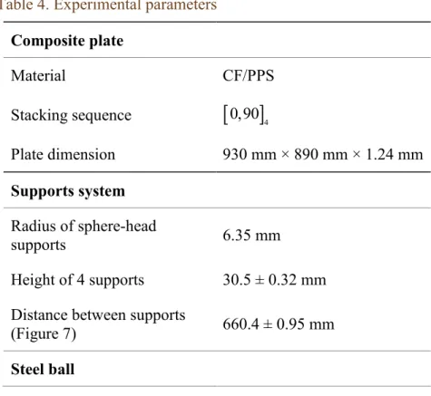
Table 4. Experimental parameters Composite plate Material CF/PPS Stacking sequence



0,90



4 Plate dimension 930 mm × 890 mm × 1.24 mm Supports system Radius of sphere-head supports 6.35 mm Height of 4 supports 30.5 ± 0.32 mm Distance between supports

(Figure 7) 660.4 ± 0.95 mm

10 Radius of steel ball 49.5 mm

Weight of steel ball 3.63 kg Deviation of ball position

from the center point (Figure

7) ±2.15 mm

Table 4 summarizes experimental parameters used in this work. The material used here is the same as the material used in the three point bending test presented above. The thickness of the four-layer laminate is 1.24 mm (0.31 mm/four-layer) with the stacking sequence



0,90 . A plate with



₄ dimensions 930 mm × 890 mm ×1.24 mm was used. This plate lies on four rigid sphere-head supports and undergoes bending deformation imposed by a 3.63 kg ball applied at center point (see Figure 7). The vertical displacement of the plate was measured using a Faro arm at 110 points on the plate surface. Three measurements were performed to get average values. The deviation values of the measurement at these points are depicted in Figure 8. The maximum deviation value is about 1.24 mm which corresponds to a maximum relative error of 5.42%.

[insert Figure 7]

Figure 7. Bending load test set-up.

[insert Figure 8]

Figure 8. Measurement deviation of vertical displacement (mm).

Test simulation and result discussion

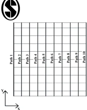
A finite element computational procedure which corresponds to the plate bending test introduced in the previous section is developed with Abaqus using a user-defined material with parameters shown in Table 2 and Table 3. The element type used in Abaqus is shell element (S4R) with a 4 layers composite section. The specimen lies on 4 rigid spheres which represent supports used in the experiment. Frictionless contact between the specimen and supports is defined. A 35.59 N load, which is equivalent to the weight of the steel ball, is applied on the plate at the same location as in the experimental test (at center point). The experimental data and simulated results were compared in terms of bending displacement along the ten paths shown in Figure 9. The comparison of experimental and simulated vertical displacement along these paths is presented in Figure 10. The maximum and minimum differences between experimental and numerical results are summarized in Table 5.

[insert Figure 9]

Figure 9. Path positions along Y axis.

Figure 10 shows that at the middle of the plate (paths 4 - 8), the simulation gives better agreement with the experimental data than on the contour of the plate (paths 1 - 3 and paths 8 - 10). The maximum difference between simulation and experiment, 6.56 mm for strain energy functions

11 in Eq.(16) and 7.87 mm for strain energy function in Eq.(17) appears at the boundary of the plate (path 1) (see Table 5).

The average discrepancies between experimental and numerical results are 3.64 mm and 3.39 mm respectively for the strain energy functions in Eqs.(16) and (17), which are quite small in comparison to the dimensions of the composite sheet. It demonstrates that the simulations with two orthotropic hyperelastic models used in this study gave good agreements with the experimental results. It is remarked that the strain energy function of Eq.(17) provided better response than that of Eq.(16).

[insert Figure 10]

Figure 10. Result comparison ((a) Path 1, (b) Path 2, (c) Path 3, (d) Path 4, (e) Path 5, (f) Path 6, (g)

Path 7, (h) Path 8, (i) Path 9, (j) Path 10).

Table 5. Maximum and minimum difference in vertical displacement between experimental and simulation data on each path

Path

Strain energy function in

Eq.(16) Strain energy function in Eq.(17) Min (mm) Max (mm) Min (mm) Max (mm)

Path 1 1.53 6.56 0.31 7.87 Path 2 1.34 5.44 0.04 6.56 Path 3 1.43 4.56 0.17 5.36 Path 4 1.14 2.81 0.24 3.39 Path 5 0.47 2.78 0.16 2.92 Path 6 0.79 2.73 0.38 2.15 Path 7 1.66 2.84 0.26 3.55 Path 8 1.43 4.57 0.15 5.17 Path 9 1.191 5.22 0.27 6.10 Path 10 0.50 4.62 0.08 5.86

Conclusion

This paper presents the implementation of two orthotropic hyperelastic models used for assessing the mechanical behavior of multi-layer FRTPC sheets. These models were developed based on the

12 polyconvexity condition of strain energy function and implemented in the user-defined material subroutine of Abaqus for finite strain shell elements. The material parameters were numerically identified by fitting numerical simulation results to experimental results obtained from three bending tests for both stacking sequences



0,90 and



₄

 

45 ₄. These models were then validated through the ball load test on a large composite sheet. Results showed that:

 Both proposed orthotropic hyperelastic models are appropriate for the CF/PPS multi-layer composite material.

 The parameters of these models can be well identified in three point bending tests with two different fiber orientation configurations.

 The numerical simulation using shell element (S4R) with the composite section of 4 layers in Abaqus is good enough for the multi-layer FRTPC sheets.

 These material models responded well the validation case of the ball load test on a large CF/PPS multi-layer composite sheet.

Acknowledgments

The authors would like to thank the National Sciences and Engineering Research Council (NSERC) and our industrial partners for their support and financial contribution.

Declaration of conflicting interests

The author(s) declared no potential conflicts of interest with respect to the research, authorship, and/or publication of this article.

References

1. Abenhaim GN, Tahan AS, Desrochers A, et al. A Novel Approach for the Inspection of Flexible Parts Without the Use of Special Fixtures. J Manuf Sci Eng 2011; 133: 011009-011009-011011.

2. Abenhaim GN, Desrochers A and Tahan A. Nonrigid parts’ specification and inspection methods: notions, challenges, and recent advancements. Int J Adv Manuf Technol 2012; 63: 741-752.

3. Aidibe A, Tahan AS and Abenhaim GN. Distinguishing profile deviations from a part’s deformation using the maximum normed residual test. WSEAS Transactions on Applied and Theoretical Mechanics 2012; 7: 11.

13 4. Aidibe A and Tahan A. Adapting the coherent point drift algorithm to the fixtureless

dimensional inspection of compliant parts. Int J Adv Manuf Technol 2015; 79: 831-841. 5. Abenhaim GN, Desrochers A, Tahan AS, et al. A virtual fixture using a FE-based

transformation model embedded into a constrained optimization for the dimensional inspection of nonrigid parts. Comput-Aided Des 2015; 62: 248-258.

6. Sabri V, Tahan SA, Pham XT, et al. Fixtureless profile inspection of non-rigid parts using the numerical inspection fixture with improved definition of displacement boundary conditions. Int J Adv Manuf Technol 2016; 82: 1343-1352.

7. Sattarpanah Karganroudi S, Cuillière J-C, Francois V, et al. Automatic fixtureless inspection of non-rigid parts based on filtering registration points. Int J Adv Manuf Technol 2016; 87: 687-712.

8. Gruttmann F and Taylor RL. Theory and finite element formulation of rubberlike membrane shells using principal stretches. Int J Numer Methods Eng 1992; 35: 1111-1126.

9. Weiss JA, Maker BN and Govindjee S. Finite element implementation of incompressible, transversely isotropic hyperelasticity. Comput Methods Appl Mech Eng 1996; 135: 107-128. 10. Prot V, Skallerud B and Holzapfel GA. Transversely isotropic membrane shells with application to mitral valve mechanics. Constitutive modelling and finite element implementation. Int J Numer Methods Eng 2007; 71: 987-1008.

11. Itskov M. A generalized orthotropic hyperelastic material model with application to incompressible shells. Int J Numer Methods Eng 2001; 50: 1777-1799.

12. Tanaka M, Noguchi H, Fujikawa M, et al. Development of Large Strain Shell Elements for Woven Fabrics with Application to Clothing Pressure Distribution Problem. Computer Modeling in Engineering & Sciences 2010; 62, No.3: 265-290.

13. Spencer AJM. Theory of fabric-reinforced viscous fluids. Composites Part A 2000; 31: 1311-1321.

14. Balzani D, Neff P, Schröder J, et al. A polyconvex framework for soft biological tissues. Adjustment to experimental data. Int J Solids Struct 2006; 43: 6052-6070.

15. Holzapfel GA, Gasser TC and Ogden RW. A New Constitutive Framework for Arterial Wall Mechanics and a Comparative Study of Material Models. J Elast 2000; 61: 1-48.

16. Nolan DR, Gower AL, Destrade M, et al. A robust anisotropic hyperelastic formulation for the modelling of soft tissue. J Mech Behav Biomed Mater 2014; 39: 48-60.

14 17. Pham X-T, Bates P and Chesney A. Modeling of Thermoforming of Low-density Glass Mat

Thermoplastic. J. Reinf. Plast. Compos. 2005; 24: 287-298.

18. Peng XQ, Guo ZY, Zia-Ur-Rehman, et al. A Simple Anisotropic Fiber Reinforced Hyperelastic Constitutive Model for Woven Composite Fabrics. Int J Mater Form 2010; 3: 723-726.

19. Suchocki C. A Finite Element Implementation of Knowles Stored-Energy Function: Theory, Coding and Applications. Archive of Mechanical Engineering 2011; 58: 319.

20. Holzapfel GA. Nonlinear solid mechanics: A continuum approach for engineering. Chichester: Wiley, 2000.

21. Abaqus. Using Abaqus Online Documentation, Version 6.13, Dassault Systèmes Simulia Corp., Providence, RI, USA, http://129.97.46.200:2080/v6.13 (2013, accessed 26 September 2016).

22. Simo JC and Hughes TJR. Computational Inelasticity. Springer-Verlag New York, 1998, p.XIV, 392.

15

16

17

18

19

20

Fig. 16 Comparison between numerical results and experimental data: a) strain energy function in Eq.(16); b) strain energy function in Eq.(17).

21

22

23

24

Fig. 20 Result comparison ((a) Path 1, (b) Path 2, (c) Path 3, (d) Path 4, (e) Path 5, (f) Path 6, (g) Path 7, (h) Path 8, (i) Path 9, (j) Path 10).