HAL Id: hal-01796028
https://hal-amu.archives-ouvertes.fr/hal-01796028
Submitted on 18 May 2018
HAL is a multi-disciplinary open access
archive for the deposit and dissemination of
sci-entific research documents, whether they are
pub-lished or not. The documents may come from
teaching and research institutions in France or
abroad, or from public or private research centers.
L’archive ouverte pluridisciplinaire HAL, est
destinée au dépôt et à la diffusion de documents
scientifiques de niveau recherche, publiés ou non,
émanant des établissements d’enseignement et de
recherche français ou étrangers, des laboratoires
publics ou privés.
A Simple Data Cube Representation for Efficient
Computing and Updating
Viet Phanluong
To cite this version:
Viet Phanluong. A Simple Data Cube Representation for Efficient Computing and Updating.
Inter-national Journal On Advances in Intelligent Systems, IARIA, 2016, pp.2016 - 2016. �hal-01796028�
A Simple Data Cube Representation for
Efficient Computing and Updating
Viet Phan-Luong
Aix-Marseille Universit´eLaboratoire d’Informatique Fondamentale de Marseille LIF - UMR CNRS 7279
Marseille, France
Email:[email protected]
Abstract—This paper presents a simple approach to represent
data cubes that allows efficient computing, querying and updat-ing. The representation is based on (i) a recursive construction of the power set of the scheme of the fact table and (ii) a prefix tree structure for the compact storage of cuboids. The experimental results on large real datasets show that the approach is efficient in run time, storage space, and for incremental update.
Keywords–Data warehouse; Data mining; Data cube; Data cube update.
I. INTRODUCTION
In data warehouse, a data cube built on a fact table with n dimensions and m measures can be seen as the result of the set of the Structured Query Language (SQL) group-by queries over the power set of dimensions, with aggregate functions over the measures. The result of each SQL group-by query is an aggregate view, called a cuboid, over the fact table. The concept of data cube, provided in the online analytical processing (OLAP) approach, offers important interests to business intelligence as it provides aggregate views of data over multiple combinations of dimensions that help managers to make appropriate decision in their business.
Though the concept of data cube is simple, there are many important issues in computation. In fact, in a data warehouse, the fact table has generally a big volume. This implies the cost in time and in storage space, when computing the cuboids. As the number of cuboids in a data cube is exponential with respect to the number of dimensions of the fact table, the cost to compute the entire data cube is considerable.
To improve the query response time on data cube, in OLAP, the data cube is usually precomputed and stored on disks. However, the storage space of all the data cube is exponential to the number of dimensions of the fact table. For efficiency, it is necessary to reduce the storage space. By reduction, the data cube is represented in a compact form that is stored on disks. We must access this form to compute the response to queries on data cube. There exists the trade-off between the storage space reduction and the query response time. The reduction of the storage space could increase the query response time. The research in OLAP focuses on the important efforts to make methods more efficient in computation and representation of data cubes. The compact representation of data cubes should offer efficient query computation.
In the life cycle of a data warehouse, the fact table can incrementally grow with new fact tuples. In consequence, the data cube must be updated. The update can be done by updating the stored representation based on the new data or by re-computing the entire representation of the data cube based on the updated fact table. On updating all cuboids, we can have the same problems as on re-computing all cuboids. However, it is interesting to know between the two possibilities, in what conditions, which one is more efficient than the other.
Further more, because of the big volume of the fact table and the exponential number of cuboids, we can have a tremendous number of aggregated tuples in the data cube. As consequence, the apprehension on such a number of aggregated tuples to make a good decision on business is a very important issue.
The above issues are among the important topics of re-search in data warehouse. There exist many approaches to compute and to represent the data cube. The work [1] presents a new approach to represent the data cube that is efficient in storage space and in computing. By this approach, the storage space of the data cube representation is reduced. However, we can have an efficient method to get all cuboids of the entire data cube from the reduced representation.
This work is an extension of [1]. The extension consists in: (i) development and improvement of the content and (ii) the study of data cube update based on the proposed representation.
The paper is organized as follows. Section II presents the related work and the contributions of this work. Section III introduces the concepts of the prime and next-prime schemes and cuboids. Section IV presents the structure of the integrated binary search prefix tree used to store cuboids. Section V is the core of the approach. It shows how to compute the data cube representation and how to restore the entire data cube from the reduced representation. Section VI presents an efficient algorithm for updating the data cube representation. Section VII reports the experimentation results. Finally, conclusion and further work are in Section VIII.
II. RELATED WORK
To tackle the issues of the tremendous number of aggre-gated tuples of a data cube due to the big volume of the fact table and the exponential number of cuboids [2][3][4][5],
many different approaches were proposed. In [6], instead of computing the complete data cube, an I/O-efficient technique based upon a multiresolution wavelet decomposition is used to build an approximate and space-efficient representation of the data cube. To answer an OLAP query, instead of computing the exact response, an approximate response is computed on this representation.
Iceberg data cube [7][8][9][10] is another approach to build incomplete data cube. In this approach, instead of computing all aggregated tuples, only those with support (or occurrence frequency) greater than certain thresholds are computed for the data cube. For efficient computation, the pruning technique in the search space is enforced based on anti-monotone con-straints. This approach does not allow to answer all OLAP queries, because the data cube is partially computed.
To be able to answer all OLAP queries, many researchers focused the efforts to find the methods to represent the entire data cube with efficient computation and storage space. To reduce the time computing and the storage space, several interesting data structures were created. Dwarf data structure [11][12] is a special directed acyclic graph that allows not only the reduction of redundancies of tuple prefixes as the prefix tree structure, but also the reduction of tuple suffixes by coalescing the same tuple suffixes, using pointers. In addition Dwarf is a hierarchical structure that allows to store tuples and their subtuples on the same path of the graph, using the special key value ALL. Using Dwarf data structure for data storage, the exponential size of data cube is reduced dramatically. However, this structure is not relational and then cannot be directly apply in OLAP based on relational database tools (ROLAP).
In ROLAP, data cube is represented in relational tables. To be able to rapidly answer data cube queries, aggregate tables can be precomputed and stored on disks. To optimize the storage space, the aggregated tuples that can be deduced from already stored tuples are not stored, but represented by references to stored tuples. The reduction of the redundancies between tuples in cuboids is based on equivalence relations defined on aggregate functions [13][14] or on the concept of closed itemsets in frequent itemset mining [15][16].
The computation of all cuboids is usually organized on the complete lattice of subschemes of the dimension scheme of the fact table, in such a way the run time and the storage space can be optimized by reducing redundancies [3][13][14][17][18]. The computation can traverse the complete lattice in a top-down or bottom-up manner [9][19][20]. For grouping tuples to create cuboids, the sort operation can be used to reorganize tuples: tuples are grouped over the prefix of their scheme and the aggregate functions are applied to the measures. By group-ing tuples, the fact table can be horizontally partitioned, each partition can be fixed in memory, and the cube computation can be modularized.
The top-down methods [19][20] walk the paths from the top to the bottom in the complete lattice, beginning with the node corresponding to the largest subscheme (the dimension scheme of the fact table, for the first processed path). To optimize the data cube construction, the cuboids over the subschemes on a path from the top to the bottom in the complete lattice can be built in only one lecture of the fact table. For this, an aggregate filter (accumulator), initialized with an empty tuple and a non aggregated mark, is used for
each subscheme on the path. Each filter contains, at each time, only one tuple over the subscheme (associated with the filter) and the current aggregate value of the measure (or a non aggregated mark). Before processing, the tuples of the fact table are sorted over the largest scheme of the path. When reading the new tuple of the fact table, if over a subscheme of the currently processed path, the new tuple has the same value as the tuple in the filter, then only the aggregate value of the measure is updated. Otherwise, the current content of the filter is flushed out to the file of the corresponding cuboids on disk, and before the new tuple passes into the filter, the subtuple of the current content, over the next subscheme of the currently processed path (from the top to the bottom), is processed as the new tuple of the next subscheme filter. The same process is recursively applied to the subsequent subscheme filters.
To optimize the storage space of a cuboid, only aggregated subtuples with aggregate value of measure are directly stored on disk. Subtuples with non-aggregated mark are not stored but represented by references to the (sub)tuples where the non aggregated tuples are originated. Consequently, to answer a data cube query, by this representation, we may need to access to many different stored cuboids.
The bottom-up methods [13][14][17][20] walk the paths from the bottom to the top in the complete lattice, beginning with the empty node (corresponding to the cuboid with no dimension, for the first processed path). For each path, let T0
be the scheme at the bottom node and Tnthe scheme at of the
top node of the path (not necessary the bottom and the top of the lattice, as each node is visited only once). These methods begin by sorting the fact table over T0 and by this, the fact
table is partitioned into groups over T0. To optimize storage
space, for each one of these groups, the following depth-first recursive process is applied.
If the group is single (having only one tuple), then the only element of the group is represented by a reference to the corresponding tuple in the fact table, and there is no further process: the recursive cuboid construction is pruned.
Otherwise, an aggregated tuple is created in the cuboid over
T0 and the group is sorted over the next larger scheme T1 on
the path. The group is then partitioned into subgroups over T1.
For each subgroup over T1, the creation of a real tuple or a
reference is similar to what we have done for a group over T0.
When the recursive process is pruned at a node Ti,0 ≤
i≤ n, or reaches to Tn, it resumes with the next group of the
partition over T0, until all groups of the partition are processed.
The construction resumes with the next path, until all paths of the complete lattice are processed, and all cuboids are built.
Note that in the above optimized bottom-up method, in all cuboids, if references exist, they refer directly to tu-ples in the fact table, not to tutu-ples in other cuboids. This method, named Totally-Redundant-Segment BottomUpCube (TRS-BUC), is reported in [20] as a method that dominates or nearly dominates its competitors in all aspects of the data cube problem: fast computation of a fully materialized cube in compressed form, incrementally updateable, and quick query response time.
For updating a data cube with new tuples coming into the fact table, we can find in [20] the implementation of three update methods. (i) Merge method: build the data cube of the new tuples and then merge it with the current data
cube. (ii) Direct method: update each cuboid of the current data cube with the new tuples. (iii) Reconstruction method: reconstruct the entire data cube of the fact table updated with the new tuples. These methods are experimented on different approaches to incrementally build the data cube, where the size of new dataset grows gradually from 1% to 10% of the size of the current fact table.
In the above approaches, the traversal of the complete lattice of the cuboids and the reduction of tuple redundancy by references imply the dependencies between cuboids. This can impact on the query response time and/or on the data cube update. Moreover, the representation of the entire data cube is computed for a specific measure and a specific aggregate function. When we need to have aggregate views on other measures and/or on other aggregate functions, we need to rebuild the data cube. To improve the query response time or the update time, indexes can be created for cuboids. Because of the tremendous number of aggregated tuples in the exponential number of cuboids, the time consuming for index creation may much longer than the time for building the data cube. A. Contributions
This paper is an extension of the paper [1] that presents a simple and efficient approach to compute and to represent the entire data cubes. The extension consists in: (i) development and improvement of the contents (points 1 to 4 in what follows), and (ii) the implement of data cube update (point 5).
The efficient representation of data cube is not only a compact representation of all cuboids of the data cube, but also an efficient method to get the entire cuboids from the compact representation. The representation also allows to efficiently update the data cube when new data come into the fact table. The main ideas and contributions of the proposed approach are:
1) Among the cuboids of a data cube, there are ones that can be easily and rapidly get from the others, with no important computing time. We call these others the prime and next-prime cuboids.
2) The prime and next-prime cuboids are computed and stored on disk using a prefix tree structure for compact representation. To improve the efficiency of search through the prefix tree, this work integrates the binary search tree into the prefix tree.
3) To compute the prime and next-prime cuboids, this work proposes a running scheme in which the com-putation of the current cuboids can be speeded up by using the cuboids that are previously computed. 4) Based on the prime and next-prime cuboids that are
stored on disks, an efficient algorithm is proposed to retrieve all other cuboids that are not stored. 5) To update the data cube, we need only to update the
prime and next-prime cuboids. An efficient algorithm for updating data cube is presented and experimented. To compute the aggregates, this approach does not need to sort the fact table or any part of it beforehand. To optimize the computation and the storage space, the approach is not based on the complete lattice of subschemes of the dimension scheme and does not use sophisticated techniques to implement direct or indirect references of tuples in cuboids. Hence, there are no
dependencies between the cuboids in the representation that can impact on query response time or on data cube update. Moreover, in contrast to the existing approaches in which the compact data cube is computed for a specific measure and a specific aggregate function and, to improve the query response time, the index can be created for data in the cuboids later, this approach prepares the data cube for any measure and any aggregate function by creating the cube of indexes.
III. PRIME AND NEXT-PRIME CUBOIDS
This section defines the main concepts of the present approach to compute and to represent data cubes.
A. A structure of the power set
A data cube over a dimension scheme S is the set of cuboids built over all subsets of S, that is the power set of S. As in most of existing work, attributes are encoded in integer, let us consider S = {1, 2, ..., n}, n ≥ 1. The power set of S
can be recursively defined as follows.
1) The power set of S0= ∅ (the empty set) is P0= {∅}.
2) For n≥ 1, the power set of Sn = {1, 2, ..., n} can
be recursively defined as follows:
Pn= Pn−1∪ {X ∪ {n} | X ∈ Pn−1} (1)
Pnis the union of Pn−1(the power set of Sn−1) and
the set of which each element is got by adding n to each element of Pn−1.
Let us call Pn−1 the first-half power set of Sn and
the second operand of Pn the last-half power set of
Sn.
As the number of subsets in Pn−1 is 2n−1, the number of
subsets in the first-half power set of Sn is 2n−1. As each
subset in the last-half power set of Sn is obtained by adding
element n to a unique subset of the first-half power set of Sn,
the number of subsets in the last-half power set of Sn is also
2n−1. Every subset in the first-half power set does not contain
n, but every subset in the last-half power set does contain n.
Moreover, the subsets in the last-half power set can be divided in two groups: one contains the subsets having element 1 and the other contains the subsets without element 1.
Example 1: For n= 3, S3= {1, 2, 3}, we have:
P0= {∅}; P1= {∅, {1}}; P2= {∅, {1}, {2}, {1, 2}};
P3= {∅, {1}, {2}, {1, 2}, {3}, {1, 3}, {2, 3}, {1, 2, 3}}.
The first-half power set of S3 is:
{∅, {1}, {2}, {1, 2}}.
And the last-half power set of S3 is:
{{3}, {1, 3}, {2, 3}, {1, 2, 3}}.
B. Last-half data cube and first-half data cube
Consider a fact table R (a relational data table) over a dimension scheme Sn= {1, 2, ..., n}. In view of the first-half
and the last-half power set, suppose that X = {x1, ..., xi} is an
element of the first-half power set of Sn ({x1, ..., xi} ⊆ Sn).
Let Y be the smallest element of the last-half power set of
Sn that contains X. Then, Y = X ∪ {n}. If the cuboid over
Y is already computed in the attribute order x1, ..., xi, n, then
sequential reading of the cuboid over Y to get data for the cuboid over X. So, we define the following concepts.
– We call a scheme in the last-half power set a prime scheme and a cuboid over a prime scheme a prime cuboid. Note that all prime schemes contain the last attribute n and any scheme that contains attribute n is a prime scheme.
– For efficient computing, the prime cuboids can be com-puted by pairs. Such a pair is composed of two prime cuboids. The scheme of the first one has attribute 1 and the scheme of
the second one is obtained from the scheme of the first one by deleting attribute 1. We call the second prime cuboid the
next-prime cuboid.
– The set of all cuboids over the prime (or next-prime) schemes is called the last-half data cube. The set of all remaining cuboids is called the first-half data cube. In this approach, the last-half data cube is computed and stored on disks. Cuboids in the first-half data cube are computed as queries based on the last-half data cube.
IV. INTEGRATED BINARY SEARCH PREFIX TREE
The prefix tree structure offers a compact storage for tuples: the common prefix of tuples is stored once. So, there is no redundancy in storage. Despite the compact structure of the prefix tree, if the same prefix has a large set of different suffixes, then the time for searching the set of suffixes can be important. To improve the search time when building the prefix tree, this work proposes to integrate the binary search tree into the prefix structure. The integrated structure, called the binary search prefix tree (BSPT), is used to store tuples of cuboids. With this structure, tuples with the same prefix are stored as follows:
– The prefix is stored once.
– The suffixes of those tuples are organized in siblings and stored in a binary search tree.
Precisely, in C language, the structure is defined by : typedef struct bsptree Bsptree; // Binary search prefix tree struct bsptree{ Elt data; // data at a node
Ltid *ltid; // list of RowIds Bsptree *son, *lsib, *rsib;};
where son, lsib, and rsib represent respectively the son, the left and the right siblings of nodes. The field ltid is reserved for the list of tuple identifiers (RowId) associated with nodes. For efficient memory use, ltid is stored only at the last node of each path in the BSPT.
With this representation, each binary search tree contains all siblings of a node in the normal prefix tree.
Example 2:
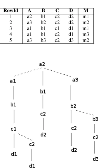
Consider Table I that represents a fact table R1 over the dimension scheme ABCD and a measure M . Fig. 1 represents the BSPT of the tuples over the scheme ABCD of the fact table R1, where we suppose that with the same letter x, if
i < j then xi < xj, e.g., a1 < a2 < a3. In this figure, the
continuous lines represent the son links and the dashed lines represent the lsib or rsib links.
In each binary search tree of Fig. 1, if we do the depth-first search in in-order, we can get tuples in increasing order as follows:
TABLE I. FACT TABLE R1
RowId A B C D M 1 a2 b1 c2 d2 m1 2 a3 b2 c2 d2 m2 3 a1 b1 c1 d1 m1 4 a1 b1 c2 d1 m3 5 a3 b3 c2 d3 m2
Figure 1. A binary search prefix tree
(a1, b1, c1, d1) (a1, b1, c2, d1) (a2, b1, c2, d2) (a2, b2, c2, d2) (a2, b3, c2, d3)
The BSPT is saved to disk with the following format:
level: suf f ix : ltid
where
– level is the length of the prefix part that the path has in common with its left neighbor,
– suffix is tuple (a list of dimension values) and, – ltid is a list of tuple identifiers (RowId).
Cuboids are built using the BSPT structure. The list of RowIds associated with the last node of each path allows the aggregate of measures. For example, with the fact table in Table I, the cuboid over ABCD is saved on disk as the following. 0 : a1 b1 c1 d1 : 3 2 : c2 d1 : 4 0 : a2 b1 c2 d2 : 1 0 : a3 b2 c2 d2 : 2 1 : b3 c2 d3 : 5 A. Insertion of tuples in a BSPT
The following algorithm, named Tuple2Ptree, defines the method to insert tuples into a BSPT, while maintaining the BSPT structure.
Algorithm Tuple2Ptree: Insert a tuple into a BSPT.
Input: A BSPT represented by node P , a tuple ldata and its list of RowIds lti.
Output: The tree P updated with ldata and lti. Method:
If P is null then
create P with P->data = head(ldata); P->son = P->lsib = P->rsib = NULL; if queue(ldata) is null then P->ltid =lti;
else P->son = Tuple2Pree(P->son, queue(ldata), lti); Else if P->data > head(ldata) then
P->lsib=Tuple2Ptree(P->lsib, ldata,lti); else if P->data < head(ldata) then
P->rsib=Tuple2Ptree(P->rsib, ldata,lti); else if queue(ldata) is null then
P->ltid = append(P->ltid, lti);
else P->son = Tuple2Ptree(P->son, queue(ldata), lti); return P;
In the Tuple2Ptree algorithm, head(ldata) returns the first
element of ldata, queue(ldata) returns the queue of ldata
after removing head(ldata), and append(P ->ltid, lti) adds
the list lti to the list of RowIds associated with node P . B. Grouping tuples using binary prefix tree
To create the BSPT of a table of tuples where each one has a list of RowIds lti, we use an algorithm named Table2Ptree. This algorithm allows to group the tuples over the dimension scheme of the table, hence allows to create the corresponding cuboid. As nodes corresponding to each attribute of tuples are organized in binary search tree structures, we can get the cuboid with groups of tuples ordered in the increasing order. Algorithm Table2Ptree: Build a BSPT for a relational table. Input: A table R in which each tuple has a list of tids lti. Output: The BSPT P for R
Method:
Create an empty BSPT P;
For each tuple ldata in R with its list of tids lti do P = Tuple2Ptree(P, ldata, lti); done;
Return P;
V. THE LAST-HALF DATA CUBE REPRESENTATION
This section presents a method to build the last-half data cube. It also shows how the data cube is represented by the last-half data cube and how the entire data cube can be restored from this representation.
A. Computing the last-half data cube
Let S = {1, 2, ..., n} be the set of all dimensions of the
fact table. To compute all prime and next-prime cuboids of the last-half data cube, we process as follows:
– Based on the fact table, we begin by computing the first pair of prime and next-prime cuboids, one over S and the other over S− {1}.
– In the sequence, based on the previously computed pairs of prime and next-prime cuboids we compute the other pairs
of prime and next-prime cuboids. To control the computation, we use:
(i) A list to keep track of the generated prime schemes. This list is called the running scheme and denoted by RS and, (ii) A current scheme, denoted by cS, that is set to a prime scheme that is currently considered in RS. From the current scheme, the further pairs of prime and next-prime cuboids are generated, based on the cuboid over the current scheme.
Through the computation of the last-half data cube, after the generation of the first pair of prime and next-prime cuboids, the dimension scheme S is the first prime scheme added into
RS and cS is initialized to S. Then, for each dimension d, d6= 1 and d 6= n, the prime scheme cS − {d} is generated. If cS− {d} is not yet in RS, then it is appended to RS and we
compute the pair of prime and next-prime cuboids, one over
cS− {d} and the other over cS − {1, d}, based on the cuboids
over cS. When all dimensions d ∈ cS, d 6= 1, d 6= n are
considered, cS is set to the next scheme in RS for generating new pairs of prime and next-prime cuboids. The process ends when all prime schemes of size k >2 in RS are treated.
We associate each prime scheme X in RS with information that allows to retrieve the pairs of prime cuboids over X and
X− {1}. This is not only necessary when computing the
last-half data cube, but also when restoring the entire data cube. More formally, we use the following algorithm, named
LastHalf Cube, for computing the last-half data cube.
Algorithm LastHalfCube
Input: A fact table R over scheme S of n dimensions. Output: The last-half data cube of R and the running scheme
RS.
Method:
0) Initialize the list RS to emptyset; 1) Append S to the RS;
2) Generate two prime and next-prime cuboids over S and S -{1}, respectively, using algorithm Table2Tree and R;
3) Set cS to the first scheme in RS; // cS: current scheme 4) While cS has more than 2 attributes do
5) For each dimension d in cS, d6= 1 and d 6= n, do
6) Build a subscheme scS by deleting d from cS; 7) If scS is not yet in RS then append scS to RS and let
Cubo be the already computed cuboid over cS; 8) Using Table2Ptree and Cubo to generate two
cuboids over scS and scS - {1}, respectively;
9) done;
10) Set cS to the next scheme in RS; 11) done;
12) Return RS;
Example 3: An example of running scheme.
Table II shows the simplified execution of the LastHalfCube algorithm on a fact table R over the dimension scheme S = {1, 2, 3, 4, 5}. In this table, only the prime
and the next-prime (NPrime) schemes of the cuboids computed by the algorithm are reported. The prime schemes appended to the Running Scheme RS during the execution
of LastHalfCube are in the columns named Prime/RS. The first prime schemes are in the first column Prime/RS, the next ones are in the second column Prime/RS, and the final ones are in the third column Prime/RS. The final state of RS is
{12345, 1345, 1245, 1235, 145, 135, 125, 15}. In Table II, the
schemes marked with x (e.g., 145x) are those already added to RS and are not re-appended to RS.
TABLE II. GENERATION OF THE RUNNING SCHEME OVER S ={1, 2, 3, 4, 5}.
Prime NPrime Prime NPrime Prime NPrime
RS RS RS 12345 2345 1 345 345 1 45 45 15 5 1 35 35 15x 12 45 2 45 1 45x 1 25 25 15x 123 5 23 5 1 35x 1 25x
Proof of correctness and soundness. To prove the correctness and soundness of the LastHalfCube algorithm, we only need to show that for a fact table R over a scheme S of n dimensions,
S = {1, 2, ..., n}, the LastHalfCube algorithm generates RS
with 2n−2 subschemes containing 1 and n as the first and
the last attributes. For this, we can see that all subschemes appended to RS have1 as the first attribute and n as the last
attribute. So, we can forget1 and n from all those subschemes.
Therefore, we can consider that the first subscheme added to RS is 2, ..., n − 1. Over 2, ..., n − 1, we have only one
subscheme of size n− 2 (Cn−2
n−2= 1). In the loop For at point
5 of the LastHalfCube algorithm, alternatively each attribute from 2 to n− 1 is deleted to generate a subscheme of size n− 3. By doing this, we can consider as, in each iteration,
we build a subscheme over n− 3 different attributes selected
among n− 2 attributes. So, we build Cn−3
n−2 subschemes. So
on, until the subscheme {1, n} (corresponding to the empty
scheme after forgetting 1 and n) is added to RS. We have: Cn−2n−2+ Cn−2n−3+ .... + C0
n−2= 2n−2
For each of these 2n−1 prime schemes, the LastHalfCube
algorithm also computes the corresponding next-prime scheme. By adding the 2n−2 corresponding next-prime schemes, we
have 2n−1 different subschemes. Thus, the LastHalfCube
al-gorithm computes 2n−1 prime and next-prime schemes (and
cuboids).
B. Data Cube representation
For a fact table R over a dimension scheme S = {1, 2, ..., n} with measures M1, ..., Mk, the data cube of R
is represented by (RS, LH, F ), where
1) RS is the running scheme, i.e., the list of all prime schemes over S. Each prime scheme has an identifier number that allows to locate the files corresponding to the prime and next-prime cuboids in the last-half data cube.
2) LH: The last-half data cube of which the cuboids are precomputed and stored on disks using the format to store the BSPT.
3) F : A relational table over RowId, M1, ..., Mk that
represents the measures associated with each tuple of R. Clearly, such a representation reduces about 50% space of the entire data cube, as it represents the last-half data cube in the BSPT format.
C. Computing the first-half data cube
In this subsection, we show how the cuboids of the first-half data cube are computed based on the last-first-half data cube. Let S= {1, 2, ..., n} be the dimension scheme of the data
cube and X = {xi1, ..., xik} be the scheme of a cuboid in the
first-half data cube that we need to retrieve. The size of X is
k (k < n, n6∈ X); n is the size of S and also the last attribute
of S.
Let C be the stored cuboid over X∪ {n} (C is in the
last-half data cube). C is a prime cuboid if X contains attribute
1, a next prime cuboid, if not. Remind from Section IV that a
tuple of a prime or next-prime cuboid is stored on disk in the BSPT format:
level: suf f ix : ltid
By BSPT structure, the tuples of C that have the same prefix over X are already regrouped together when C is stored on disk. For each such a group, we take the prefix and the collection of all tuple identifiers (RowId) in the lists of identifiers associated with these tuples to create a record (an aggregated tuple) of the cuboid over X. More formally, to build the cuboid over X, we use the following algorithm named Aggregate-Projection.
Algorithm Aggregate-Projection
Input: The representation (RS, LH, F ) of a data cube over a
dimension scheme S = {1, 2, ..., n} and a scheme X of size k, such that n6∈ X.
Output: The cuboid over X of the data cube represented by
(RS, LH, F ).
Method:
Let C be the prime cuboid over X∪ {n};
// C is precomputed and stored in LH.
Let level: suf f ix, t(n) : ltid be the 1st record in C;
// t(n): the tuple value at attribute n. As the 1st record in C,
// we have level= 0 and suf f ix is a tuple of size k.
Set tc = suf f ix; ltidc= ltid;
//(tc: ltidc): the record currently built for the cuboid over X
For each new record levelw: suf f ixw, tw(n) : ltidw
sequentially read in C do
If levelw≥ k, then append ltidw to the end of ltidc;
// case the new tuple of C has the same prefix as // the tuple currently built.
Else
Write tc: ltidc to disk as an aggregated tuple of
the cuboid over X;
Update the elements of the tuple tc, from rang
levelw+ 1 to rang k, with the corresponding
attribute values of the tuple suf f ixw and
Re-initialize ltic to ltidw;
D. Querying data cubes
In contrast to existing approaches, the present approach does not compute the representation of the data cube for a specific measure, neither for a specific aggregate function, but it computes the representation that is ready for the computation on any measure and any aggregate function. The last-half data cube is in fact the collection of index tables of tuples of the cuboids in the last-half data cube. We can get the cuboid over a scheme X with a specific measure M and a specific aggregate function g, based on the representation in Subsection V-B, by slightly modifying the Aggregate-Projection algorithm. The modified algorithm is named Aggregate-Query.
Algorithm Aggregate-Query
Input: The representation (RS, LH, F ) of a data cube over a
dimension scheme S = {1, 2, ..., n} and a scheme X of size k≤ n, a measure M and an aggregate function g.
Output: The cuboid over X computed for g and M . Method:
If n∈ X then
Let C be the prime cuboid∈ LH, over X;
For each record(level : suf f ix : ltid) ∈ C do,
Let t be the tuple built on level and suf f ix; Let Ω be the set of values of the measure M
computed on ltid and the relational table F ; Apply g toΩ; print (t : g(Ω));
done; Else,
Let C be the prime cuboid over X∪ {n};
Let(level : suf f ix, t(n) : ltid) be the 1st record in C;
Set tc= suf f ix; ltidc= ltid;
For each new record (levelw: suf f ixw, tw(n) : ltidw)
sequentially read in C do
If levelw≥ k then append ltidwto the end of ltidc;
Else,
Let Ω be the set of values of the measure M
computed on ltidc and the relational table F ;
Apply g toΩ; print (tc: g(Ω));
Update the elements of the tuple tc, from rang
levelw+ 1 to rang k, with the corresponding
attribute values of the tuple suf f ixwand
Re-initialize ltic to ltidw;
done.
VI. UPDATING DATA CUBES
For updating a data cube with new tuples coming into the fact table, we can have three data cube update methods. (i) The Merge method builds the data cube of the new tuples and then merge it with the current data cube. (ii) The Direct method updates each cuboid of the current data cube with the new tuples. (iii) The Reconstruction method reconstructs the entire data cube of the fact table updated with the new tuples.
In the present approach, a data cube is represented by its last-half. When new data coming into the fact table, to update the data cube, we need only to update its last-half. The three methods of data cube update can be applied to the representation by the last-half data cube. In particular, the Merge method and the Direct method can be more efficient with the last-half data cube representation: we must only merge or access to a half number of cuboids of the data
cube. Moreover, as we do not walk the complete lattice of the cuboids in the data cube, we can update each cuboid independently.
The present work has implemented the update by the Direct method. For this, the cuboids of the current last-half data cube are restored from disk to main memory, in the binary search prefix tree structure. For each such a restored tree, the projection of new data on the scheme of the cuboid stored in the tree is inserted into the tree. Precisely, we use the following algorithm, named LastHalfCubeUpdate, to update the last-half cube.
Algorithm LastHalfCubeUpdate: Update the last-half data cube with new data tuples.
Input: The representation(RS, LH, F ) of a data cube, where RS is the running scheme, LH the last-half data cube, F the
current fact table, and a new fact table N F .
Output: The updated representation (RS, LH′, F ∪ N F )
where LH′ is the last-half data cube of the updated fact table
F ∪ N F .
Method:
For each Sch in the running scheme RS do
1) From the last-half cube LH, restore the prime cuboid associated with Sch in a BSPT;
2) For each tuple t of the new fact table N F , insert the restriction of t on Sch (i.e., t[Sch]) into the BSPT of the prime
cuboid using the Tuple2Ptree algorithm; 3) Save the BSPT to disk;
4) From the last-half cube LH, restore the next-prime cuboid associated with Sch− {1} in a BSPT;
5) For each tuple t of the new fact table NF, insert the restriction of t on Sch− {1} (i.e., t[Sch − {1}]) into the BSPT
of the next-prime cuboid using the Tuple2Ptree algorithm; 6) Save the BSPT to disk;
done.
VII. EXPERIMENTAL RESULTS
The present approach to represent and to compute data cubes is implemented in C and experimented on a laptop with 8 GB memory, Intel Core i5-3320 CPU @ 2.60 GHz x 4, 188 Go Disk, running Ubuntu 12.04 LTS. To get some ideas about the efficiency of the present approach, we recall here some experimental results in [20] as references. The experiments in [20] were run on a Pentium 4 (2.8 GHz) PC with 512 MB memory under Windows XP.
For greater efficiency, in the experiments of [20], the dimensions of the datasets are arranged in the decreasing order of the attribute domain cardinality. The same arrangement is done in our experiments. Moreover, as most algorithms studied in [20] compute condensed cuboids, computing query in data cube needs additional cost. So, the results are reported in two parts: computing the condensed data cube and querying data cube. The former is reported with the construction time and storage space and the latter the average query response time.
The work [20] has experimented many existing and well known methods for computing and representing data cube as Partitioned-Cube (PC), Partially-Redundant-Segment-PC (PRS-PC), Partially-Redundant-Tuple-PC (PRT-PC), BottomUpCube (BUC), Bottom-Up-Base-Single-Tuple
(BU-BST), and Totally-Redundant-Segment BottomUpCube (TRS-BUC). The results were reported on real and synthetic datasets. For the present work, we report only the experimental results on two real datasets CovType [22] and SEP85L [23]. By reporting these results, we do not want to really compare the present approach to TRS-BUC or others, as we do not have sufficient conditions to implement and to run these methods on the same system and machine. Moreover, in those methods, the data cubes are computed for a specific measure and a specific aggregate function, whereas in the present approach, the data cube are prepared for any measure and any aggregate function. In fact, for each tuple in a cuboid, the present approach computes all RowIds of the fact table that are associated with the tuple. Hence, we cannot compare the present approach with those methods, on the run time and the storage space.
Apart CovType and SEP85L, the present approach is also experimented on two other datasets that are not used in [20]. These datasets are STCO-MR2010 AL MO [24] and OnlineRetail[25][26].
CovType is a dataset of forest cover-types. It has ten dimensions and 581,012 tuples. The dimensions and their cardinality are: Horizontal-Distance-To-Fire-Points (5,827), Horizontal-Distance-To-Roadways (5,785), Elevation (1,978), Vertical-Distance-To-Hydrology (700), Horizontal-Distance-To-Hydrology (551), Aspect (361), Hillshade-3pm (255), Hillshade-9am (207), Hillshade-Noon (185), and Slope (67).
SEP85L is a weather dataset. It has nine dimensions and 1,015,367 tuples. The dimensions and their cardinality are: Station-Id (7,037), Longitude (352), Solar-Altitude (179), Latitude (152), Present-Weather (101), Day (30), Weather-Change-Code (10), Hour (8), and Brightness (2).
STCO-MR2010 AL MO is a census dataset on population of Alabama through Missouri in 2010, with 640586 tuples over ten integer and categorical attributes. After transforming categorical attributes (STNAME and CTYNAME), the dataset is arranged in decreasing order of cardinality of its attributes as follows: RESPOP (9953), CTYNAME (1049), COUNTY (189), IMPRACE (31), STATE (26), STNAME (26), AGEGRP (7), SEX (2), ORIGIN (2), SUMLEV (1).
OnlineRetail is a data set that contains the transactions occurring between 01/12/2010 and 09/12/2011 for a UK-based and registered non-store online retail. This dataset has incomplete data, integer and categorical attributes. After veri-fying, transforming categorical attributes into integer attributes, for the experiments, we retain 393127 complete data tuples and the following ten dimensions ordered in their cardinality as follows: CustomerID (4331), StockCode (3610), UnitPrice (368), Quantity (298), Minute (60), Country (37), Day (31), Hour (15), Month(12), and Year (2).
Table III presents the experimental results approximately got from the graphs in [20], where “avg QRT” denotes the average query response time and “Construction time” denotes the time to construct the (condensed) data cube. However, [20] did not specify whether the construction time includes the time to read/write data to files.
Table IV reports the results of the present work on CovType and SEP85L, where the term “run time” means the time from the start of the program to the time the last-half (or first-half) data cube is completely constructed, including the time to read/write input/output files.
TABLE III. EXPERIMENTAL RESULTS IN [20]
CovType
Algorithms Storage space Construction time avg QRT PC #12.5 Gb 1900 sec
PRT-PC #7.2 Gb 1400 sec
PRS-PC #2.2 Gb 1200 sec 3.5 sec
BUC #12.5 Gb 2900 sec 2 sec
BU-BST #2.3 Gb 350 sec
BU-BST+ #1.2 Gb 400 sec 1.3 sec
TRS-BUC #0.4 Gb 300 sec 0.7 sec
SEP85L
Algorithms Storage space Construction time avg QRT PC #5.1 Gb 1300 sec
PRT-PC #3.3 Gb 1150 sec
PRS-PC #1.4 Gb 1100 sec 1.9 sec
BUC #5.1 Gb 1600 sec 1.1 sec
BU-BST #3.6 Gb 1200 sec
BU-BST+ #2.1 Gb 1300 sec 0.98 sec
TRS-BUC #1.2 Gb 1150 sec 0.5 sec
TABLE IV. EXPERIMENTAL RESULTS OF THIS WORK ON CovType AND SEP85L
CovType
Storage space Run time avg QRT Last-Half Cube 7 Gb 1018 sec
First-Half Cube 6,2 Gb 435 sec
Data Cube 13,2 Gb 1453 sec 0.43 sec
SEP85L
Storage space Run time avg QRT Last-Half Cube 2.8 Gb 444 sec
First-Half Cube 2.6 Gb 172 sec
Data Cube 5.4 Gb 616 sec 0.34 sec
As we do not compute the condensed cuboids, but only compute the last-half data cube and use it to represent the data cube, we can consider that the last-half data cube corresponds somehow to the (condensed) representations of data cube in the other approaches, and computing the first-half data cube corresponds to querying data cube. In this view, the average query response time corresponds to the average run time for computing a cuboid based on the precomputed and stored cuboids. That is, the average query response time for SEP85L is 172s/512 = 0.34 second and for CovType 435s/1024 = 0.43 second, because the cuboids in the last-half data cube are precomputed and stored, only querying on the first-half data cube needs computing.
Though the compactness of the data cube representation by the present approach is not comparable to the compactness offered by TRS-BUC, it is in the range of other existing methods. However, note that while the existing methods store aggregated tuples (or references) with the values of a specific aggregate function of a specific measure, the present approach stores aggregated tuples with lists of RowIds that allow to access to all measures of the fact table. It is similar for the run time to build the last-half data cube of CovType. However, the run time to build the entire (not only the last-half) data cube of SEP85L seems to be better than all other existing methods. On the average query response time, it seems that the present approach offers a competitive solution, because querying data cube is a repetitive operation and improving the average query response time is one of the important goals of research on data cube.
TABLE V. EXPERIMENTAL RESULTS OF THIS WORK ON STCO-MR2010 AL MO AND OnlineRetail
STCO-MR2010 AL MO
Storage space Run time avg QRT Last-Half Cube 3.4 Gb 740 sec
First-Half Cube 3.2 Gb 209 sec
Data Cube 6.6 Gb 949 sec 0.20 sec
OnlineRetail
Storage space Run time avg QRT
Last-Half Cube 3 Gb 426 sec
First-Half Cube 2.4 Gb 185 sec
Data Cube 5.4 Gb 611 sec 0.18 sec
Table V reports the results of the present work on the datasets STCO-MR2010 AL MO and OnlineRetail, where the term “run time” has the same meaning as in Table IV.
Tables VI and VII report the run time of the present ap-proach for computing the cuboids with the aggregate functions COUNT and SUM, respectively, on the four datasets CovType, SEP85L, STCO-MR2010 AL MO and OnlineRetail. Each value in these tables is the total time in seconds for computing all cuboids in the corresponding part of the data cube. For example, in the line COUNT Last-Half, we have the total time for computing 256 cuboids of the last-half data cube of SEP85L for the COUNT function is 172 seconds. The total time includes the computation time and the input/output time for reading data and rewriting the results to disk. In addition, COUNT Avg Time (or SUM Avg Time) is the average time for building a cuboid for the aggregate function COUNT (or SUM, respectively), based on the representation(RS, LH, F ).
For example, the average time for building a cuboid for the aggregate function COUNT on the dataset SEP85L is 326/512 = 0.64 second.
TABLE VI. RESULTS ON AGGREGATE-QUERY FOR COUNT
CovType SEP85L STCO-M OnlineR COUNT Last-Half 467 sec 172 sec 195 sec 193 sec
COUNT First-Half 442 sec 154 sec 180 sec 176 sec
COUNT Data Cube 889 sec 326 sec 375 sec 369 sec
COUNT Avg Time 0.87 sec 0.64 sec 0.37 sec 0.36 sec
TABLE VII. RESULTS ON AGGREGATE-QUERY FOR SUM
CovType SEP85L STCO-M OnlineR SUM Last-Half 481 sec 195 sec 217 sec 201 sec
SUM First-Half 444 sec 180 sec 204 sec 185 sec
SUM Data Cube 925 sec 375 sec 421 sec 386 sec
SUM Avg Time 0.9 sec 0.73 sec 0.41 sec 0.38 sec
For experimenting the data cube update, this work uses the same four datasets. Each original dataset is divided into two parts. The first part is used to create the last-half data cube and the second part is used to update the last-half data cube created on the first part. After the update, we have the same last-half data cube as we have created the last-half data cube with the entire original dataset. By this way, we can compare the time for incremental updating and the time for rebuilding the last-half data cube with the entire updated dataset. The ratio of the size of the second part to the size of the first part varies in {5%, 11%, 25%, 43%, 66%} (size in number of
TABLE VIII. INCREMENTAL DATA CUBE UPDATING TIME
CovType SEP85L STCO-M OnlineR Tot-Tuples 581012 1015367 640586 393127
Ratio 5%
1st Part 551959 964596 608553 373469
2nd Part 29053 50771 32032 19658
Update Time 864 sec 331 sec 414 sec 348 sec
Ratio 11%
1st Part 522909 913831 576528 353814
2nd Part 58103 101536 64507 39313
Update Time 928 sec 372 sec 332 sec 369 sec
Ratio 25%
1st Part 464809 812301 512478 314504
2nd Part 116203 203066 128107 78623
Update Time 962 sec 417 sec 582 sec 392 sec
Ratio 43%
1st Part 406709 710771 448428 275194
2nd Part 174303 304596 192157 117933
Update Time 996 sec 470 sec 691 sec 417 sec
Ratio 66%
1st Part 348609 609241 384378 235884
2nd Part 232403 406126 256207 157243
Update Time 1042 sec 515 sec 797 sec 441 sec
tuples). The experimental results are reported in Tables VIII and IX, where Update Time includes the time for restoring the current last-half data cube in main memory, the time for updating it, and the time for writing the updated last-half cube to disk. In addition, the lines Tot-Tuples, 1st Part, and 2nd Part represent respectively the numbers of tuples in the original dataset, in the first part, and in the second part.
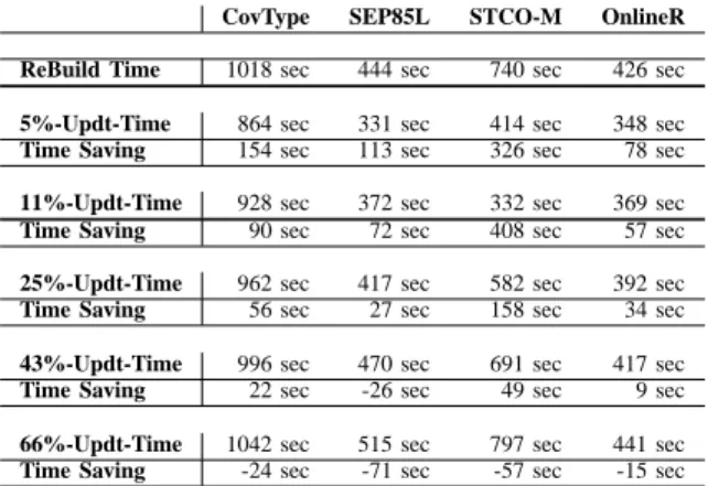
Table IX represents the time saved by incremental update, in comparison with the time to rebuild entirely the last-half data cube of the updated fact table. In Table IX,
– Rebuild Time is the time for rebuilding entirely the last-half data cube of the updated fact table,
– x%-Updt-Time is the time for incremental update of the last-half data cube where x% is the ratio of the size of the
second part to the size of the first part and,
– Time Saving is the difference between Rebuild Time and
x%-Updt-Time.
All the times includes the computation time and the in-put/output time, in seconds. Table IX shows that when the ratio of the size of the new fact table to the size of the current fact table varies from 5% to 25%, the incremental update is more
interesting. Afterward, it would be better to rebuild entirely the last-half data cube of the updated fact table.
VIII. CONCLUSION ANDFURTHER WORK
This work is an extension of [1] that represents a data cube by its last-half: the set of cuboids called prime (or next-prime) cuboids. All other cuboids are computed by a simple operation, called the aggregate-projection, based the last-half data cube. The representation is reduced because only a half of the data cube is stored using the binary search prefix tree (BSPT) structure. Such a structure offers not only a compact representation but also an efficient search method. Building a cuboid in the last-half data cube is reduced to building a BSPT. The BSPT allows efficient group-by operation without previous sort operation on tuples in the fact table or in cuboids.
TABLE IX. TIME SAVING BY DATA CUBE UPDATE
CovType SEP85L STCO-M OnlineR ReBuild Time 1018 sec 444 sec 740 sec 426 sec
5%-Updt-Time 864 sec 331 sec 414 sec 348 sec
Time Saving 154 sec 113 sec 326 sec 78 sec
11%-Updt-Time 928 sec 372 sec 332 sec 369 sec
Time Saving 90 sec 72 sec 408 sec 57 sec
25%-Updt-Time 962 sec 417 sec 582 sec 392 sec
Time Saving 56 sec 27 sec 158 sec 34 sec
43%-Updt-Time 996 sec 470 sec 691 sec 417 sec
Time Saving 22 sec -26 sec 49 sec 9 sec
66%-Updt-Time 1042 sec 515 sec 797 sec 441 sec
Time Saving -24 sec -71 sec -57 sec -15 sec
Each cuboid in the representation is in fact an index table in which tuples have a list of RowIds referencing to tuples in the fact table. The experimental results show that the average time for computing the a cuboid with the aggregate functions COUNT and SUM based on this representation is among the average time of the efficient methods. Moreover, based on this representation, we can compute the cuboids for any aggregate function and any measure, without rebuilding the representation when we change the measure or the aggregate function.
The experimental results of the incremental update on the four real datasets, using the Direct method, show that the time saving, with respect to the Reconstruction method, is interesting when the ratio of the size of the new fact table to the size of the current fact table varies from5% to 25%. When the
ratio is greater than40%, it would be better to rebuild entirely
the last-half data cube of the updated fact table.
On the above experimental results, we can conclude that the approach is interesting not only in computing time, storage space, and representation, but also interesting for querying and incremental update. As we can efficiently access to all aggregated tuples in the data cube, it is interesting to study the application of this representation in data mining, in particular, for classification or detection of anomalies.
REFERENCES
[1] V. Phan-Luong, “A Simple and Efficient Method for Computing Data Cubes,” in Proceedings of the 4th International Conference on Communi-cations, Computation, Networks and Technologies (INNOV), November 15-20, 2015, Barcelona, Spain, pp. 50-55.
[2] S. Agarwal et al., “On the computation of multidimensional aggregates,” in Proceedings of the 22nd International Conference on Very Large Data Bases (VLDB), 1996, Mumbai (Bombay), India, pp. 506-521. [3] V. Harinarayan, A. Rajaraman, and J. Ullman, “Implementing data cubes
efficiently,” in Proceedings of the 1996 ACM SIGMOD, Montreal, Canada, pp. 205-216.
[4] S. Chaudhuri and U. Dayal, “An Overview of Data Warehousing and OLAP Technology,” SIGMOD Record Vol. 26, Issue 1, 1997, pp. 65-74. [5] Y. Zhao, P. Deshpande, and J. F. Naughton, “An array-based algorithm for simultaneous multidimensional aggregates,” in Proceedings of the 1997 ACM SIGMOD International Conference on Management of Data, Tucson, Arizona, USA, pp. 159-170.
[6] J. S. Vitter, M. Wang, and B. R. Iyer, “Data cube approximation and histograms via wavelets,” in Proceedings of the 7th International Conference on Information and Knowledge Management (CIKM), 1998, Bethesda, Maryland, USA, pp. 96-104.
[7] K. S. Beyer, R. Ramakrishnan, “Bottom-up computation of sparse and iceberg cubes,” in Proceedings of the 5th ACM International Workshop on Data Warehousing and OLAP, (SIGMOD), 1999, Philadelphia, Penn-sylvania, USA, pp. 359-370.
[8] J. Han, J. Pei, G. Dong, and K. Wang, “Efficient Computation of Iceberg Cubes with Complex Measures,” in Proceedings of the 2001 ACM SIGMOD International Conference on Management of Data, Santa Barbara, California, USA, pp. 1-12.
[9] D. Xin, J. Han, X. Li, and B. W. Wah, “Star-cubing: computing iceberg cubes by top-down and bottom-up integration,” in Proceedings of the 29th International Conference on Very Large Data Bases (VLDB), 2003, Berlin, Germany, pp. 476-487.
[10] Z. Shao, J. Han, and D. Xin, “Mm-cubing: computing iceberg cubes by factorizing the lattice space”, in Proceedings of the International Con-ference on Scientific and Statistical Database Management (SSDBM), 2004, pp. 213-222.
[11] Y. Sismanis, A. Deligiannakis, N. Roussopoulos, and Y. Kotidis, “Dwarf: shrinking the petacube,” Proceedings of the 2002 ACM SIG-MOD International Conference on Management of Data, Madison, Wisconsin, pp. 464-475.
[12] Y. Sismanis and N. Roussopoulos, “The polynomial complexity of fully materialized coalesced cubes,” in Proceedings of the 30th International Conference on Very Large Data Bases (VLDB), 2004, Toronto, Canada, pp. 540-551.
[13] L. Lakshmanan, J. Pei, and J. Han, “Quotient cube: How to summarize the semantics of a data cube,” in Proceedings of the 28th International Conference on Very Large Data Bases (VLDB), 2002, Hong Kong, China, pp. 778-789.
[14] L. Lakshmanan, J. Pei, and Y. Zhao, “QC-Trees: An Efficient Summary Structure for Semantic OLAP,” Proceedings of the 2003 ACM SIGMOD International Conference on Management of Data, pp. 64-75.
[15] A. Casali, R. Cicchetti, and L. Lakhal, “Extracting semantics from data cubes using cube transversals and closures,” in Proceedings of the 9th ACM SIGKDD International Conference on Knowledge Discovery and Data Mining (KDD), 2003, Washington, D.C., pp. 69-78.
[16] A. Casali, S. Nedjar, R. Cicchetti, L. Lakhal, and N. Novelli, “Lossless Reduction of Datacubes using Partitions,” International Journal of Data Warehousing and Mining (IJDWM), 2009, Vol. 5, Issue 1, pp. 18-35. [17] W. Wang, H. Lu, J. Feng, and J. X. Yu, “Condensed cube: an efficient
approach to reducing data cube size,” in Proceedings of the International Conference on Data Engineering (ICDE), 2002, pp. 155-165.
[18] Y. Feng, D. Agrawal, A. E. Abbadi, and A. Metwally, “Range cube: efficient cube computation by exploiting data correlation,” in Proceedings of the International Conference on Data Engineering (ICDE), 2004, pp. 658-670.
[19] K. A. Ross and D. Srivastava, “Fast computation of sparse data cubes,” in Proceedings of the 23rd International Conference on Very Large Data Bases (VLDB), 1997, pp. 116-125.
[20] K. Morfonios and Y. Ioannidis, “Supporting the Data Cube Lifecycle: The Power of ROLAP,” The VLDB Journal, July 2008, Vol. 17, No. 4, Springer-Verlag New York, Inc., pp. 729-764.
[21] J. Gray et al., “Data Cube: A Relational Aggregation Operator Gen-eralizing Group-by, Cross-Tab, and Sub-Totals,” in Data Mining and Knowledge Discovery, 1997, Vol. 1, Issue 1, pp. 29-53, Kluwer Academic Publishers, The Netherlands.
[22] J. A. Blackard, “The forest covertype dataset,” ftp://ftp. ics.uci. edu/ pub/machine-learning-databases/covtype, [retrieved: April, 2015]. [23] C. Hahn, S. Warren, and J. London, “Edited synoptic cloud re- ports
from ships and land stations over the globe,” http://cdiac.esd.ornl.gov/ cdiac/ndps/ndp026b.html, [retrieved: April, 2015].
[24] “2010 Census Modified Race Data Summary File for Counties Alabama through Missouri,” http://www.census.gov/popest/research/ modified/STCO-MR2010 AL MO.csv, [retrieved: September, 2016]. [25] “Online Retail Data Set,” UCI Machine Learning Repository,
https://archive.ics.uci.edu/ml/datasets/Online+Retail, [retrieved: Septem-ber, 2016].
[26] D. Chen, S. Liang Sain, and K. Guo, “Data mining for the online retail industry: A case study of RFM model-based customer segmentation using data mining,” Journal of Database Marketing and Customer Strategy Management, 2012, Vol. 19, No. 3, pp. 197-208.
![Table III presents the experimental results approximately got from the graphs in [20], where “avg QRT” denotes the average query response time and “Construction time” denotes the time to construct the (condensed) data cube](https://thumb-eu.123doks.com/thumbv2/123doknet/14579343.728974/9.918.510.821.124.357/presents-experimental-results-approximately-response-construction-construct-condensed.webp)