HAL Id: hal-00777464
https://hal.inria.fr/hal-00777464
Submitted on 17 Jan 2013HAL is a multi-disciplinary open access archive for the deposit and dissemination of sci-entific research documents, whether they are pub-lished or not. The documents may come from
L’archive ouverte pluridisciplinaire HAL, est destinée au dépôt et à la diffusion de documents scientifiques de niveau recherche, publiés ou non, émanant des établissements d’enseignement et de
Fast L_1-C
kpolynomial spline interpolation algorithm
with shape-preserving properties
Eric Nyiri, Olivier Gibaru, Philippe Auquiert
To cite this version:
Eric Nyiri, Olivier Gibaru, Philippe Auquiert. Fast L_1-Ckpolynomial spline interpolation algorithm
with shape-preserving properties. Computer Aided Geometric Design, Elsevier, 2011, 28 (1), pp.65-74. �10.1016/j.cagd.2010.10.002�. �hal-00777464�
Fast
L
1− C
kpolynomial spline interpolation
algorithm with shape-preserving properties
Eric Nyiri
1,
Olivier Gibaru
1,2,
Philippe Auquiert
11 Arts et Metiers ParisTech, L2MA, 8 Boulevard Louis XIV, 59046 Lille Cedex 2 INRIA Lille-Nord-Europe, 40, avenue Halley 59650 Villeneuve d’Ascq, France
Abstract
In this article, we address the interpolation problem of data points per regular L1
-spline polynomial curve that is invariant under a rotation of the data. We iteratively apply a minimization method on five data, belonging to a sliding window, in order to obtain this interpolating curve. We even show in the Ck-continuous interpolation
case that this local minimization method preserves well the linear parts of the data, while a global Lp (p ≥ 1) minimization method does not in general satisfy this
property. In addition, the complexity of the calculations of the unknown derivatives is a linear function of the length of the data whatever the order of smoothness of the curve.
Key words: L1 spline, interpolation, shape preserving, smooth spline
Introduction
In geometric modelling, a common requirement is that the computational curves ‘preserve shape’, which means the curves express the geometric prop-erties of the interpolated data in accordance with human perception. These geometric properties are variously interpreted as linearity, monotonicity, con-vexity and smoothness. Conventional splines, which are calculated by mini-mizing the square of the L2 norm of the second partial derivatives of a cubic
piecewise polynomial interpolant, represent sufficiently ”smooth” data quite well. However, they often have extraneous, nonphysical oscillations when used for interpolation of data with abrupt changes.
Recently, a new kind of splines called cubic L1 splines has arisen (Cf. [5], [6],
[7], [9], [15], [17]). Cubic L1 splines, which are calculated by minimizing the
L1 norm of the second derivatives of a C1-smooth piecewise cubic interpolant,
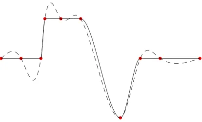
Fig. 1. L2 (dotted line) versus L1(solid line) global interpolations
we show that the univariate interpolating cubic L1 spline of a set of points
lying over a Heaviside function entirely agrees with the function (i.e the two half lines) except at the jump.
Although many different interpretations of shape preservation can be found in literature (Cf. [13], [23], [24]), there is no widely accepted quantitative de-scription of shape preservation. In the present paper, we accept the observation made by most observers that L1 splines preserve shape well as justification for
working on improving the algorithm to calculate L1 splines and the shape
preserving properties (Cf Fig. 1).
The L1 spline is issued from the minimization of a nonlinear functional. Since
nonlinear programming procedures for minimizing the L1 spline functional are
not yet practical for global data interpolation, a discretization of this func-tional is commonly used. Minimization of the discretized L1 spline functional
which is a nonsmooth convex programming problem, leads to solving of an overdetermined linear system that can be reduced to a linear program for which many methods are available. In literature, a compressed primal affine method has been the most common choice. This method is based on the pri-mal affine algorithm by Vanderbei, Meketon and Freedman (Cf. [27], [28], [25], [26]) and it is described in [16]. The primal-dual algorithm [17,20,24,28] is widely considered to be the most efficient and robust interior-point method.
We introduce a local minimization method based on a sliding window defined over five points so as to interpolate data points smoothly. This local method allows us to define a fast computational algorithm issued from the algebraic calculus of the exact solution over five points only. Furthermore, we show that a five points window allows us to preserve the linear parts of the data points while in general the global method does not satisfy this property. Moreover, we show that if we apply this strategy iteratively we can define Ck-continuous
solutions also have shape-preserving properties.
This paper is organized as follows. In Section 1, we give some results concerning C1-continuous cubic L
1 spline interpolation on three and five points. Based on
these results, in Section 2 we define a new interpolation strategy with a sliding five points window to create a local L1C1 interpolating method. By applying
iteratively this method we are able to construct Ck-continuous interpolating
spline curves in IRd(with d ≥ 1). In Section 3, we demonstrate that the linear
parts of the data are preserved and we also give some other properties. Some conclusions will be drawn in the last section.
1 The C1−continuous cubic L
1 spline interpolation on five points
Let a = u1 < u2 <···< un = b be an arbitrary and strictly monotonic partition
of the finite real interval [a, b]. In [2], we deal with the parametric case where we wish to interpolate a set of data points P1, . . . , Pn belonging to IRd (with
d≥ 1). The ui are chosen according to the classical chordal partition (see [12]
Section 4.4.1 page 201). This choice seems to give the best results in most data configurations. The C1 interpolating cubic spline curve is calculated by
minimizing the L1−norm of the second derivative vector of the spline. If we
denote by ∆ the classical forward difference operator, we showed in [2] that the solution to this problem is obtained by minimizing the following functional
E(T1, . . . , Tn) = n−1 X i=1 Z 12 −1 2 k∆Ti+ 6t(Ti+1+ Ti− 2 ∆ui ∆Pi)k1dt (1)
where the Ti ∈ IRd are the first order derivative vectors at points Pi for
i = 1, . . . , n. As E(T1, . . . , Tn) is not strictly convex, then its minima are
not necessarily unique. To reduce the set of solutions, Lavery in [14] added a ‘regularization’term so as to select the derivative vectors Ti which are as short
as possible in the L1-norm. Consequently, a C1-continuous cubic L1 spline is
obtained by minimizing the following functional
E(T1, . . . , Tn) + ε n
X
i=1
|Ti|, (2)
where ε is a strictly positive real. As this problem is also nonlinear, this func-tional is discretized by using the midpoint rule method for each integral. the resulting problems raised by the L1-minimization of linear systems1 are solved
by the Vanderbei, Meketon and Freedman primal affine algorithm defined in [28] and outlined in [16].
From now on, we shall be interested in calculating the exact solutions to the minimization problem (1) when we have a set of five points. To do so first, we shall study the three-point case.
1.1 Univariate cubic L1C1 interpolation over three points
The following lemma gives the exact solution to the minimization of (1) with n= 3.
Lemma 1 Let (ui, zi)i=1,2,3 be three couples of real values where u1 < u2 < u3
and the slopes be defined by hi =
∆zi ∆ui for i = 1, 2. Let min (b2,b3)∈IR 2Φ(b1, b2, b3) (3) with Φ(b1, b2, b3) = Z 12 −1 2 |∆b1+6t(b2+b1−2h1)|dt+ Z 12 −1 2 |∆b2+6t(b3+b2−2h2)|dt, (4) be a univariate C1-continuous L
1 cubic spline interpolation minimization
prob-lem where b1, b2 and b3 are the first derivative values at the three points. The
solutions to (3) are a) if b1 is comprised between h1+ √ 10+1 3 (h2− h1) and h1 then b2 = h1+ √ 10−1 3 (b1− h1) , b3 = h2+ √ 10−5 5 (h1 − h2) + 5−2 √ 10 5 (b1− h1) ,
b) if b1 is comprised between h1 and h1+ √ 10−5 5 (h2− h1) then b2 = h1− 5+ √ 10 3 (b1 − h1) , b3 = h2+ √ 10−5 5 (h1− h2) + (b1− h1) , c) otherwise b2 = b3 = h2. (5)
PROOF. Function Φ(b1, b2, b3) is the sum of two positive convex continuous
functions. The minimal value 2(
√ 10−1)
3 |b2− h2| of the second integral
accord-ing to the variables (b2, b3) is obtained for b3− h2 = √
10−5
5 (b2− h2). By using
the following variables x = b1− h1 and y = b2− h1, we can infer from Lemma
4 of [3] that min (b2,b3)∈IR 2Φ(b1, b2, b3) = min y∈IR H(x, y) , (6)
where H(x, y) = 2(√10−1) 3 |y + h1− h2| + |y − x| if |y − x| ≥ 3 |x + y| , 2(√10−1) 3 |y + h1− h2| + 3 2|x + y| + (y − x)2 6 |x + y| else. (7)
If we consider the following function ϕh1,h2(x) = min
y∈IR
H(x, y), then after some calculations we obtain for any x ∈ IR that the minimal values are given for
y= min³h2− h1,min ³√ 10−1 3 x,− √ 10+5 3 x ´´ if h2− h1 <0, min³h2 − h1,max ³√ 10−1 3 x,− √ 10+5 3 x ´´ else. (8)
Case a) : If we assume that h2 − h1 < 0 then from (8) we infer that for
any b1 ∈ h h1+ √ 10+1 3 (h2 − h1) , h1 i , b2 = h1+ y = h1 + √ 10−1 3 (b1− h1) and b3 = h2+ √ 10−5 5 (b2− h2) = h2+ √ 10−5 5 (h2− h1) +5−2 √ 10 5 (b1− h1). The other
cases are obtained from (8) similarly. Then the solutions to (3) given by (5) are satisfying.
In the following subsection we shall calculate the subdifferential of the con-tinuous convex function ϕh1,h2(x) = min
y∈IR
H(x, y) defined in (6). Let us define the following functions :
ϕ1 h1,h2(x) = − 3 2(x + h2− h1) − (h2−h1−x)2 6(x+h2−h1), ϕ2 h1,h2(x) = 8−4√10 3 x+ 2(√10−1) 3 (h1− h2) , ϕ 3 h1,h2(x) = 2(√10−1) 3 (h1− h2) , ϕ4h1,h2(x) = ϕ1 h1,h2(x) , ϕ 5 h1,h2(x) = x − h2+ h1, ϕ 6 h1,h2(x) = −ϕ 1 h1,h2(x) .
Consequently according to (7) and (8), we can infer that
ϕh1,h2(x) = σϕ
k
h1,h2(x) if x ∈
h
min³σxkh−11,h2, σxkh1,h2´,max³σxkh−11,h2, σxkh1,h2´i, (9) where σ = {1 if h2− h1 ≥ 0 and − 1 otherwise} and
x0h1,h2 = −∞, x 1 h1,h2 = √ 10+1 3 (h2− h1) , x 2 h1,h2 = 0, x 3 h1,h2 = √ 10−5 5 (h2− h1) , x4h1,h2 = −1 2(h2− h1) , x 5 h1,h2 = −2 (h2− h1) , x 6 h1,h2 = +∞. (10)
1.2 Univariate cubic L1C1 interpolation over five points
From now on, we shall be interested in giving the solutions to the following univariate L1C1 interpolation problem on five points. Let (ui, zi)i=1,...,5 be
five couples of real values where u1 < · · · < u5 and the slopes be defined
by hi =
∆zi
∆ui
for i = 1, . . . , 5. Hence, the univariate L1C1 spline solution is
obtained from min (b1,...,b5)∈IR 5 4 X i=1 Z 12 −1 2 |∆bi+ 6t(bi+1+ bi− 2hi)|dt
where the bi are the derivative values of the spline at ui. This functional is the
sum of positive and convex continuous functions. It can be written by
min b3∈IR min (b2,b1)∈IR 2Φ(b3, b2, b1) + min (b4,b5)∈IR 2Φ(b3, b4, b5) (11) = min b3∈IR ϕh2,h1(b3− h2) + ϕh3,h4(b3− h3)
where Φ is defined by (4) in the previous lemma and ϕhi,hj by (9). Let us
denote by ∂ϕhi,hj(x) the subdifferential of ϕhi,hj(x) at x (Cf. [4],[11]). Since
(11) is convex and continuous its subdifferential is compact and nonempty.
Let us define dg(x) = min ∂ϕh2,h1(x − h2) + min ∂ϕh3,h4(x − h3) and dd(x) =
max ∂ϕh2,h1(x − h2)+max ∂ϕh3,h4(x − h3) respectively the left and right
deriva-tive values of (11) at x. We define a sorted list {βk}k=1...10 from the abscissa
³
xjh3,h4 + h3, xjh2,h1 + h2
´
j=1,...,5. As function (11) is convex the minimal value
is obtained for any b3 such that dg(b3).dd(b3) ≤ 0. Consequently b3 is between
α1 = min
k∈{1,...,10}(βk such that dg(βk)dd(βk) ≤ 0 or dd(βk)dg(βk+ 1) < 0) and
α2 = max
k∈{1,...,10}(βk such that dg(βk)dd(βk) ≤ 0 or dd(βk− 1)dg(βk) < 0). Three
cases can thus be identified:
(1) α1 = α2 : the solution is unique and b3 = α1 = α2.
(2) α1 6= α2, dd(α1) = 0 and dg(α2) = 0 : The solutions for b3 are [α1, α2]. In
this case we choose b3 = min x∈[α1,α2] ¯ ¯ ¯x− h2+h3 2 ¯ ¯
¯ so as to preserve linear parts
when possible.
(3) α1 6= α2, dd(α1) 6= 0 and dg(α2) 6= 0 : The value of b3 is unique and it
belongs to ]u1, u2[. We calculate this value by using a dichotomic search
algorithm.
2 Local cubic Lk
1Ck interpolation method
To define a Ck-continuous parametric spline curve with degree 2k + 1 which
interpolates a set of points (Pi)i=1,...,n, one must define the derivative vectors
up to the kth order at these points. We propose to calculate these
deriva-tive vectors by applying iteraderiva-tively for each coordinates the previous L1C1
interpolation algorithm within windows which contain only five data for each derivative order. In the following subsections we shall give more detail about this method.
2.1 Local cubic L1C1 interpolation method
From now on we shall consider the C1 case. We define a five-point sliding
window on a set of points and we calculate the derivative vector only for the middle point (Cf. Fig. 2). By translating the window, point by point over all the data, we obtain a derivative vector at each interpolation point. Hence, we are able to construct a cubic L1-spline.
Fig. 2. Sliding window over the sets of points
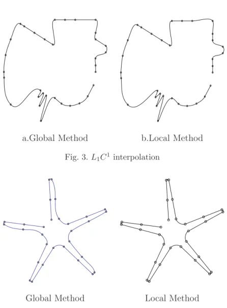
If we visually compare the results obtained by Lavery’s L1C1 global method
and our local one (see Figure 3), we can see that they are quite identical. The two parts which differ are a corner2 and a point at the bottom3.
Since the L1 minimization algorithm does not produce invariant curves with
respect to the rotation of the data, we proposed in [2] to get it by using a local change of coordinates for 2D data points. On each interval [ui, ui+1], we define
a coordinate system (Pi, −→ui, −→vi) such that Pi+1 coordinates in this system are
(k−−−−→Pi√Pi+1k
2 ,
k−−−−→Pi√Pi+1k
2 ). This method which has been developed for the global L1C 1
interpolation method is quite costly in computing time as the dimension of the matrix issued from the primal affine algorithm is multiplied by two and this local change of coordinates cannot easily be extended to d > 2 dimensional data. In our local algorithm, another reason why this change of coordinates cannot be used is that the functional to minimize thus obtained changed for each set of five points. Here, we simply propose to apply a local change of coordinates to the five points belonging to the sliding window before applying
2 where the minimization problem has a range of solutions for the derivative vectors 3 because the minimization functions are quiet different
a.Global Method b.Local Method
Fig. 3. L1C1 interpolation
Global Method Local Method
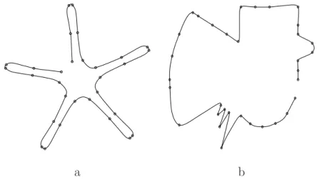
Fig. 4. Star L1C1 interpolation
the minimization method. Consequently, the invariance is satisfied and the method minimizes the functional (1) on this new frame. For instance with 3D data points, we define an orthonormal frame based on the points belonging to each sliding window . For any pair of sets of five points equivalent up to a rotation, this local change of coordinate method gives the same derivative vector up to the rotation for the middle point of the sets. As we only keep this middle value to construct the L1-spline solution, that result provides a
coherent shape on the curve.
2.2 Local Lk
1Ck interpolation method (k ≥ 2)
In [2], a global L1C2 method was given so as to construct a parametric quintic
the following function n−1 X i=1 1 ∆ui Z 1 2 −1 2 |αi(t) Ti+1+ βi(t) Ti+ γi(t) Mi+1+ δi(t) Mi+ ηi(t) ∆Pi|dt (12) + ǫ1 n X i=1 |Ti| + ǫ2 n X i=1 |Mi|
where the Mi are the second derivative vectors at points Pi, αi(t) = 32+ 15t −
6t2− 60t3, β i(t) = −32+ 15t + 6t2− 60t3, γi(t) = ³ −14 − 32t+ 3t2 + 10t3´∆u i, δi(t) = ³ −14 + 32t+ 3t2− 10t3´∆u i and ηi(t) = −30t+120t 3
∆ui . Here, ǫ1 and ǫ2 are
positive reals.
If we study the resulting curves thus obtained (See Fig. 5) we can see that they are smooth and do not oscillate too much.
a b
Fig. 5. Global L1C2 interpolation method
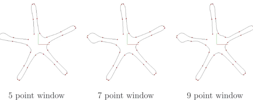
Therefore we have tested a sliding window method with the primal affine algorithm on the sets of points as in the L1C1 case. We thought that this
method could improve the result so that we could study the functional to minimize. On the contrary, the curves show more oscillations (See Fig. 6)
Nevertheless, we found that the local L1C1 interpolation method produces
good spline curvature results between the data points even if the spline curves are only C1continuous at the data points. Like Lavery in [20], we decided to use
the first derivative vectors obtained by our local L1C1 interpolation method,
but with another scope. In his article, Lavery calculated the first derivative vectors TCubic
i by minimizing (2) over (ui, Pi) and then he found the second
derivative vectors Mi minimizing (12) by using (ui, Pi, Ti = TiCubic). This
two-step procedure allows to reduce the complexity of the minimization calculus but it prevents using our previous studies over cubic splines. We propose a new
5 point window 7 point window 9 point window
Fig. 6. Local L1C2 interpolation method with windows changing size
C2 method, denoted by L2
1C2 which is obtained by applying twice the local
L1C1 interpolation method. We firstly apply it on the data points (ui, Pi) so
as to obtain the first derivative vectors Ti. We apply it again onto the (ui,Ti)
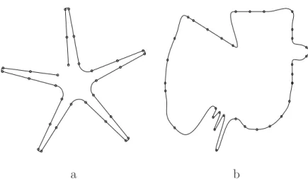
in order to calculate the second derivative vectors Mi. As we can see in Figure
7, the quintic spline curve solution has shape preserving properties. As we show further down, our Lk
1Ck method allows us to benefit from the ‘shape
preserving’property of the local L1C1 algorithm.
a b
Fig. 7. L21C2 interpolation method
This L2
1C2 sliding window method needs a nine-points sliding window.
Actu-ally, we need Pi−2, . . . , Pi+2 so as to calculate vector Ti and each vector Mi is
calculated from vectors Ti−2, . . . , Ti+2.
If we want to construct Ck-continuous splines (with k ≥ 2), we have to
cal-culate the derivative vectors up to the kth order. To do so, we can simply use
our local L1C1 method repeated k times, which is noted Lk1Ck for k ≥ 1
(con-sequently L1
1C1 = L1C1). As our local L1C1 algorithm has shape preserving
properties, we shall think that this iterative method will produce smooth high degree spline curves. As we can see in Figure 8, the curves are C3-continuous and they preserve the data well.
a b
Fig. 8. local L31C3 interpolation method
3 Properties of the local L1C1 algorithm
3.1 Linear shape preservation
For any arbitrary set of points, our local L1C1 produces linear curve parts
when up to three points lie on a line, contrary to the global L1C1 solution
curve (Cf. Fig. 9).
Fig. 9. Global L1C1 interpolation
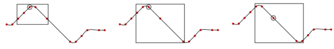
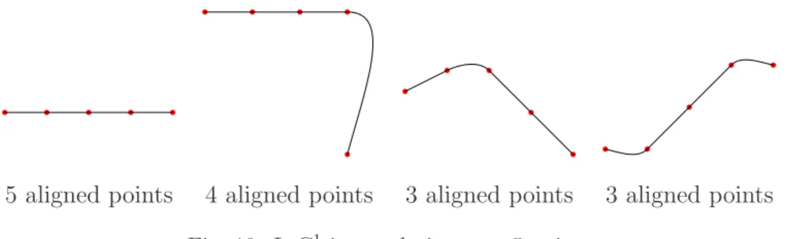
In the univariate case, we showed in [1] that for interpolation points belonging to the Heaviside function, where three of them are located on one of the half-line of this function, the derivative vectors at these points are necessarily collinear to this line. Actually, in the parametric case over some sets of five points, we can see in Figure 10 that the L1C1 cubic interpolation produces
derivative vectors which are collinear when three points lie on a line.
To demonstrate this property, we first study the univariate case. By using the fact that the ui are fixed according to the chordal parametrization, we then
5 aligned points 4 aligned points 3 aligned points 3 aligned points
Fig. 10. L1C1 interpolation over 5 points
show that linear parts are preserved in IRd (with d ≥ 1), which implies that the derivative vectors Ti at such points are collinear.
Lemma 2 Let (ui, αi)i=1,...,5 be five couples of real values where u1 < u2 <
· · · < u5. We denote by hi =
∆αi
∆ui
for i = 1, . . . , 4 the slopes between the points. The minimization problem
min (b1,...,b5)∈IR 5 4 X i=1 Ã Z 12 −1 2 |∆bi+ 6t(bi+1+ bi− 2hi)|dt ! (13)
has the following solutions :
a) if hi = hi+1 = h for i = 1 (resp. i = 3) except the case hj = hj+1 6= h for
j = 3 (resp. j = 1) then b3 = bi = bi+1 = h,
b) if h2 = h3 = h and (h1− h) (h4− h) < 0 then b1 = h1+h4+ √ 10−5 5 (h − h1) , b2 = b3 = b4 = h and b5 = h4+ √ 10−5 5 (h − h4) ,
c) if h2 = h3 = h and (h1− h) (h4− h) > 0 then b2 = b4 = h and b3 is
comprised between h and min³h+√10−55 (h4− h) , h + √
10−5
5 (h4− h)
´
,
d) if h1 = h2 and h3 = h4 with h1 6= h3 (we call it the corner case) then
b1 = b2 = h1, b4 = b5 = h3 and b3 is comprised between h1 and h3.
Moreover if we add ¯¯ ¯b3− h2+h3 2 ¯ ¯
¯ to (13) then the solution is unique in each
cases and b3 = h2+h2 3.
PROOF. From (11), we know that this minimization problem (13) can be written as follows :
min
b3∈IR
ϕ(b3) = ϕh2,h1(b3− h2) + ϕh3,h4(b3− h3)
where the ϕhi,hj are positive convex functions. Since hi = hi+1 = h (for i = 1 or
i= 3) then ϕhi,hi+1(b3− h) =
5
3|b3− h|. As the minimal value of this strictly
convex function at b3 = h is equal to zero, consequently whatever the values
of the other slopes (except for case d)), ϕ has a unique minimum at b3 = h.
Hence, property a) holds. Case d) : If h1 = h2 and h3 = h4 with h1 6= h3 then
ϕ(b3) = 53|b3− h1| + 53|b3− h3| is minimal for any b3 comprised between h1
comprised between h and h +√10−55 (h1− h). Similarly for ϕh3,h4(b3− h3) the
minimum value is obtained for b3 comprised between h and h+ √
10−5
5 (h4− h).
Moreover, their minimal values are equal. For (h1− h) (h4− h) > 0, these
in-tervals overlap. Hence, the minimum of ϕ is obtained for b3 comprised between
h and min³h+√10−55 (h4− h) , h + √ 10−5 5 (h4− h) ´ . If (h1− h) (h4− h) < 0
then the minimal value of ϕ is only obtained for b3 = h. Consequently, if we
add¯¯ ¯b3 − h2+h3 2 ¯ ¯
¯to the minimization function ϕ, then for each case, b3 =
h2+h3
2
is the unique solution.
The linear parts of the data can be preserved in each cases. For case d) there are two such solutions. The following proposition allows us to extend the previous univariate study to the parametric case.
Proposition 3 Let P1, P2,. . . ,P5 be five data points. We associate to each
point Pi a real value ui such that u1 < u2 < · · · < u5. The ui are chosen
according to the chordal partition. If at least three data points are aligned then
the minimization problem (1) has a unique interpolation L1C1 cubic spline
which preserves the linear part except in the corner problem where there are two such solutions.
PROOF. In this case, we have to minimize (1) with n = 5. As we use the L1-norm, this minimization can be done on each coordinate separately. In
ad-dition, the chordal partition allows us to keep the same value for the slope between each consecutive coordinate issued from aligned data points. Conse-quently, the result can therefore be inferred by using the previous proposition.
Similarly to the C1-continuous case, the L2
1C2 method gives quintic spline
with linear parts when the data points lie on a line. Actually, the first use of the local L1C1 algorithm always gives first derivative vectors which are
collinear with lines defined by the aligned data points. Hence, the second use of this algorithm on these vectors also gives collinear vectors. This property can be extended to Lk
1Ck interpolation methods which are simply obtained by
iterating this process.
3.2 Good curvature
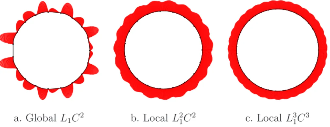
In Figure 11, we have created curves that interpolate twenty points which lie on a circle. As we can see, the local method gives good curvatures4 which are 4 the curvature of the spline is represented by an offset according to the curvature
almost monotonous contrary to the solution of the global L1C2 interpolation
case.
a. Global L1C2 b. Local L21C2 c. Local L31C3
Fig. 11. Curvatures for circle approximation by a ”closed” 20 points set
The splines obtained by local Lk
1Ck, k ≥ 2 method are relatively smooth
without oscillations (see. Figure 12). This is partly due to the fact that we have a smooth set of derivative vectors by applying many times our local L1C1
algorithm . We can see in Figure 12.c that the splines do not oscillate too much despite the high degree of the spline curves5.
a. Local L2 1C2
b. Local L3
1C3 c. Local L51C5
Fig. 12. Curvatures for a snail like data set interpolated by local Lk
1Ck methods
3.3 Computational complexity
In our local five-point window algorithm, the time needed to calculate each derivative vector is small and almost constant. Hence, the time needed to calculate the global spline curve is linear and we can interpolate large data sets of points. Moreover, our original iterative approach allows us to calculate Ck
continuous interpolation spline curves with a linear time complexity. Indeed, to create a Ck interpolation spline curve of degree 2k + 1, we need to apply
the local L1C1 method, which allows us to preserve this linear complexity, k
times consecutively on the successive data.
In addition to this, our local L1C1 algorithm can be parallelized on
multi-processor computers by distributing the computation of each five-point win-dow over the processors. That is possible as each calculus is independent at each stage. Furthermore, for the Ck continuous interpolating curves, the
itera-tive use of the local L1C1 method allows us to start the calculus of the first kth
derivative vector when five k −1th derivative vectors are known. Consequently,
we only need a sliding window of 4k + 1 points for a Ck spline. This allows us
to accelerate the calculus.
For example, to compute the local L2
1C2 quintic spline solution, we only need
a nine-point sliding window so as to be able to parallelize the calculus.
4 Conclusion
We have defined a local method which is efficient to interpolate sets of data points by univariate cubic splines using the L1 norm. This method keep the
shape-preserving properties without having the drawback of the commonly used global L1 method : Our method use algebraic results which are faster
and more stable than the numerical approximations used before. We can use it to calculate Ck-continuous curves with good curvature despite their high
degrees. Furthermore, it is very simple to parallelize the calculus. If we want to reduce the time spent on calculations on a very large number of data, we need a large number of processors. Because our methods can be used in IRd, the interpolation of data by spline curves from various domains (Cf. [8], [10]) is possible keeping the good properties of our algorithm. We currently use the L21C2 interpolation method for enhanced trajectory planning for machining with industrial six-axis robots (Cf. [22]).
5 Acknowledgments
The authors thank the referees for their helpful suggestions and comments.
References
[1] P. Auquiert, Interpolation de points par des splines L1 r´eguli`eres, Phd Thesis,
Universit´e de Valenciennes et du Hainaut-Cambr´esis, LAMAV, (20 d´ecembre 2007).
[2] P. Auquiert, O. Gibaru, E. Nyiri, C1 and C2-continuous polynomial parametric
Lp splines (p ≥ 1), Comp. Aided Geom. Design 24 (2007), 373–394.
[3] P. Auquiert, O. Gibaru, E. Nyiri, On the cubic L1 spline interpolant to the
Heaviside function, Numer. Algor. 46 (2007), 321–332.
[4] D. Az´e, El´ements d’analyse convexe et variationnelle, Ellipses, (1997).
[5] H. Cheng, S.-C. Fang, J.E. Lavery, Univariate cubic L1 splines—A geometric
programming approach, Math. Methods Oper. Res. 56 (2002) 197–229.
[6] H. Cheng, S.-C. Fang, J.E. Lavery, An efficient algorithm for generating univariate cubic L1 splines, Comput. Optim. Appl. 29 (2004) 219–253.
[7] H. Cheng, S.-C. Fang, J.E. Lavery, Shape-preserving properties of univariate cubic L1 splines, J. Comput. Appl. Math. 174 (2005) 361–382.
[8] O. Gibaru, Tensorial rational surfaces with base points via massic vectors. SIAM J. Numer. Anal. 42, n◦4 (2004), 1415-1434.
[9] D.E. Gilsinn, J.E. Lavery, Shape-preserving, multiscale fitting of bivariate data by cubic L1 smoothing splines, in: C.K. Chui, L.L. Schumaker,
J. St¨ockler (Eds.), Approximation Theory X:Wavelets, Splines, and Applications,Vanderbilt University Press, Nashville, TN, (2002), pp. 283–293. [10]L. Han, L.L. Schumaker, Fitting monotone surfaces to scattered data using C1
piecewise cubics, SIAM J. Numer. Anal. 34 (1997) 569–585.
[11]J.B. Hiriart-Urruty, C. Lemar´echal, Fundamentals of Convex Analysis, Springer, (2001).
[12]Hoschek, J., Lasser, D. Fundamentals of computer Aided Geometric Design, A.K. Peters, Wellesley, 1993.
[13]F. Kuijt, R. van Damme, Shape preserving interpolatory subdivision schemes for nonuniform data, J. Approx. Theory 114 (2002) 1–32.
[14]J.E. Lavery, Univariate cubic Lp splines and shape-preserving, multiscale
interpolation by univariate cubic L1 splines, Comput. Aided Geom. Design 17
[15]J.E. Lavery, Shape-preserving, multiscale fitting of univariate data by cubic L1 smoothing splines, Comput. Aided Geom. Design 17 (2000) 715–727.
[16]J.E. Lavery, Shape-preserving, multiscale interpolation by bi- and multivariate cubic L1 splines, Comput. Aided Geom. Design 18 (2001) 321–343.
[17]J.E. Lavery, The state of the art in shape preserving, multiscale modeling by L1 splines, in: M.L. Lucian, M. Neamtu (Eds.), Proceedings of SIAM Conference on Geometric Design Computing, Nashboro Press, Brentwood, TN, (2004), pp. 365–376.
[18]J.E. Lavery H. Cheng, S.-C. Fang, Shape-preserving properties of univariate cubic L1 splines, Journal of Computational and Applied Mathemetics 174
(2005), 361–382.
[19]J.E. Lavery, Shape-preserving, first-derivative-based parametric and non parametric cubic L1 spline curves, Comput. Aided Geom. Design 23 (2006),
276–296.
[20]J.E. Lavery, Shape-preserving univariate cubic and higher-degree L1 splines
with function-value-based and multistep minimization principles, Computer Aided Geom. Design 26 (2009), 1–16.
[21]I.J. Lustig, R.E. Marsten, D.F. Shanno, Interior point methods for linear programming: computational state of the art, ORSA J. Comput. 6 (1994) 1–14. [22]A. Olabi, R. Bare, E. Nyiri, O. Gibaru, L1paramatric interpolation and feedrate
planing for machining robots, The Swedish Production Symposium G¨oteborg, Sweden, (2-3 december 2009)
[23]J. Peters, Smoothness, fairness and the need for better multisided patches, in: R. Goldman, R. Krasauskas (Eds.), Topics in Algebraic Geometry and Geometric Modeling, Contemporary Mathematics, vol. 334, American Mathematical Society, Providence, RI, (2003), pp. 55–64.
[24]F.I. Utreras, The variational approach to shape preservation, in: P.J. Laurent, A. Le Mehaut´e, L.L. Schumaker (Eds.), Curves and Surfaces, Academic Press, NewYork, 1991, pp. 461–476.
[25]R.J. Vanderbei, Affine-scaling for linear programs with free variables, Math. Program. 43 (1989) 31–44.
[26]R.J. Vanderbei, LOQO: An interior point code for quadratic programming, Statistics and Operations Research Technical Report SOR-94-15, Princeton University, (1995).
[27]R.J. Vanderbei, Linear Programming: Foundations and Extensions, second ed., Kluwer Academic, Boston, (2001).
[28]R.J.Vanderbei, M.J. Meketon, B.A. Freedman,A modification of Karmarkar’s linear programming algorithm, Algorithmica 1 (1986) 395–407.
[29]Y.Wang, S.-C. Fang, J.E. Lavery, H. Cheng, A geometric programming approach for bivariate cubic L1 splines, Comp. Math. Appl. 49 (2005) 481–514. [30]Y. Wanga, S.-C.Fang, J.E. Lavery, A compressed primal-dual method for generating bivariate cubic L1 splines, Journal of Computational and Applied Mathematics 201 (2007) 69–87.