HAL Id: inria-00070334
https://hal.inria.fr/inria-00070334
Submitted on 19 May 2006
HAL is a multi-disciplinary open access
archive for the deposit and dissemination of
sci-entific research documents, whether they are
pub-L’archive ouverte pluridisciplinaire HAL, est
destinée au dépôt et à la diffusion de documents
scientifiques de niveau recherche, publiés ou non,
computational grids
Eddy Caron, Frédéric Desprez, Cédric Tedeschi
To cite this version:
Eddy Caron, Frédéric Desprez, Cédric Tedeschi. Service discovery in a peer-to-peer environment for
computational grids. RR-5679, INRIA. 2005, pp.30. �inria-00070334�
ISRN INRIA/RR--5679--FR+ENG
a p p o r t
d e r e c h e r c h e
Thème NUM
Service discovery in a peer-to-peer environment for
computational grids
Eddy Caron — Frédéric Desprez — Cédric Tedeschi
N° 5679
computational grids
Eddy Caron , Fr´
ed´
eric Desprez , C´
edric Tedeschi
Th`eme NUM — Syst`emes num´eriques Projet GRAAL
Rapport de recherche n 5679 — September 2005 —30pages
Abstract: Les grilles de calcul sont des syst`emes distribu´es dont l’objectif est l’agr´egation et le partage de ressources h´et´erog`enes g´eographiquement r´eparties pour le calcul haute performance. Les services d’une grille sont l’ensemble des applicatifs que des serveurs met-tent `a disposition des clients. Une probl´ematique largement soulev´ee par les utilisateurs de grilles est la d´ecouverte de services. Les m´ecanismes actuels de d´ecouverte de services manquent de fonctionnalit´es et deviennent inefficaces dans des environnements dynamiques `a large ´echelle. Il est donc indispensable de proposer de nouveaux outils pour de tels envi-ronnements. Les technologies pair-`a-pair ´emergentes fournissent des algorithmes permettant une d´ecentralisation totale de la construction et de la maintenance de syst`emes distribu´es performants et tol´erants aux pannes. Le probl`eme que l’on cherche `a r´esoudre est de perme-ttre une d´ecouverte flexible (recherche multicrit`eres, compl´etion automatique) des services dans des grilles prenant place dans un environnement dynamique `a large ´echelle (pair-`a-pair) en tenant compte de la topologie du r´eseau physique sous-jacent.
Key-words: grid computing, peer-to-peer technology, service discovery
This text is also available as a research report of the Laboratoire de l’Informatique du Parall´elisme http://www.ens-lyon.fr/LIP.
pair-`
a-pair pour les grilles de calcul
R´esum´e : Grid computing is a form of distributed computing aiming at aggregating avail-able geographically distributed heterogeneous resources for high performace computing. The services of a grid is the set of software components made available by servers to clients. Ser-vice discovery is today broadly considered by grid’ users as inefficient on large scale dynamic platforms. Today’s tools of service discovery does not reach several requirements: flexibility of the discovery, efficiency on wide-area dynamic platforms. Therefore, it becomes crucial to propose new tools coping with such platforms. Emerging peer-to-peer technologies provide algorithms allowing the distribution and the search of files taking into account the dynam-icity of the underlying network. This report present a new tool merging grid computing and peer-to-peer technologies for an efficient and flexible service discovery in a dynamic and large scale environment, taking into account the topology of the underlying network. Mots-cl´es : grilles de calcul, technologies pair-`a-pair, d´ecouverte de services
1
Introduction
Over the last decade, grids connecting geographically distributed resources (computing re-sources, data storage, instruments, etc.) have become a promising infrastructure for solving large problems. However, several factors (scheduling, security, etc) still hinder its worldwide adoption. Among them, one is currently broadly regarded as a significant barrier to large scale deployment of such grids: service discovery.
The services of a grid is the set of software components made available on it. Through the history of grid computing, several mechanisms have been proposed and adopted. Those traditional approaches, efficient in a static and small scale environment where resources are clearly identified (most of the time in a centralized manner), lose their effectiveness on peer-to-peer platforms, i.e., in dynamic, heterogeneous large scale environment, where future grids shall inexorably take place.
Emerging peer-to-peer technologies allow the search of resources in dynamic large scale environments. Distributed Hash Tables (DHTs) [10,11, 14,20] are structured peer-to-peer technologies providing scalable distribution and location of resources by name-based routing. However, DHTs present two major drawbacks. First, they are logically built, thus breaking the physical topology of the underlying network resulting in poor routing performances. Second, they offer only rigid mechanisms of retrieval, allowing the search of resources only by their name. As we shall see in Section 2, several works are currently done in these two areas.
Iamnitchi and Foster have suggested in [9] that grids, that provide the infrastructure for sharing resources, but do not fit the dynamic nature of today’s large scale platforms, would take advantage of adopting peer-to-peer tools. To date, very few grid platforms have implemented Peer-to-Peer technologies.
1.1
Problem definition and components
Different approaches exist for building computational grids. We consider services pre-installed on servers and clients that discover them in order to remotely execute the service with their own data. A service will be described by several attributes, like its name, the processor type or the operating system of the server providing it. The theoretical problem we address in this paper is fivefold:
1. Multicriteria search. Grid’s users wish to discover services by any of the attributes of the service.
2. automatic completion. For instance, a user may want to discover all the services of the SUN S3L library, whose every routine’s name begins with the “S3L” string. 3. Uniform distribution of the work load. The tool must uniformly distribute the
work load on physical nodes in order to be scalable.
4. Fault-tolerance. The tool must take into account the dynamic nature of the under-lying network, i.e., dynamic joins and leaves of nodes.
5. Quick responsiveness. Clients are impatient to receive servers references to be able to remotely execute their computation.
1.2
Contribution
First, in Section 2, this paper give a brief overview of the state of the art in peer-to-peer technologies providing flexible discovery mechanisms and topology aware DHTs. After hav-ing described how we model services in Section3, the contribution of this paper is introduced in Section 4: the Distributed Lexical Placement Table (DLPT). The DLPT is a novel ar-chitecture using a peer-to-peer approach based on a lexical tree (trie) of each attribute for a flexible service discovery providing automatic completion and multicriteria search. The DLPT uniformly distributes the load on the nodes of the physical network (the peers) while addressing the dynamic nature of the underlying network by adopting a replication mech-anism. It also addresses the locality issue by finding a spanning tree of the graph of the different logical routes built by replication and provides cache optimizations for quick re-sponsiveness. Then, in section7, we give an analysis of our architecture, and simulation in section8. Finally, we give a conclusion and our future work.
2
Related work
2.1
DHT
Distributed Hash Tables [10,11,14,20] are attractive solutions to distribute work load and storage in a dynamic network. Resources are referenced as a (key, value) pair. They provide uniform distribution of work load on the nodes, each node being responsible of the storage of the same number of keys. They ensure the routing consistency by providing mechanisms of detection and prevention of nodes’ departures. Replication prevents from loosing resources. Because of those advantages we first studied DHT for the service discovery on the grid, each server declaring its services by a (key, value) pair (typically, (name, location)) to the DHT and clients submitting requests on a given key. However, DHTs do not address sev-eral of our requirements. DHTs allow to retrieve resources by only one attribute, used to generate the key. Another solution is then to store services according to all their attributes, but the automatic completion is still impossible. In addition, as we already pointed out, logical connection of the DHT breaks the topology of the physical network, resulting in poor performance routing, what contradict our requirement of quick responsiveness. The two following subsections summarize recent work addressing these drawbacks.
2.2
Topology aware DHT
Many works have been undertaken to build topology aware DHTs, i.e., to make logical links reflecting the physical topology, to make physical neighbors logical neighbors. Different appraoches have been studied, but the most promising way to introduce the physical topology in DHT-like networks is to build hierarchies of DHTs.
Hierarchical DHTs
In the Hierarchical DHT issue, we consider relevant to distinguish two approaches:
Supernodes Brocade [19] is made of two levels of DHTs. The key idea of the supernodes is to allow each local domain to manage its own DHT, and to elect one or several supernodes among the nodes of this DHT, considering their CPU power, bandwidth and proximity with a backbone, fanout. . . The supernodes of each local DHTs form a kind of super-DHT, connecting each local DHT by high-speed links. This concept has been generalized to any levels [4], has been adapted to the IP numbering [6]. In [16], each node, at its insertion time, determine itself if it’s a supernode (considering globally known criteria) and choose its own neighbors. Jelly [8] proposes an architecture in which a joining node inserts the domain whose supernode minimizes latency with itself or became itself supernode.
Landmarks Another approach, introduced by the authors of CAN [10] consists in using a set of nodes, the landmarks, distributed on the physical network, that is used to dispatch nodes in bins considering a given metric, typically the latency. For instance, let us consider m landmarks. m! orderings are possible, m! logical bins are created, each node being placed in the bin corresponding to the ordering he get by testing its latency with each landmark and ordering them. The underlying assumption is that nodes close to each other in the physical network will have close ordering and thus belong to close bins. Ecan [18] adopt the same approach but build a hierarchy of bins, grouping for instance two close bins at level 1 in the same bin of level 2. HIERAS [17] adopt an hybrid aproach between landmark and supernodes. At last, the authors of [16] identify each node with its ordering on the landmarks, thus giving the position of a node in a m-dimension Cartesian space, and then reducing this space to a 1-dimension space using the space filling curves that preserves locality achieving this transformation.
The hierarchical DHTs call upon network management tools (autonomous systems, local administrative domains, IP numbering) and make the assumptions that local connections are always quicker than long distance connections. As we already seen it, landmarks based approaches make the assumptions that you have a globally known set of nodes reflecting the underlying network, what seems to be difficult to implement in a dynamic network. Among these mechanisms, only Jelly doesn’t rely on such unrealistic assumptions.
2.3
Flexible Discovery in DHT
The other major drawback of using DHT is their rigid mechanisms of retrieval, allowing retrieving resources only by one key. A series of work, initiated by Harren et al. [7] and still in progress, aim at addressing the issue of allowing DHT to provide more complex mechanisms of discovery.
Semistructured description of resources
First achievements in this way have been the ability to retrieve resources described by an unstructured language. In INS/Twine [2], each resource is described by an XML file. Start-ing from this description, one can determine the set of potential requests concernStart-ing one or several attribute in this description. Each request is then represented by a unique character string, from which a key can be generated and placed on the DHT. Recently,Biersack et al [5] have adopted a similar approach but distributing the resolution of the request among several nodes.
[1, 13] propose to request the DHT on a set of numerical values, [15] extend classical database operations to DHT. But our closest related work is the SQUID project.
The Squid project
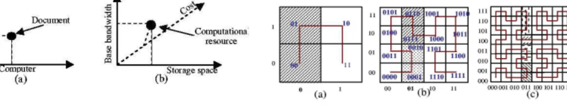
Based on [1], the Squid project [12] is the most advanced merging work between service discovery and DHT-based network, since they propose a totally distributed architecture for the web service discovery, traditionally based on a centralized server, and providing automatic completion of requests and multicriteria search. Each service is described by a fixed number of keywords. Thus, each service can be represented as a point in the multi-dimensional keyword space, as illustrated on figure 1. The discovery is made on a set of keywords, partial keywords and jokers. For instance, for services described by three keywords, a discovery request sent by the client is (matrices, comp*, *)
Figure 1: Spaces of dimensions 2 and 3. Document is described by keywords Net-work and Computer.
Figure 2: Recursive refinements of the Hilbert space filling curve
Each point in the coordinate space receive a unique identifier by using the Hilbert space filling curve, as illustrated on figure2for binary 2-digits keywords. For instance, the service defined by the combination (11, 01) get the identifier 1100 (we follow the curve starting from the (00, 00) point that receiver the identifier 0 and increment the identifier at each step. As we already pointed out, space filling curve provide the property to preserve locality. Thus, close points in the multi-dimensional cube get close identifiers. Those identifiers are mapped on an underlying DHT thus receiving the services’ description.
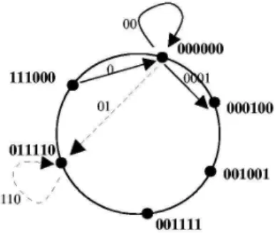
The mechanism of processing the discovery request (011, *) is illustrated on figure 2. The authors exploit the recursive nature of space filling curves and distribute the requests among the nodes of the underlying DHT at each step of refinement. A cluster define a set of sub-cubes, from which the curve enter and leave only once. Each cluster receive an identifier composed of the digits shared by all points of this cluster. The rest of the identifier is then padded with zeros. The refinement of this cluster is then executed by the node whose identifier is the closest of the cluster’s identifier among the DHT’s nodes. For instance, at step (b), the hatched cluster contains two sub-cubes whose identifiers are 0110 and 0111. Consequently, this cluster receive the identifier 011000. The request for refining this cluster is consequently sent to the node of the DHT whose identifier is closest to 011000, let us assume 011110. The refinement of this cluster will give birth to two sub-clusters (c). The recursive refinement is viewed as a tree on figure3and generated messages on the DHT are shown on figure4. When the identifier of the request is greater than the required identifier, all services corresponding to the request are on this node and the request is stopped.
Despite significant advances brought by the Squid project, it has several drawbacks: 1. Services are not uniformly distributed in the keyword space, resulting in a non uniform
work load distribution on the nodes.
2. Squid is layered on top of a DHT. Each generated message result in a number of logical hop logarithmic in the number of nodes. Thus, in the worst case, for a request of type (*, *, *) if the network size is N , the number of message required will be N log(N ), each node being contacted.
3. The number of dimensions is statically set at the beginning of the system, forcing users to describe and looking for services with this number of keywords. Moreover, a discovery request must contain the required number of dimensions, and if not will be padded with jokers, resulting in a useless cost when processing the request.
4. Squid doesn’t address the locality problem.
Those aspects of Squid are major drawbacks hindering us to reach our requirements. That’s why we decided to propose our own architecture, allowing a flexible and fast efficient service discovery on the grid, involving quite simple mechanisms, but outperforming classical DHT and the Squid project regarding complexities and functionalities, as we shall see in the next section.
3
Modeling services
In the following of this paper, we consider that services are described by a set of attributes. Grids’ users traditionally want to discover services by following attributes:
1. The name of the services The name of the service is the name under which the software component searched is known. For instance, DGEMM, DTRSM (from the BLAS library [3]), S3L mat mullt addto (from the SUN S3L library).
Figure 3: Requests tree
Figure 4: Messages generated on the DHT
2. The processor type of the server The coding of data changes according to the processor type. It is useful to know it to avoid users to send miscoded data and loose precious time. For instances, Power PC, x86, etc.
3. The operating system of the server In the same way, the various operating sys-tems do not have the same characteristics and functionnalities, what can induce per-formances variations. For instances, Linux Mandrake, MAC OS 9, etc.
4. The complete location of the peer For locality considerations between the client and the server or because the users trusts a given cluster, a client can specify a machine or a cluster of machines on which he wishes his data to be processed. To ease the auto-matic completion, we consider the specification of machine/cluster/network in reverse notation when considering the full name of the machine. For instance, fr.grid5000.*, edu.*, etc. the location could be specified with its IP address, too.
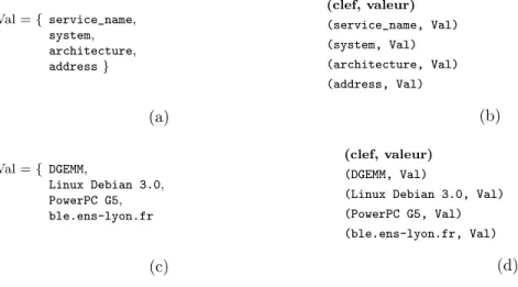
This model is illustrated in the figure5. The value of services is composed at most of all these attributes, and at least of one of them (a). To allow storing and retrieving the services considering one or several attributes, a (key, value) pair is created for each attribute (b). The service is thus stored according to each key in the DLPT.
4
The Distributed Lexical Placement Table: general
de-scription
In this section, we make a general description of the contribution of this paper, the Dis-tributed Lexical Placement Table, storing references of services in a reduced lexical tree (reduced trie) whose logical nodes are distributed among physical nodes.
DLPT functionalities The DLPT stores object references (here, services declared by servers) with (key, value) pairs. The DLPT retrieves values corresponding to a key,
Val = { service_name, system, architecture, address} (a) (clef, valeur) (service_name, Val) (system, Val) (architecture, Val) (address, Val) (b) Val = { DGEMM, Linux Debian 3.0, PowerPC G5, ble.ens-lyon.fr (c) (clef, valeur) (DGEMM, Val)
(Linux Debian 3.0, Val) (PowerPC G5, Val) (ble.ens-lyon.fr, Val)
(d)
Figure 5: Services and colrresponding (key, value) pairs
when processing a discovery request sent by a client. The DLPT provides automatic completion of discovery requests on partial keys. For instance, let us assume services are described by their name, a client sending the request (DT R∗) will receive all services whose name begins with (DT R), for instance DT RSM , DT RM M . The DLPT do not rely on a hashing function but relies on a lexical placement algorithm. Logical architecture. The DLPT relies on a reduced lexical tree (whose unary nodes have been suppressed). The basic entity of this tree is the logical node. Each logical node stores services referenced by one key. A key can be of two types: A real key is the key corresponding to at least one value, i.e., one service effectively declared by a server. For instance, DGEMM is a real key as soon as a server has declared a service under the DGEMM name. Note that by construction, every leaf of the tree store real keys. A virtual key represents the set of keys, real or virtual, that share a same prefix. More formally, let n be a node storing a virtual key whose identifier, i.e., the key it stores, is id(n). n is also the root of the subtree whose nodes’ identifier are prefixed by id(n). Figure6 shows the construction of such a tree.
Mapping the logical tree on the physical network The logical nodes of the tree are distributed on the physical nodes of the underlying network. Let’s call them peers. A logical node is hosted by a peer. A peer has the ability to host zero, one or more logical nodes, each logical node being a process running on it.
Routing complexity. Whereas logical nodes of DHTs represent physical nodes, logical nodes of the DLPT represent keys of declared services. Thus, the tree grows
according to the number of distinct keys declared. We wil see in Section 7 that the routing complexity of the DLPT is independent of the network size.
Dynamicity and failure. The DLPT, like DHTs, is designed to take place in a dynamic environment. It provides a mechanism of replication of the nodes and links of the tree, in order to remain efficient facing the departure of peers.
Uniform distribution of the load and minimization of the communication time We first want to distribute the load by uniformly distribute the logical nodes on the peers. Then, among the possible routes generated by the replication process, we choose to periodically determine a minimum spanning tree. We use a greedy heuristic for this purpose.
Figure 6: Construction of a tree considering the name as attribute of the services, by declar-ing “DGEMM”, “DTRSM” and “DTRMM” services. Nodes stordeclar-ing a real key are black filled circle. The node storing real keys “DTRSM” and “DGEMM” share the same prefix “D” (2), the node storing real key “DTRMM” and node storing virtual key “D” share the empty string, identifier of the root of the tree.
5
Creation and maintenance of the DLPT
It is important to note that services are declared in a dynamic manner. We do not a priori know how will the tree be like, he dynamically evolves according to services begin declared.
5.1
Dynamic construction of the lexical tree
We now consider the insertion of one (key, value) pair. The pair is placed inside the lexical tree according to the key. Like in a DHT, the peer declaring a service gets the address of a peer hosting a logical node of the tree by an out-of-band mechanism (name server, web
page, ...) and sends an insertion request to it. The request is routed in the tree until reaching the node that will insert the pair. Each node, on receipt of an insertion request on the S = (key = k, value = v) pair applies the following routing algorithm, considering four distinct cases:
k is equal to the local node identifier. In this case, k is already in the tree, no node need to be added, the logical node inserts v into its table.
k is prefixed by the local node identifier. The local node looks among its children identifiers sharing one more character than itself with k. If such a child exists, the request is forwarded to it, else, no node identifier in the tree prefix k with more char-acters than the local node identifier. A new logical node is created as a child of the local node, v is inserted in the table of the new node.
The local node identifier is prefixed by k. In this case, if the identifier of the parent of the local node is equal to or prefixed by k too, S must be inserted upper in the tree and the local node forwards the request to its parent. Otherwise, S must be inserted in this branch, between the local node and its parent. Such a logical node is created that inserts v into its table.
No relation of equality or prefixing. If the local node has a parent and the identifier of the parent of the local node is equal to or is prefixed by the common prefix to k and the local node identifier, the local node forwards the request to it. Otherwise, the logical node storing k and the logical node are siblings. However, their common parent does not exist. Two nodes must be created, the node storing k (sibling of the local node) and their parent whose identifier is the common prefix to k and the local node identifier (possibly the empty string).
5.2
Dynamic mapping of the logical nodes onto the physical
net-work
We now discuss how the mapping of logical nodes onto peers. One of our requirements is to uniformly distribute the load among the peers. When designing the DLPT, we made the assumption that each logical node has an equivalent load, as supposed in most DHTs. On one hand, the amount of requests that will traverse a logical node is inversely proportional to this node depth. On the other hand, storing a real key, whose probability is proportional to the node depth, results in processing request and communicating with clients. These two antagonist aspects led us to consider the load equivalent on every logical node. A finer theoretical study is needed, but we believe it is here out-of-topic. We now describe two architectures we have defined to implement the DLPT in a real environment.
Centralized approach In a first architecture shown in Figure7, the mapping relies on a central device. Obviously, this device is only used for the mapping and does not have any role when processing insertion or discovery requests. The peers, when connecting
the network, joins the DLPT by registering themselves to this central device. When a new logical node is created, a peer is uniformly-randomly chosen among the peers that registered to the central directory, to host it. This approach is intuitive, easy to implement, but as in every centralized systems, the central device is a central point of failure. Even if a solution could be to duplicate this device, this architecture is not fully distributed. This led us to define a distributed architecture.
Distributed approach In a second approach, each logical node is hosted by a peer on the underlying network, itself structured by a DHT, as illustrated on Figure 8. In the following, we consider this DHT is Chord [14], but any DHT could be used. Each logical node identifier id, will be placed according to the Chord mechanism, i.e., on the successor of H(id) on the Chord ring, where H is a uniform random hash function.
Figure 7: Partially centralized map-ping approach.
Figure 8: Fully distributed mapping approach.
5.3
Fault-tolerance
The DLPT takes place in a dynamic network in which nodes connect and disconnect without informing the network beforehand. This induces potential loss of links and/or nodes of the lexical tree.
To allow the routing process to remain efficient, as the nodes join and leave the network, we propose to duplicate logical nodes and links. Let k be the replication factor. k represents the number of distinct peers on which each logical node must be present. Such a replicated tree is shown in Figure9 Duplicating the nodes results obviously in duplicating the input and output links of this node and the table of values corresponding to the key stored. In order to ensure the uniform distribution of nodes on peers, the peers are randomly chosen in the central directory, when using the centralized approach. If using the totally distributed approach, we need k uniform random collision-resistant hash functions when k ≤ N selecting all peers when k > N , N being the number of available peers. This replication will be executed by a periodic algorithm, which role is to check that each nodes are available on k distinct peers.
Figure 9: Example of a replicated tree.
We consider k statically fixed at the beginning of the system. Another solution, allowing the dynamic setting of k, as the dynamicity level of the network changes, is being formulated.
5.4
Adaptation to the physical network heterogeneous performance
In order to fulfill our quick responsiveness requirement, we choose to minimize the communi-cation time in the replicated tree, by choosing the best link among the several identical links generated by the replication process. We thus need to determine a spanning tree minimiz-ing the communication time. Note that this spannminimiz-ing tree is not a classical one, generated by a distributed spanning tree algorithm. Each link having a semantic, one instance of each link must be kept in this spanning tree. Still considering the tree topology, each node has knowledge only about its parent (eventually replicated) and also its children (eventually replicated). Thus, the only possible minimization is a local one. So we use a greedy heuristic locally choosing the best link among the replicas of each distinct logical node. This heuristic is integrated to the replication process, without modifying its complexity, as we shall see in section7. During the process, when a node has replicated one child, it sends a message to each of the replicas of this child and choose the one minimizing the communication time. Until the next replication process, this one will be the recipient of the requests for this logical
child. This replica is also designated as responsible node of the replication of this child’s children.
5.5
Distributed algorithms of insertion and replication
We have described the DLPT in a general way. Let us now describe the distributed algorithm needed to implement such a system.
5.5.1 Messages
The processes must communicate together. We define now the set of messages and primitives used by the protocol.
The SEND(type, dest, data) primitive send a message of type type to the destination dest. The getPeer() primitive allows to obtain the address of peers, either by the central device, or by using the k hashing functions inside the Chord ring. We consider 6 types of messages:
INSERT. This message is an insertion request. It is sent from a server declaring a service, and then from each intermediate node en route for insertion.
CREATE.Sent by a peer creating a new logical node to the peer that will host it. INFO.This message is a request to inform other logical nodes that a creation happened. For instance, the node n creates a new logical node as its child. The replicas of n must be informed that they have a new child, but n does not know its own replicas. It sends a INFO message to its parent who knows all the replicas of n and can inform them. UPDATE.Sent by a peer on receipt of an INFO message. It informs the right nodes with the information needed to update their routing table, i.e., the list of their children and parent. For instance, on receipt of an INFO message, the parent whose one child has a new child send UPDATE messages to every replicas of this child to inform of their new child.
HEARTBEAT.This message is first sent by the root of the tree to initiate the replication process. On receipt of this message, a node applies the replication to children that do not reach the required number of replicas. It then selects the best replica according the communication time and designates it as the responsible node of the replication of the children of the logical node it hosts by sending him a HEARTBEAT message. REPLICATE. During the replication process, this type of message is sent by a node to a child who does not reach the replication factor. This type of message is sent with the list of peers on which the child must replicate (the data parameter). On receipt of this message, a node sends CREATION messages to these peers and an UPDATE message to all replicas of its parent and children so that they update their routing table with the new replicas.
5.5.2 Insertion
The distributed insertion algorithm is given by the pseudo-code of the algorithm 1. This algorithm starts the algorithm2
5.5.3 Replication and adaptation to the physical network
The replication process, described by the algorithm3is periodically initiated by the root of the tree, which starts by replicating itself if necessary. The root is the only one node that has knowledge about its replicas. The root’s replicas shape a full connected network. Each root is a potential starter of the replication process. First, it tests the number of its replicas, let k0 be this number. It replicates k − k0 times itself on peers it discovers via the central device or the underlying DHT, according to the chosen approach. It then sends a CREATE message with its own logical node structure to each of the peers previously discovered. Once the root is replicated, it sends a HEARTBEAT message to itself initiating the traversal of the tree.
On receipt of a HEARTBEAT message, a node processes as described in the algorithm 4. For each logical distinct child node, the node tests the number of reachable replicas and get the references of peers needed to reach k replicas (by sending a CREATE message to one of the current replicas. Finally, for each logical child node, it tests the communication time with each replica and sends a HEARTBEAT message to that which minimizes the communication time with itself.
Figure10illustrates the replication process, starting from a configuration where no repli-cation has been launched (1). Let us assume the replirepli-cation factor is k = 2. One replica is needed for the root and it requests one peer reference and sends its own logical node struc-ture to it. The root of the tree is the root of the spanning tree (2). The process continues through the tree. For each of its children, the root replicates the logical node considering the replication factor and designates that which minimizes the communication time with itself as the responsible node for the replication of their own children (3). In an asynchronous way, each selected replica launches the replication in its subtree, until reaching the leaves of the tree (4).
6
Interrogating the DLPT
We now describe the mechanisms allowing the service discovery according to a key or a set of keys.
6.1
Request on a full key
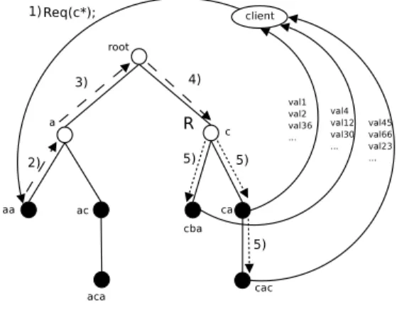
To process a discovery request according to a key, i.e., the traditional lookup(key) of DHTs, the DLPT executes the algorithm illustrated in Figure 11. The request is sent to a given node of the tree by the client, is routed in a way similar to that of an insertion request (see Subsection5.1) The destination node is the one that stores the key requested by the client,
Input:
Pair to insert S (key, value); Local Node ln;
begin
if key = ln.id then
ln.ST ORE(S); // Storing S in the table else if key prefixed by ln.id then
if ∃f ∈ ln.f ils, key pref ixed by f.id then
SEND(“INSERT”, f.addr[0], O); // Forwarding request to f else
Pair p ← GET P EER();
New Node n; // Creating a child
n.id← key; n.parentId ← ln.id; n.parentAddr[0] ← addrLocal; n.ST ORE(S);
SEND(“CREATE”, p, n); // requesting the hosting for a new child SEND(“INFO”, ln.parentAddr[0], n); // Inform my replicas end
else if ln.id prefixed by key then
if ((ln.parentId = c) or (ln.parentId prefixed by key)) then
SEND(“INSERT”, ln.parentAddr[0], S); // Forwarding request to my parent else
Peer p = GET P EER(); si ln.parentId =⊥ alors
// If no parent
New Node n; // a new root n.Id ← key; n.IN SERT (S); n.parentAddr←⊥;
n.ADDCHILD(n.Id, replicas); // The root knows itsd own replicas SEND(“CREATE”, p, n);
sinon
New Node n; // Creating an intermediate node between me and my parent n.Id← key;
n.ADDCHILD(n.id, addrLocal);
n.parentAddr← ln.parentAddr; n.parentId ← ln.parentId; n.ST ORE(O);
SEND(“CREATE”,p, n);
SEND(“INFO”, ln.parentAddr, n, p); // Inform the replicas of my parent of their new child
ln.parentAddr[0] ← p; ln.parentId ← clef // Changing my parent fin
end else
if ((ln.parentId = COM M ON P REF IX(key, ln.id)) or (ln.parentId prefixed by COM M ON P REF IX(key, ln.id))) then
SEND(“INSERT”, ln.parentAddr[0], O); else
Peer pf ← GET P EER(); Peer pp ← GET P EER();
New Node nf , np; // Creating sibling node and common parent node nf.id← key;
np.id← COM M ON P REF IX(key, ln.id);
np.ADDCHILD(ln.id, addrLocal); np.ADDCHILD(nf.id, pf ); np.parentAddr← ln.parentAddrAdr; np.parentId ← np.parentId; nf.parentAddr[0] ← pp; nf.parentId ← np.id;
SEND(“CREATE”, pf , nf ); SEND(“CREATE”, pp, np);
SEND(“INFO”, ln.parentAddr, np, pp); // Inform my parent’s replicas of their new child
ln.parentAddr[0] ← pp; ln.parentId ← COM M ON P REF IX(clef, ln.id); // Changing my parent
Input: Local node ln; New node n;
Peer hosting the new node p begin
// I am the parent of n if n.parentId = ln.id then
f← ln.GET CON CERN EDCHILD(n.id); // Inform n of the replicas of its children
SEND(“UPDATE”, n.addr, ln.childAddr[f ], ln.childId[f ]); // Updating my child ln.childId[f ] ← n.Id ln.childAddr[f ] ← p else
// I am the grandparent of n
f← ln.GET CON CERN EDCHILD(n.id);
// Inform each replica of this node’s parent of its new child (my grandkid) for i = 0 → ln.GET CON CERN EDCHILD(n.id).GET N BREP LICAS() do
SEND(“UPDATE”, ln.childAddr[f ][i], n); end
end end
Algorithm 2: Pseudo-code of the distributed algorithm launched on receipt of the INFO message.
Input: Local node ln; begin
nbReplicas ← GETNBREPLICAS(); // Determine the number of replicas of the root k0← nbReplicas − k; // k0missing replicas
si k0>0 alors
pour i = 0 → k0faire
Peer pi← GET P EER();
replicas[nbReplicas++] ← pi;
fin
for i = 0 → k0 do
SEND(“CREATE”, pi, ln, replicas);
end
pour i = 0 → ln.getN bChildren() faire
pour j = 0 → ln.child[i].GET N BREP LICAT S() faire SEND(“UPDATE”, ln.childAddr[i][j]);
fin fin fin
// Launching replication process to itself // Initiating tree traversal SEND(“HEARTBEAT”, addrLocal);
end
Algorithm 3: Pseudo-code of the periodic distributed algorithm of replication periodically launched on the root of the tree (REPLIC-SPANNING-TREE)
Input: Local node ln; begin
// For each distinct logical node child for i = 0 ← ln.GET N BCHILD() do // Determining number of replicas k0← ln.child[i].nbReplicas − k;
if k0>0 then
for j = 0 → k0− 1 do
Peer pi← GET P EER();
end
// Request the replication to one of the current existing replicas SEND(REPLICATE, ln.ChildAddr[i][j], p0, . . . , pk0−1);
end
PING REQ(); // Send a message of size of a request to know the replica minimizing the communication time with myself. The first peer answering is designated as responsible of the replication process in the subtree of this logical node. RECV (Ping response, p);
SEND(“HEARTBEAT”, p); end
end
Algorithm 4: Pseudo-code of the distributed algorithm of replication on receipt of a HEARTBEATmessage.
i.e., the node whose identifier is the requested key. Finally, the node storing the key wanted sends the corresponding values of services back to the client.
6.2
Request on a partial key
In order to achieve our automatic completion requirement, the DLPT processes requests on partial keys. The algorithm, made of two steps is illustrated on Figure12.
1. We first consider the explicit part of c, denoted exp(c). exp(c) is c without the joker part. For instance, exp(DT R∗) = DT R. The request is routed according to exp(c), in a similar way as for a fully explicit key, except that the destination node is the node whose identifier is the smallest key prefixed by exp(c). Let us call this node the responsible node for the request. The requested keys are in the subtree whose root is this responsible.
2. Once the responsible node has been found, one has to traverse every nodes of this subtree. We adopt an asynchronous traversal. As soon as a node of the subtree is reached, it sends back its values back to the client. The client has the opportunity to stop the reception of the responses, if he is satisfied with the values it received.
6.3
Cache optimizations
Figure 10: Replication process and spanning tree
6.3.1 Cache on partial keys
When processing a request on a partial key, the traversal of the subtree hosting requested keys is as expensive as the subtree is big. By caching values of the subtree during the traversal on the root of the subtree, we avoid clients to wait a long time by sending to it cached values as soon as the request reached the responsible node. Values are cached on processing the request. This mechanism is efficient as we assume that a requested key, will be eventually requested again.
6.3.2 Cache on full keys and popular keys
Popular keys will result in bottlenecks on peers hosting nodes storing popular keys. To avoid them to appear, we disseminate popular keys on several peers. When processing a request, the values retrieved on the node storing the requested key will be cached on peers hosting nodes on the route taken by the request to reach the destination node, by reverse routing. Thus, the most popular is a key, the most distributed will be its corresponding values. If a
Figure 11: Processing a discovery request (full key). The client sends the request to a node it knows (1). The request is routed (2,3,4).The node storing the requested key sends the corresponding values back to the client (5).
Figure 12: Processing of a discovery re-quest (partial key). The client sends the request to a node it knows (1). The request is routed to the responsible node accord-ing to the explicit part of the partial key (2,3,4). Asynchronous traversal and send-ing of responses (5).
request reach a peer caching values corresponding to a requested key, the routing ends and a response is immediately sent to the client, distributing the work load.
6.4
Multicriteria discovery
6.4.1 Insertion
Finally, we present mechanisms allowing the multicriteria retrieval. Remind that, as ex-plained in Section 3, a service is modeled by several attributes and will be placed in the DLPT according to each of them. However, placing values according to several attributes (for instance “DTRMM” and “linux”in the same tree will result in undesired behavior. For instance, if a machine has the name of a service, one will discover machines instead of ser-vices. To be sure of the nature of the information retrieved, we propose to build one tree per kind of attribute. Considering our model described in Section3, we dynamically build four trees, as services are declared. Let us consider again the example of Figure 5. The value of the service V al will be stored by sending an insertion request for each attribute to
a node the server knows for each tree. Thus, V al will be stored and retrieved considering each attribute.
6.4.2 Interrogation
To perform an interrogation on d0 criteria, where 1 ≤ d0 ≤ d, d being the number of trees/kind of attributes the system manages, the client must launch d0 requests to a node it knows in each of the trees containing the requested attributes. For instance, as illustrated on Figure13, to discover services fitting attributes’ value {DTRSM, Linux*, PowerPC*, *}, one will send three requests (the location of the machine has here no importance). The request on “DTRSM” will be sent to the services’ names tree, “Linux*” to the system tree and “PowerPC” to the processors tree. Requests are independently processed by each tree and the client asynchronously receives the values and finally just needs to intersect these values to keep what really match its interrogation.
7
Analysis of the DLPT
We place ourselves in the general case. Let a be a reduced lexical tree of size N (number of logical nodes) whose depth is d containing keys generated by an alphabet A. The maximum fanout of nodes is f .
7.1
Routing complexity
Theorem 1. The number of logical hops performed to route a request is independent of the size of the logical network (the tree) and is bound by twice the maximum size of the keys. Proof. We assume the generated keys have a size (number of characters) bound by T , thus d ≤ T . The number of logical children nodes of a node is at most f = Card(A). Thus, during its routing, in the worst case (from a node of depth T to another), a request will perform at most 2T logical hops.
Note that this upper bound is reached as soon as N = 2T +1, a having only two branches whose leafs are of depth T . In this case, the number of logical hops is in O(N ). Then, as the tree grows, the complexity remains the same, until a is f -balanced of depth d, what is the biggest tree that with keys generated by A. The number of nodes is now fd+1−1
d−1 = O(f d) and thus the number of logical hops 2T = 2d = O(log(N )).
7.2
Routing table size
Theorem 2. The routing table size is independent of the size of the logical network (the tree) size is bounded by Card(A).
Proof. The routing table of each node is composed of references to the children of this node. The maximum number of children for one node is Card(A) (At max one child by character of A).
We can note that this upper limit as soon as N = Card(A) + 1, a containing one node parent of all the other nodes (whose identifiers are all prefixed by the identifier of the first node). In this case, the routing table size is in O(n). Then, as the tree grows, the routing table size remains the same until the tree size reaches its maximum. The routing table size is also Card(A) = f = O(√N).
7.3
Local decision of routing
Theorem 3. The complexity of the local decision of routing is of O(1).
Proof. As we just pointed out, the maximum size of the routing table is Card(A), A be-ing globally known. In practice, Card(A) will be relatively small, for instance 65 (upper-case/lowercase characters). On each node, a vector of 65 address can thus be statically allocated. Consequently, to make the local decision of routing, only one test is needed.
7.4
Replication and spanning tree algorithm complexity
Theorem 4. The complexity of the replication process with determination of a spanning tree is linear in the size of the logical network (the tree) using the centralized approach to obtain peers’ references.
Proof. Considering a non replicated tree, the number of messages generated for the local replication of a node n (using the centralized approach to obtain peers’ references can be computed as follows, k being the replication factor):
1. Obtaining peers’ references 2 2. Determining the best replica 2k
3. Requesting the replication 1
4. Requesting the creation of n’s replicas k − 1 5. Informing the children of n ≤ Card(A) 6. Finding responsible node of the subtree replication 1
Finally, the complexity of the replication process is of O(k + Card(A)) for one node. For N nodes, i.e., for the whole tree, the complexity is thus O(N ∗ (k + Card(A))) = O(N) as Card(A) and k are constants. In a very similar way, we can show that this complexity is respected in a replicated tree.
Theorem 5. The complexity of the replication process with determination of a spanning tree is of O(N ∗ log(N)), N being the size of the logical network (the tree) using the distributed approach to obtain peers’ references.
Proof. The proof is very similar to the previous. The only difference is that using the distributed approach, the number of messages needed to obtain peer’s references is no more constant, but logarithmic (depending on the underlying DHT used).
7.5
Comparing the DLPT and DHTs
Table1summarizes the complexities of DHTs and those we just established of the DLPT for equivalent functionalities, i.e., requests on full keys (the only one type of requests a DHTs can process).
metric Chord CAN Pastry/Tapestry DLPT
Routing length O(log(N )) O(log(N )) O(log(N )) O(T ) Routing table size O(log(N )) O(log(N )) O(log(N )) O(Card(A)) Routing decision O(log(N )) O(log(N )) O(1) O(1)
Functionalities SQUID Multi-TPLD
Multicriteria discovery X X
Automatic completion X X
Variable number of criteria - X
Caching optimizations - X
Adaptation to the physical network - X Table 2: DLPT and Squid
Whereas DHTs have logarithmic routing length and logarithmic routing table size, the DLPT’s ones are independent of the network size. In addition, only the Pastry/Tapestry DHTs and the DLPT provide a number of tests to take the local routing decision in O(1).
7.6
Comparing the DLPT and Squid
Table 2 summarizes several aspects of both architectures and what are the advantages of the DLPT on Squid.
As we already pointed out in Section2.3, Squid [12] provides a static number of criteria, and every services must adopt this number, resulting in performance loss at time of discovery. The DLPT, by building a trie for each attribute, provides more flexibility and user’s facilities. As we shall see in Section8, the cache mechanisms inspired by the lexical nature of the DLPT provide an important improvement of the response latency. Finally, whereas Squid provides no mechanism of adaptation to the physical heterogeneous underlying network, the DLPT dynamically chooses links considering their performance. Note that to flood the entire logical network, O(N log(N )) messages are needed in the Squid approach and only O(N ) using the DLPT.
8
Simulation
A simulator of the lexical tree has been developed in Java. The dynamic creation of the tree and its interrogation with full and partial keys has been implemented, as well as their inherent caching mechanisms. It has been tested with typical computational grids data sets: 735 names of services, 129 names of processors, 189 OS names and 3985 names or IPs of machines. The random distribution used is the uniform one.
8.1
Building the tree and insertion requests
We first validated the logical algorithm of insertion of a newly declared service. Figure 14
represents the evolution of the size of the lexical tree according to the number of insertion requests submitted to the tree, with randomly picked keys. On the left, this evolution is given for the four data sets. As expected, as soon as all keys have been stored, the tree
does not grow anymore, all following insertion requests declaring already picked keys. On the right, we provide the same result but divided by the number of requests. In the same way, this fraction tends towards 0. On this experimental result a data set has been added made of generated keys of 1 to 20 characters themselves randomly picked among the Latin alphabet. This curve does not tend towards 0, since the probability of pick a key already in the tree is very small (only 20000 picks for this experiment and 2621
−1
25 ≈ 2 · 10 28
keys). In this case, the tree size remains proportional to the number of insertion requests processed. (up to 1.5 times the number of requests.)
0 1000 2000 3000 4000 5000 6000 7000 8000 0 5000 10000 15000 20000 tree size
Number of insertion requests 735 services (1006 nodes) [average]
189 OS (255 nodes) [average] 129 processors (173 nodes) [average] 3985 machines (5250 nodes) [average]
0 0.5 1 1.5 2 0 5000 10000 15000 20000
tree size/ number of insertion request
Number of insertion request 735 services (1006 nodes) [average]
189 OS (255 nodes) [average] 129 processeurs (173 nodes) [average] 3885 machines (5250 nodes) [average] Random words up to 20 characters [average]
Figure 14: Evolution of the tree size according to the number of insertion requests.
Then we have tested the number of logical hops when processing an insertion request. Figure15shows on the left the number of logical hops if all the requests enter the tree by its root. This gives an estimated average depth of the tree (approximately 4 for the four real data sets). On the right, Figure15shows the number of logical hops to process the request by choosing a random contact node. The behavior is close to those described in the analysis in Section 7: the curve quickly reaches an average depth and then follows a logarithmic behavior.
We have also studied how the tree grows according to the number of distinct declared keys. Each key is now inserted only once. As we see on Figure16, the total number of nodes in the tree (nodes storing virtual keys and nodes storing real keys) is proportional to the inserted keys (real keys). Sizes of the trees are summarized in the Table 3. In average, the proportion of nodes storing virtual keys is 30% with a standard deviation of 2.4%.
8.2
Interrogation requests and cache
Then we have studied the number of logical hops on the submission of interrogation requests. The results illustrated on Figure17are similar to those observed on insertion requests.
Finally, we studied the gain involved by the caching mechanism avoiding the bottlenecks on nodes storing popular keys. Figure 18 shows the number of logical hops for a set of
0 2 4 6 8 10 0 2000 4000 6000 8000 10000
Number of logical hops for an insertion
Number of insertion requests 735 services (1006 nodes) [average]
189 OS (255 nopeuds) [average] Random words up to 20 characters [average] 129 processors (173 nodes) [average] 3985 machines (5250 nodes) [average]
0 2 4 6 8 10 12 0 2000 4000 6000 8000 10000
Number of logical hops for an insertion request
Number of insertion requests 735 services (1006 nodes) [average]
189 OS (255 nopeuds) [average] Random words up to 20 characters [average] 129 processors (173 nodes) [average] 3985 machines (5250 nodes) [average]
Figure 15: Average number of logical hops (from the root, on the left, and from a randomly picked contact node among tree nodes, on the right).
- Services Systems Processors Machines
Number of real keys 735 189 129 3985
Number of nodes of the tree 1006 255 173 5250 Percentage of virtual keys 29,32% 34,38% 30.93% 27,94%
Table 3: Percentage of virtual keys for each data set.
0 200 400 600 800 1000 1200 0 100 200 300 400 500 600 700 Tree size
Number of real keys 735 services (1006 nodes) [average]
0 50 100 150 200 0 20 40 60 80 100 120 Tree size
Number of real keys 129 processors (173 nodes) [average]
Figure 16: Proportionality between the tree size and the number of real keys.
randomly-picked keys among keys stored in the tree with and without the caching mecha-nism. The number of logical hops decreases after a few random requests. Even with a little cache size (here, 50 values) the number of logical hops to find values corresponding to the requested key decreases significantly, going approximatively from 8 to 5.
0 2 4 6 8 10 0 200 400 600 800 1000
Number of logical hops for an interrogation request
Tree size
735 services (1006 nodes) [average]
0 2 4 6 8 10 0 1000 2000 3000 4000 5000
Number of logical hops for an interrogation request
Tree size
3985 machines (5243 nodes) [moyenne]
Figure 17: Number of logical hops for interrogation requests on full keys, according to the tree size. 0 2 4 6 8 10 12 0 2000 4000 6000 8000 10000
Number of logical hops for an interrogation request
Number of requests
735 services (1006 nodes) without caching [average] 735 services (1006 nodes) with caching [average]
Figure 18: Number of logical hops for an interrogation request on full keys with and without caching mechanism.
9
conclusion
After summarizing the state of art of the peer-to-peer technology, this report describes a novel tool, merging computational grids and a peer-to-peer approach to enhance an effi-cient, user oriented service discovery on large scale computational grids. This tool shows complexities that are equivalent or better than classical DHT approach and is. This tool is, to our knowledge the first to provide the automatic completion and multicriteria search
of services taking into account the heterogeneity of the physical underlying network links, and also efficient caching mechanisms allowed by the lexical nature of our system. Our five requirements described in section1.1have been addressed. This work is far to be over. First we made the assumption that every nodes in the tree receives the same work load, beacuse, as we explained it, it’s very hard to determine a priori this load. It would be interesting to model this load in order to obtain theoretical results about it. In a real environment, logs could help tuning this architecture.
References
[1] A. Andrzejak and Z. Xu. Scalable, efficient range queries for grid information services. In Peer-to-Peer Computing, pages 33–40, 2002.
[2] M. Balazinska, H. Balakrishnan, and D. Karger. INS/Twine: A Scalable Peer-to-Peer Architecture for Intentional Resource Discovery. In Proceedings of Pervasive 2002, 2002. [3] J. J. Dongarra, J. Du Croz, S. Hammarling, and I. S. Duff. A set of level 3 basic linear
algebra subprograms. ACM Trans. Math. Softw., 16(1):1–17, 1990.
[4] L. Garces-Erice, E. W. Biersack, K. W. Ross, P. A. Felber, and G. Urvoy-Keller. Hier-archical peer-to-peer systems. Parallel Processing Letters (PPL), 13(4), 2003.
[5] L. Garces-Erice, P. A Felber, K. W Ross, and G. Urvoy-Keller. Data indexing in peer-to-peer DHT networks. In ICDCS 2004, Tokyo, Japan, Mar 2004.
[6] L. Garces-Erice, K. W Ross, E. W Biersack, P. A Felber, and G. Urvoy-Keller. Topology-centric look-up service. In NGC’03, Munich, Germany, Sep 2003.
[7] M. Harren, J. Hellerstein, R. Huebsch, B. Loo, S. Shenker, and I. Stoica. Complex queries in dht-based peer-to-peer networks, 2002.
[8] R. Hsiao and S. De Wang. Jelly: A dynamic hierarchical p2p overlay network with load balance and locality. In ICDCS Workshops, pages 534–540, 2004.
[9] A. Iamnitchi, I. Foster, and D. Nurmi. A peer-to-peer approach to resource discovery in grid environments, 2002.
[10] S. Ratnasamy, P. Francis, M. Handley, R. Karp, and S. Shenker. A Scalable Content-Adressable Network. In ACM SIGCOMM, 2001.
[11] A. Rowstron and P. Druschel. Pastry: Scalable, distributed object location and routing for large-scale peer-to-peer systems. In International Conference on Distributed Systems Platforms (Middleware), November 2001.
[12] C. Schmidt and M. Parashar. Enabling flexible queries with guarantees in p2p systems. IEEE Internet Computing, 8(3):19–26, 2004.
[13] D. Spence and T. Harris. Xenosearch: Distributed resource discovery in the xenoserver open platform. In HPDC, pages 216–225, 2003.
[14] I. Stoica, R. Morris, D. Karger, M. Kaashoek, and H. Balakrishnan. Chord: A Scalable Peer-to-Peer Lookup service for Internet Applications. In ACM SIGCOMM, pages 149–160, 2001.
[15] P. Triantafillou and T. Pitoura. Towards a unifying framework for complex query processing over structured peer-to-peer data networks. In DBISP2P, pages 169–183, 2003.
[16] Z. Xu, M. Mahalingam, and M. Karlsson. Turning heterogeneity into an advantage in overlay routing. In INFOCOM, 2003.
[17] Z. Xu, R. Min, and Y. Hu. Hieras: A dht based hierarchical p2p routing algorithm. In ICPP, pages 187–, 2003.
[18] Z. Xu and Z. Zhang. Building Low-Maintenance Expressways for P2P Systems. Tech-nical report, Hewlett-Packard Labs, April 2002.
[19] B. Y. Zhao, Y. Duan, L. Huang, A. D. Joseph, and J. D. Kubiatowicz. Brocade: Landmark Routing on Overlay Networks. In IPTPS, 2002.
[20] B.Y. Zhao, J.D. Kubiatowicz, and A.D. Joseph. An infrastructure for fault-resilient wide-area location and routing. Technical report, UC Berkeley, April 2001.
Unité de recherche INRIA Futurs : Parc Club Orsay Université - ZAC des Vignes 4, rue Jacques Monod - 91893 ORSAY Cedex (France)
Unité de recherche INRIA Lorraine : LORIA, Technopôle de Nancy-Brabois - Campus scientifique 615, rue du Jardin Botanique - BP 101 - 54602 Villers-lès-Nancy Cedex (France)
Unité de recherche INRIA Rennes : IRISA, Campus universitaire de Beaulieu - 35042 Rennes Cedex (France) Unité de recherche INRIA Rocquencourt : Domaine de Voluceau - Rocquencourt - BP 105 - 78153 Le Chesnay Cedex (France)