HAL Id: tel-01293040
https://tel.archives-ouvertes.fr/tel-01293040
Submitted on 24 Mar 2016
HAL is a multi-disciplinary open access archive for the deposit and dissemination of sci-entific research documents, whether they are pub-lished or not. The documents may come from teaching and research institutions in France or abroad, or from public or private research centers.
L’archive ouverte pluridisciplinaire HAL, est destinée au dépôt et à la diffusion de documents scientifiques de niveau recherche, publiés ou non, émanant des établissements d’enseignement et de recherche français ou étrangers, des laboratoires publics ou privés.
performance in HPC
Vincent Palomares
To cite this version:
Vincent Palomares. Combining static and dynamic approaches to model loop performance in HPC. Hardware Architecture [cs.AR]. Université de Versailles-Saint Quentin en Yvelines, 2015. English. �NNT : 2015VERS040V�. �tel-01293040�
Université de Versailles Saint-Quentin-en-Yvelines École Doctorale “STV”
Combiner Approches Statique et Dynamique
pour Modéliser la Performance de Boucles HPC
Combining Static and Dynamic Approaches
to Model Loop Performance in HPC
THÈSE
présentée et soutenue publiquement le 21 Septembre 2015 pour l’obtention du
Doctorat de l’Université de Versailles Saint-Quentin-en-Yvelines
(spécialité informatique)
par
Vincent Palomares
Composition du jury
Président : François Bodin - Professeur, Université de Rennes Rapporteurs : Denis Barthou - Professeur, Université de Bordeaux
Henri-Pierre Charles - Directeur de Recherche, CEA Examinateurs : Alexandre Farcy - CPU Architect, Intel
David J. Kuck - Fellow, Intel
Thanks
I would first like to thank William Jalby, my advisor, for the help and guidance he provided throughout these past few years. His healthy doses of both optimism and skepticism motivated me to keep aiming higher.
I would also like to thank David Wong and David Kuck, with whom collab-orating was very pleasant and stimulating. Working on Cape with them was an enriching experience.
I am grateful to Denis Barthou and Henri-Pierre Charles, the reporters, for reviewing my work and making suggestions on how to improve my manuscript. Their input was very helpful and contributed to making this document clearer.
My thesis work was extremely fun, in no small part thanks to Zakaria Bendi-fallah and José Noudohouenou. We certainly had our share of good laughs in our office. Let’s just hope the quotations we’ve collected along the years1 never get in the wrong hands.
I would like to thank all the members of the lab for their dynamism, competence and friendliness. I do not want to make a comprehensive list here (for fear I may forget a name or two2 and cause jealousy between those mentioned and those not). Surely, a blanket statement should be enough to prevent that?!
Some of them are however definitely worthy of a special mention. First, Emmanuel Oseret, with whom I often discussed microarchitectural details on Intel CPUs, and who agreed to implement some features in his CQA tool that were specially tailored to my needs. He also proofread my manuscript, helping me rid it of various mistakes. I also want to mention Mathieu Tribalat, who helped me navigate some of MAQAO’s intricacies, and whose work in taking over DECAN made getting application measurements considerably easier.
The end-of-thesis rush and the tension that came with it were made easier by chatting (and complaining!) with other students in the same situation. I want to thank Nicolas Triquenaux for finding and sharing information about thesis completion procedures, and Zakaria (once again), whose perpetual struggle with paperwork made it easier to see mine was quite mild after all.
On a more personal side, I would like to thank Anna Galusza, my fiancée, for supporting me throughout the writing of this manuscript and reviewing some of its key parts, as well as my parents and the rest of my family for helping me get this far.
Finally, I would like to thank you, the reader: you are the reason why I wrote this manuscript3. This is particularly true if you read it until the end, at which point you should feel free to fill the following blank with your name4:
THANK YOU, !
1Some quotations? What quotations? Move along, there is nothing to see here! 2
Or three...
3
You, and getting my Ph.D., that is.
4 NB: Not all libraries are very fond of this practice, so you might want to be discreet if using
Fluffy Canary
I am told I can do anything I want with the Thanks section... Let’s see if it’s true!
iii
Résumé:
La complexité des CPUs s’est accrue considérablement depuis leurs débuts, in-troduisant des mécanismes comme le renommage de registres, l’exécution dans le désordre, la vectorisation, les préfetchers et les environnements multi-coeurs pour améliorer les performances avec chaque nouvelle génération de processeurs. Cepen-dant, la difficulté a suivi la même tendance pour ce qui est a) d’utiliser ces mêmes mécanismes à leur plein potentiel, b) d’évaluer si un programme utilise une machine correctement, ou c) de savoir si le design d’un processeur répond bien aux besoins des utilisateurs.
Cette thèse porte sur l’amélioration de l’observabilité des facteurs limitants dans les boucles de calcul intensif, ainsi que leurs interactions au sein de microarchitec-tures modernes.
Nous introduirons d’abord un framework combinant CQA et DECAN (des outils d’analyse respectivement statique et dynamique) pour obtenir des métriques détail-lées de performance sur des petits codelets et dans divers scénarios d’exécution.
Nous présenterons ensuite PAMDA, une méthodologie d’analyse de performance tirant partie de l’analyse de codelets pour détecter d’éventuels problèmes de perfor-mance dans des applications de calcul à haute perforperfor-mance et en guider la résolution. Un travail permettant au modèle linéaire Cape de couvrir la microarchitecture Sandy Bridge de façon détaillée sera décrit, lui donnant plus de flexibilité pour effectuer du codesign matériel / logiciel. Il sera mis en pratique dans VP3, un outil évaluant les gains de performance atteignables en vectorisant des boucles.
Nous décrirons finalement UFS, une approche combinant analyse statique et simulation au cycle près pour permettre l’estimation rapide du temps d’exécution d’une boucle en prenant en compte certaines des limites de l’exécution en désordre dans des microarchitectures modernes.
Mots Clés: codelet, analyse de boucle, analyse statique, analyse dynamique,
calcul intensif, HPC, optimisation, modélisation rapide, performance, exécution dans le désordre, simulation au cycle près
Abstract:
The complexity of CPUs has increased considerably since their beginnings, intro-ducing mechanisms such as register renaming, out-of-order execution, vectorization, prefetchers and multi-core environments to keep performance rising with each prod-uct generation. However, so has the difficulty in making proper use of all these mechanisms, or even evaluating whether one’s program makes good use of a ma-chine, whether users’ needs match a CPU’s design, or, for CPU architects, knowing how each feature really affects customers.
This thesis focuses on increasing the observability of potential bottlenecks in HPC computational loops and how they relate to each other in modern microarchi-tectures.
We will first introduce a framework combining CQA and DECAN (respectively static and dynamic analysis tools) to get detailed performance metrics on small codelets in various execution scenarios.
We will then present PAMDA, a performance analysis methodology leveraging elements obtained from codelet analysis to detect potential performance problems in HPC applications and help resolve them.
A work extending the Cape linear model to better cover Sandy Bridge and give it more flexibility for HW/SW codesign purposes will also be described. It will be directly used in VP3, a tool evaluating the performance gains vectorizing loops could provide.
Finally, we will describe UFS, an approach combining static analysis and cycle-accurate simulation to very quickly estimate a loop’s execution time while accounting for out-of-order limitations in modern CPUs.
Keywords: codelet, loop analysis, static analysis, dynamic analysis, HPC,
Contents
1 Introduction 1
1.1 High Performance Computing (HPC) . . . 1
1.2 Objectives and Contributions . . . 2
1.3 Overview . . . 2 2 Background 5 2.1 Recent Microarchitectures . . . 5 2.1.1 Sandy Bridge . . . 5 2.1.2 Ivy Bridge . . . 10 2.1.3 Haswell . . . 10 2.1.4 Silvermont . . . 12 2.2 Performance Analysis . . . 14 2.2.1 Static Analysis . . . 15 2.2.2 Dynamic Analysis . . . 16 2.2.3 Simulation . . . 18 2.3 Using Codelets . . . 21 2.3.1 Codelet Presentation . . . 21 2.3.2 Artificial Codelets . . . 22 2.3.3 Extracted Codelets . . . 23
3 Codelet Performance Measurement Framework 25 3.1 Introduction . . . 25
3.2 Target Loops: Numerical Recipes Codelets . . . 26
3.2.1 Obtention and Target Properties . . . 26
3.2.2 Presentation and Categories . . . 27
3.3 Measurement Methodology . . . 29
3.3.1 Placing Probes . . . 29
3.3.2 Measurement Quality and Stability . . . 30
3.3.3 CQA Reports . . . 32
3.4 Varying Experimental Parameters . . . 32
3.4.1 DECAN Variants . . . 33
3.4.2 Data Sizes . . . 33
3.4.3 Machines and Microarchitectures . . . 34
3.4.4 Frequencies . . . 35
3.4.5 Memory Load (using Memload) . . . 36
3.4.6 Overall Structure . . . 38 3.5 Results Repository: PCR . . . 38 3.5.1 Features . . . 40 3.5.2 Technical Details . . . 41 3.5.3 Acknowledgments . . . 41 3.6 Related Work . . . 41 3.7 Future Work . . . 41 3.8 Conclusion . . . 42
4 PAMDA: Performance Assessment Methodology Using Differential
Analysis 43
4.1 Introduction . . . 43
4.2 Motivating Example . . . 45
4.3 Ingredients: Main Tool Set Components . . . 47
4.3.1 MicroTools: Microbenchmarking the Architecture . . . 48
4.3.2 CQA: Code Quality Analyzer . . . 48
4.3.3 DECAN: Differential Analysis . . . 48
4.3.4 MTL: Memory Tracing Library . . . 49
4.4 Recipe: PAMDA Tool Chain . . . 50
4.4.1 Hotspot identification . . . 50
4.4.2 Performance overview . . . 51
4.4.3 Loop structure check . . . 51
4.4.4 CPU evaluation . . . 52 4.4.5 Bandwidth measurement . . . 53 4.4.6 Memory evaluation . . . 53 4.4.7 OpenMP evaluation . . . 54 4.5 Experimental results . . . 54 4.5.1 PNBench . . . 54 4.5.2 RTM . . . 56 4.6 Related Work . . . 58 4.7 Acknowledgments . . . 58
4.8 Conclusion and Future Work . . . 59
5 Extending the Cape Model 61 5.1 Presentation of Cape . . . 61
5.1.1 Core Principles . . . 61
5.1.2 Identifying Nodes and their Bandwidths . . . 62
5.1.3 Getting Node Capacities . . . 62
5.1.4 Isolating the Memory Workload . . . 62
5.1.5 Saturation Evaluation . . . 63
5.1.6 Cape Inputs . . . 63
5.2 DECAN Variant Refinements . . . 63
5.2.1 Tackling Partial Vector Register Loads . . . 64
5.2.2 The Case of Floating Point Divisions . . . 64
5.3 Front-End Modeling Subtleties . . . 65
5.3.1 Accounting for Unlamination . . . 65
5.3.2 Ceiling Effect . . . 67
5.3.3 New Front-End DECAN Variant . . . 67
5.4 Back-End Modeling Improvements . . . 68
5.4.1 Dispatch . . . 69
5.4.2 Functional Units . . . 69
5.4.3 Memory Hierarchy . . . 70
5.5 Handling Unsaturation . . . 74
5.5.1 Definition and Effect of Unsaturation . . . 74
5.5.2 Overlooked or Mismodeled Nodes . . . 75
5.5.3 Buffer-Induced Unsaturation . . . 75
5.6 Related Work . . . 75
Contents vii
5.8 Acknowledgments . . . 78
5.9 Conclusion . . . 78
6 VP3: A Vectorization Potential Performance Prototype 79 6.1 Introduction . . . 79
6.2 Tool Operation . . . 81
6.2.1 General Objectives for Prediction Tools . . . 81
6.2.2 Tool Output . . . 82 6.3 Experimental Results . . . 83 6.3.1 Motivating Example . . . 83 6.3.2 VP3 on YALES2 . . . 84 6.3.3 VP3 on POLARIS(MD) . . . 85 6.4 Tool Principles . . . 86
6.4.1 FP/LS Variants Generation and Measurement . . . 88
6.4.2 Static Projection of FP/LS Operations . . . 88
6.4.3 Refinement of Static Projection of LS Operations . . . 88
6.4.4 Combining FP/LS Projection Results . . . 89
6.4.5 Tool Speed . . . 90
6.5 Validation . . . 90
6.5.1 Methodology, Measurements and Experimental Settings . . . 90
6.5.2 Error Analysis . . . 91
6.6 Extensions . . . 92
6.7 Related Work . . . 92
6.8 Conclusions . . . 93
7 Uop Flow Simulation 95 7.1 Introduction . . . 95
7.1.1 On Model Accuracy . . . 96
7.1.2 On Buffer Sizes . . . 96
7.1.3 On Uop Scheduling . . . 97
7.1.4 Out-of-Context Analysis . . . 97
7.1.5 Motivating Example: Realft2_4_de . . . 97
7.1.6 Alternative Motivating Example: Realft_4_de . . . 98
7.2 Understanding Out-of-Order Engine Limitations . . . 101
7.2.1 In-Order Issue and Retirement . . . 101
7.2.2 Finite Out-of-Order Resources . . . 102
7.2.3 Dispatching Heuristics . . . 102
7.2.4 Inter-iteration Dependencies . . . 103
7.3 Input Resource Sizes . . . 105
7.4 Pipeline Model . . . 106
7.4.1 Principles . . . 106
7.4.2 Engine . . . 108
7.4.3 Simplified Front-End . . . 108
7.4.4 Resource Allocation Table (RAT) . . . 109
7.4.5 Out-of-Order Flow . . . 112
7.4.6 Retirement . . . 114
7.4.7 Things Not Modeled . . . 114
7.4.8 Ad-Hoc L1 Modeling . . . 116
7.5.1 Another Look at our Motivating Examples . . . 117 7.5.2 In Vitro Validation . . . 118 7.5.3 In Vivo Validation . . . 122 7.5.4 Simulation Speed . . . 124 7.6 Related Work . . . 128 7.7 Future Work . . . 129 7.8 Acknowledgements . . . 129 7.9 Conclusion . . . 129 8 Conclusion 131 8.1 Contributions . . . 131 8.2 Publications . . . 131 8.3 Future Work . . . 131 8.3.1 Differential Analysis . . . 132 8.3.2 Cape Modeling . . . 132
8.3.3 Uop Flow Simulation . . . 132
A Quantifying Effective Out-of-Order Resource Sizes 133 A.1 Basic Experimental Blocks . . . 133
A.2 Quantifying Branch Buffer Entries . . . 134
A.3 Quantifying Load Buffer Entries . . . 136
A.4 Quantifying PRF Entries . . . 137
A.4.1 Quantifying FP PRF Entries . . . 137
A.4.2 Quantifying Integer PRF Entries . . . 139
A.4.3 Quantifying Overall PRF Entries . . . 140
A.5 Quantifying ROB Entries . . . 140
A.6 Quantifying RS Entries . . . 143
A.7 Quantifying Store Buffer Entries . . . 145
A.8 Impact of Microfusion on Resource Consumption . . . 145
A.8.1 ROB Microfusion . . . 146
A.8.2 RS Microfusion . . . 146
B Note on the Load Matrix 151 B.1 Load Matrix Presentation . . . 151
B.2 Quantifying Load Matrix Entries . . . 151
List of Figures
2.1 Simplified Sandy Bridge Front-End . . . 6
2.2 Simplified Sandy Bridge Execution Engine . . . 7
2.3 Simplified Sandy Bridge Memory Hierarchy . . . 9
2.4 Simplified Haswell Execution Engine . . . 11
2.5 Simplified Silvermont Front-End . . . 12
2.6 Simplified Silvermont Execution Engine . . . 14
2.7 Simplified Silvermont Memory Hierarchy . . . 15
2.8 Example of DECAN Loop Transformations . . . 19
3.1 Codelet Structure and Probe Placement . . . 32
3.2 DECAN Performance Decomposition Example (balanc_3_de) . . . . 34
3.3 Example of Codelet Behavior Across Dataset Sizes (toeplz_4_de) . 35 3.4 Behavior across Machines (toeplz_1_de) . . . 36
3.5 Frequency Scaling Example (elmhes_11_de and svdcmp_13_de) . . 37
3.6 Memory Load Example (svdcmp_14_de) . . . 38
3.7 Framework Structure . . . 39
4.1 Polaris Source Code Sample . . . 46
4.2 DECAN Analysis Example . . . 47
4.3 Low-Level CQA Output . . . 49
4.4 PAMDA Overview . . . 50
4.5 Performance Investigation Overview . . . 51
4.6 Detecting Structural Issues . . . 52
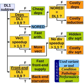
4.7 DL1 Subtree: CPU Performance Evaluation . . . 52
4.8 LS Subtree: Memory Performance Evaluation . . . 53
4.9 OpenMP Performance Subtree . . . 54
4.10 Streams Analysis on PNBench . . . 55
4.11 Group cost analysis on PNBench . . . 56
4.12 Evaluation of the Cost of Cache Coherence Protocol . . . 57
5.1 Exposing the Front-End Ceiling Effect . . . 68
5.2 Modeling the FP Add Functional Unit . . . 70
5.3 Modeling the Store Functional Unit . . . 71
5.4 Impact of TLB Misses . . . 73
5.5 DECAN-level System Saturation . . . 76
6.1 Operating Space of a Performance Prediction Tool . . . 81
6.2 YALES2 loop example . . . 83
6.3 VP3 Projection Results for YALES2: Low Prospects for Vectorization 84 6.5 VP3 Projection Results for POLARIS: VP3 vs. Measurements . . . . 86
6.6 Operating Space of VP3 on POLARIS (θ = 1.2) . . . 86
6.7 VP3 Vec. Projection Steps . . . 87
6.8 Error Cases/16 Validation Codelets vs. θ Tolerance . . . 91
7.1 Realft2_4_de Codelet . . . 98
7.3 Inter-Iteration Dependency Cases . . . 105
7.4 UFS Uop Flow Chart . . . 109
7.5 In Vitro Validation for FP [SNB] . . . 120
7.6 In Vitro Validation for LS [SNB] . . . 121
7.7 In Vitro Validation for REF [SNB] . . . 122
7.8 In Vivo Validation for DL1: Y2 / 3D Cylinder [SNB] . . . 123
7.9 In Vivo Validation for DL1: AVBP [SNB] . . . 124
7.10 UFS Speed Validation for NRs and Maleki Codelets (REF Variant) . 125 7.11 UFS Speed Validation for YALES2: 3D Cylinder . . . 126
7.12 UFS Speed Validation for AVBP . . . 127
A.1 Quantifying Branch Buffer Entries . . . 135
A.2 Quantifying Load Buffer Entries . . . 137
A.3 Quantifying FP PRF Entries . . . 138
A.4 Quantifying Integer PRF Entries . . . 140
A.5 Quantifying Overall PRF Entries . . . 141
A.6 Quantifying ROB Entries . . . 142
A.7 Quantifying RS Entries . . . 144
A.8 Quantifying SB Entries . . . 146
A.9 ROB Microfusion Evaluation . . . 147
A.10 RS Microfusion Evaluation . . . 149
List of Tables
3.1 NR Codelet Suite . . . 28
3.2 Machine List . . . 33
4.1 A few typical performance pathologies . . . 45
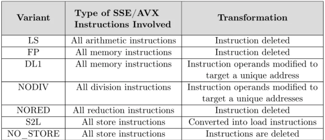
4.2 DECAN variants and transformations . . . 50
4.3 Bytes per Cycle for Each Memory Level (Sandy Bridge E5-2680) . . 53
4.4 PNBench MTL Results . . . 55
5.1 Finding Unlamination Rules . . . 66
5.2 Front-End Stress Experiment Example . . . 67
5.3 Traffic Count Formulas for HSW, SLM and SNB / IVB . . . 72
6.1 BW Scaling Factors (BW Vector / BW Scalar) . . . 89
7.1 Realft2_4_de: Measurements and CQA Error . . . 98
7.2 Realft2_4_de Assembly Instructions . . . 99
7.3 Realft_4_de: Measurements and CQA Error . . . 101
7.4 Exposing Pseudo FIFO limitations: Assembly Code for “rs_pb” . . . 104
7.5 Exposing Pseudo FIFO limitations: Experimental Results . . . 104
7.6 Experimental Resource Quantifying Summary . . . 106
7.7 Partial UFS Loop Input Example (Realft2_4_de) . . . 107
7.8 Needed Resources for Queue Uop Types and Outputs (SNB) . . . 111
7.9 Realft2_4_de: UFS Validation (SNB) . . . 117
7.10 Realft2_4_de UFS Trace . . . 119
7.11 Realft_4_de: UFS Validation (SNB) . . . 120
A.1 Resource Quantifying Experiment Example . . . 134
A.2 Resource Quantifying Experiment Example for the BB (P = 2) . . . 135
A.3 BB Size: Measured vs. Official . . . 135
A.4 Resource Quantifying Experiment Example for the LB (P = 2) . . . 136
A.5 LB Size: Measured vs. Official . . . 136
A.6 Resource Quantifying Experiment Example for the FP PRF (P = 4) 137 A.7 FP PRF Size: Measured vs. Official . . . 139
A.8 Resource Quantifying Experiment Example for the Integer PRF (P = 4) . . . 139
A.9 Integer PRF Size: Measured vs. Official . . . 140
A.10 RQ Experiment Example for the Overall PRF (P = 4) . . . 141
A.11 Overall PRF Size: Measured vs. Official . . . 141
A.12 RQ Experiment Example for the ROB (P = 4) . . . 142
A.13 ROB Size: Measured vs. Official . . . 143
A.14 RQ Experiment Example for the RS (P = 4) . . . 143
A.15 RS Size: Measured vs. Official . . . 144
A.16 RQ Experiment Example for the SB (P = 4) . . . 145
A.17 SB Size: Measured vs. Official . . . 145
A.18 Microfusion Evaluation Experiment for the ROB (P = 4) . . . 147
B.1 Resource Quantifying Experiment Example for the LM (P = 2) . . . 151
B.2 LM Size: Measured vs. Official . . . 152
List of Algorithms
1 Simplified Front-End Algorithm . . . 1102 Issue Algorithm . . . 112
3 Port Binding Algorithm . . . 112
Chapter 1
Introduction
The growing complexity behind modern CPU microarchitectures [1, 2] makes per-formance evaluation and modeling a very complex task. Indeed, modern CPUs will typically implement features such as pipelining, register renaming, speculative and out-of-order execution, data prefetchers, vectorization, virtual memory, caches and multiple execution cores. While each of them can be beneficial to performance, they also make performance analysis more difficult.
On the consumer side of the CPU design process, users want to know which product fits their needs best in terms of performance, energy consumption and/or price. Software developers will be more concerned with adjusting their applications to make the best use of existing features, especially when performance represents a direct competitive advantage.
On the designer side, CPU manufacturers need to build microarchitectures of-fering the characteristics wanted by users while keeping costs low. Furthermore, as product improvements may have to rely on complex mechanisms, they have to guide software developers on how to use them while also having the contrary objec-tive of preventing competitor plagia by controlling the exposure of their performance recipes.
In this context, performance modeling can be used to cost-effectively:
1. Help users find out which hardware would best fit their applications (without actually buying all the considered hardware first).
2. Expose optimization opportunities to software developers (without first testing them).
3. Offer CPU architects insights on which hardware improvements would speed user applications the most (without first implementing them).
This chapter will describe why performance modeling is important in the field of High Performance Computing (HPC) and proceed to present the objectives and contributions of this thesis. It will also provide a quick overview of the document.
1.1
High Performance Computing (HPC)
HPC represents the use of large-scale machines called supercomputers to process compute workloads extremely quickly. It is used (and needed) in areas as diverse as aerodynamic simulations, cryptanalysis, engine design, oil and gas exploration, molecular dynamics or weather forecasting.
It is an environment with very interesting characteristics:
1. Performance is a primary objective and can result in hefty monetary gains. For instance, a faster numerical simulator will be able to provide more results, or/and results of a better quality, in domains as various as the design of cars, plane wings, nuclear plants or the development of new drugs.
2. The used supercomputers can have millions of execution cores [3], offering potentially tremendous calculation speeds and making energy consumption an unavoidable (and expensive) concern: a poorly used machine is a costly machine.
3. Users and software developers can be strongly tied, or even be the same enti-ties. It creates an interesting dynamic where developers are strongly motivated to optimize their code to make the best use of existing resources, and may also have a say in which machines to buy next.
As HPC applications typically spend very large amounts of time in compu-tational loops due to processing large data sets, loop analysis is a primary go-to approach for HPC performance analysis, optimization and modeling.
1.2
Objectives and Contributions
This thesis focuses on increasing the cost-effective observability of potential bottle-necks in HPC computational loops and how they relate to each other. It aims to do so by combining static and dynamic approaches to identify, quantify, and model both the bottlenecks and their interactions.
Its main contributions are:
1. PAMDA, a performance evaluation methodology using a blend of static and dynamic analyses to find bottlenecks and quantify their impact. Its main purpose is to expose optimization opportunities.
2. An adaptation of the Cape linear model to the Sandy Bridge microarchitecture as well as a direct application thereof with VP3, a vectorization gain predictor. 3. Uop Flow Simulation (UFS), a loop performance modeling technique com-bining static analysis and cycle-level simulation to account for out-of-order limitations at a very low execution cost.
Other less significant contributions include:
1. A loop performance measurement framework combining static and dynamic analysis tools to evaluate loop performance from different angles.
2. An empirical approach to quantify out-of-order resources.
1.3
Overview
Chapter 2 will present some background information to familiarize readers with CPU microarchitectural details and nomenclature, performance analysis approaches and tools, as well as with the use of small benchmarks called codelets.
We will introduce a framework combining CQA and DECAN (respectively static and dynamic analysis tools) in Chapter 3. Its objective is to get detailed performance metrics on small codelets given various execution scenarios.
We will then present PAMDA, a performance analysis methodology, in Chap-ter 4. It leverages elements obtained from codelet analysis to detect potential per-formance problems in HPC applications and help resolve them.
1.3. Overview 3
Chapter 5 will describe a work extending the Cape linear model to better cover Sandy Bridge and give it more flexibility for HW/SW codesign purposes. It will be directly used in Chapter 6 with VP3, a tool evaluating the performance gains vectorizing loops could provide.
Chapter 7 will introduce UFS, an approach combining static analysis and cycle-accurate simulation to very quickly estimate a loop’s execution time while accounting for out-of-order limitations in modern CPUs, and better identifying out-of-order related issues than PAMDA or Cape modeling.
We will finally conclude in Chapter 8, summarizing our contributions and pre-senting future work.
Chapter 2
Background
This chapter will focus on presenting the technical context for this thesis and intro-duce some of the nomenclature used throughout this manuscript.
It will first describe modern Intel microarchitectures detailedly, before presenting different performance analysis approaches and tools. It will also explain some of the advantages and limitations of codelets, small benchmarks which we will use for modeling purposes in later chapters.
2.1
Recent Microarchitectures
Microarchitectures are the result of different design choices and incremental im-provements carried over CPU generations. They are typically pipelined and feature the following components:
1. Front-End (FE): component of reading and decoding instructions, making them available to the rest of the execution pipeline.
2. Back-End (BE): executes the instructions provided by the Front-End.
3. Memory Hierarchy: caches can be used to improve the effective speed of mem-ory accesses for both data and instructions.
We will present some of the microarchitectures particularly relevant to HPC here, using information from official sources [4, 5, 6, 7, 8], technical news articles [9, 10, 11, 12, 13, 14, 15], test-based reports [16] and our own observations.
2.1.1 Sandy Bridge
Sandy Bridge (SNB) is a microarchitecture used in the performance-oriented Big Core family of Intel CPUs. It is a tock in the manufacturer’s tick-tock development cycle [17], meaning it keeps the same 32 nm lithography as its Westmere predecessor, but brings important microarchitectural changes.
It will be the microarchitecture this thesis most focuses on. We will present it in details and later use it as a base point to describe the incremental improvements brought by its Ivy Bridge and Haswell successors.
SNB Stock Keeping Units (SKUs) can have from 1 to 6 cores. 2.1.1.1 Front-End
Sandy Bridge’s decode pipeline (also called legacy decode pipeline) is in charge of fetching instructions from the memory hierarchy and decoding them, producing uops more easily interpretable by the Back-End. It is the component the most directly affected by the complexity of the x86 instruction sets, and can produce up to 16 bytes of uop or 4 uops per cycle, whichever is the most restrictive. Furthermore, it has branch prediction abilities, and can decode and provide uops speculatively.
While it can typically only decode up to 4 instructions per cycle, it implements extra features to increase its effective bandwidth:
1. Macrofusion: allows a simple integer instruction and a following branch in-struction to be decoded as a single uop in certain circumstances. This actually brings the maximum theoretical number of decoded instructions to 5 per cycle in favorable corner cases.
2. Microfusion: complex instructions may need to get divided in smaller log-ical operations (or components) when decoded to simplify the Back-End’s work. Microfusion allows instructions having both an arithmetic and a mem-ory components to be fit in a single uop for part of the pipeline despite this constraint, potentially doubling the effective FE bandwidth. For instance, MULPD (%rax), %xmm0 will occupy a single uop slot until each component needs to be executed separately.
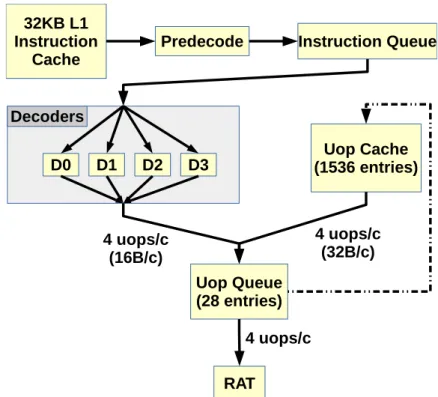
Figure 2.1: Simplified Sandy Bridge Front-End
Sandy Bridge’s Front-End can produce up to 4 uops using any of three different generation mechanisms: the decoders (legacy pipeline), the Uop Cache and the Uop Queue (when iterating over small loops). Only one uop source may be active at a time.
Furthermore, as decoding is a slow and expensive process, Intel CPU architects designed extra mechanisms to prevent instructions from having to be constantly re-decoded, reducing the pressure on the legacy pipeline and increasing the FE’s bandwidth (see Figure 2.1):
1. The uop queue: queues uops right before the RAT, allowing some FE or Back-End stalls to be absorbed. A loop detection mechanism called Loop Stream Detector detects when uops currently in the queue are part of a loop, and can decide to a) stop taking uops from the legacy pipeline, b) not destroy the uops
2.1. Recent Microarchitectures 7
it sends to the Back-End and c) replay them as many times as necessary. While its peak bandwidth is still 4 uops per cycle, there is no limit on the number of transferred bytes anymore, increasing the effective FE bandwidth when lengthy uops are present.
It has a maximum capacity of 28 uops on SNB.
2. The uop cache (or Decoded ICache): it saves uops decoded by the legacy pipeline, and can serve as an alternative uop provider for the uop queue. As with the legacy pipeline and the uop queue, its peak bandwidth is 4 uops per cycle, though with a maximum of 32 bytes of uop being generated per cycle.
It is extremely large compared to the uop queue’s capacity and can contain up to 1536 uops in ideal conditions.
2.1.1.2 Execution Engine
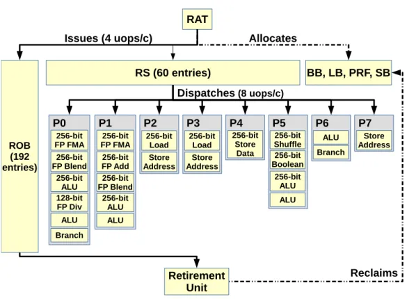
Figure 2.2: Simplified Sandy Bridge Execution Engine
The RAT issues uops from the Front-End to the Back-End after having allocated the necessary out-of-order resources and renamed their operands.
The ROB keeps track of all in-flight uops (both those pending execution and the ones waiting for retirement), while other resources are more specific (e.g. the LB keeps track of load entries). All resources are allocated at issue time and only reclaimed at retirement, with the notable exception of RS entries (which are released once uops are dispatched to compatible execution ports).
The RS can dispatch up to 6 uops per cycle (one to each port) out-of-order. The Resource Allocation Table (RAT) is the gateway component between the
Front-End the FE to the Back-End. It issues uops in-order, performs register re-naming and allocates the resources necessary to their out-of-order execution. While all uops need an entry in the ReOrder Buffer (ROB) to be issued, other out-of-order buffers are allocated on a per-case basis.
Interestingly, not all uops need to be sent to the Reservation Station to wait for execution: Sandy Bridge processes nop uops (which have no input nor output) and zero-idioms (whose output is always zero, and hence have no relevant input) directly in the RAT.
Other resources such as the Branch Buffer, Load Buffer, Physical Registers and Store buffer are intuitively only allocated for respectively branches, loads and soft-ware prefetches, uops with a register output and stores.
Furthermore, with the exception of Reservation Station entries, resources are only released at the retirement step.
The Reservation Station holds uops until their input operands are ready, and then dispatches them to adequate execution ports. The latter will forward them to the proper Functional Units where they will begin their execution.
Most Functional Units are fully pipelined, often giving them a throughput of 1 uop per cycle.
Fully executed uops are retired in-order, at which point their output is committed to the architectural state and their resources freed.
Figure 2.2 summarizes our description of Sandy Bridge’s execution engine.
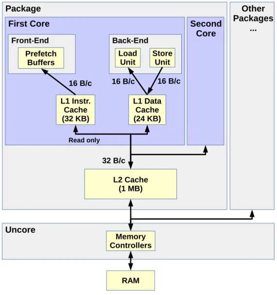
2.1.1.3 Memory Hierarchy
The role of the memory hierarchy is to dampen the impact of RAM’s limited band-width and latency by acting as intermediaries to the main (RAM) memory. Indeed, caches can be much faster than RAM in both regards due to their being much smaller: as a general rule, the smaller the memory unit is, the faster it can perform. CPUs may consequently have several levels of cache, each offering different levels of capacity and performance.
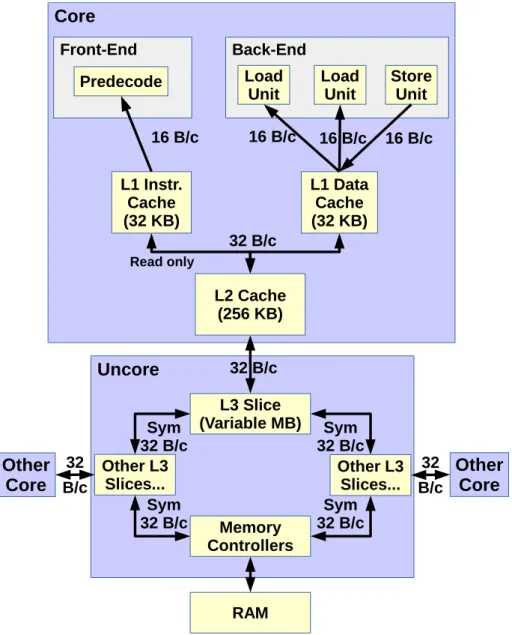
Sandy Bridge’s memory hierarchy is summarized in Figure 2.3.
Load and Store Units can each transfer up to 16 bytes from/to the L1 data cache per cycle, though there are 2 of the former and only 1 of the latter. While they can work concurrently (for an aggregated bandwidth of 24 bytes per cycle), this can only be achieved when using AVX 32-byte vector transfers due to port restrictions (32-byte transfers keep memory units busy for 2 cycles, allowing store address uops to use ports 2 and 3 without penalizing loads).
All of Sandy Bridge’s data caches are write-back: upper cache levels are only made aware of memory writes (or stores) when cache lines from lower levels are evicted. Sandy Bridge’s 32-KB L1 data cache is 8-way associative and virtually indexed. Its 256-KB L2 cache also has an associativity of 8, but is physically indexed and interestingly neither inclusive nor exclusive in regards to L1. The L3’s size is SKU-dependent and can range from 1 to 20 MB. Its associativity is also variable, and is between 12 and 16 depending on the model.
All three cache levels use an NRU (Not Recently Used, a variant of Least Recently Used ) replacement policy.
Four data prefetchers are also present, whose role is to predict which cache lines are going to be needed in the future and request them ahead of time:
2.1. Recent Microarchitectures 9
Figure 2.3: Simplified Sandy Bridge Memory Hierarchy
The data L1 has a combined bandwidth of 48 bytes per cycle, as load and store accesses can be performed in parallel. The L2’s 32 bytes per cycle bandwidth is shared for all fetch and store accesses from the L1s. However, only the data L1 can write data back to the L2. Each L3 slice also has a dedicated bandwidth of 32 bytes per cycle which is shared for read and write accesses from the L2.
The L3 is distributed over all the cores, allowing each core to have their own dedicated access to L3. The bi-directional data ring connecting the slices allows each core to access the entirety of L3, though latency may vary a bit depending on far the relevant slice is.
L3 slices share the same memory controllers for RAM accesses.
1. The DCU Prefetcher (operates in L1): detects ascending-address loads within the same cache line and fetches the following cache line.
2. The Instruction-Pointer-based Prefetcher (operates in L1): detects access stride patterns for individual load instructions and fetches cache lines accord-ingly.
3. The Spatial Prefetcher (or Adjacent Cache Line Prefetcher ; operates in L2): pairs contiguous cache lines in 128-byte blocks. Accesses to the first cache line trigger the fetching of the whole block.
4. The Stream Prefetcher (operates in L2): tries to predict and fetch futurely-used cache lines based on previous accessed addresses. It can keep track of up to 32 different access patterns.
Sandy Bridge has a 2-level Translation Lookaside Buffer system:
1. The L1-TLB is 4-way associative, and can contain up to 64 4KB page entries, 32 2MB entries and 4 1GB entries.
2. The L2-TLB is also 4-way associative, and can contain up to 512 4KB page entries. It cannot hold larger page entries.
2.1.2 Ivy Bridge
Ivy Bridge is the tick improvement of Sandy Bridge, carrying the microarchitecture to a 22 nm lithography but only bringing moderate microarchitectural changes.
IVB CPUs feature from 1 to 15 cores. 2.1.2.1 Front-End
Sandy Bridge’s uses two physical 28-entry uop queues to support hyper-threading. Ivy Bridge improves over it by fusing the queues into a single physical one with 56 entries, and virtually splitting it only when hyper-threading is actually used. It improves its ability to absorb pipeline stalls and increases the maximum size of loops replayable with the Loop Stream Detector, helping improve performance and lower power consumption.
2.1.2.2 Execution Engine
Ivy Bridge introduces 0-latency register moves: in some cases, register moves can be achieved by merely making the named register point to the source physical register, which can be done by the RAT.
The architects also improved the divider / square root unit, likely taking advan-tage of the finer lithography to widen it and improve its bandwidth significantly (as well as its latency to a lesser extent).
2.1.2.3 Memory Hierarchy
While the sizes of L1 and L2 are the same for IVB as for SNB, the maximum L3 size was increased from 20 MB to 37.5.
Furthermore, L3 seems to use an adaptive replacement policy [18].
Ivy Bridge also introduces the Next-Page Prefetcher (NPP), which detects mem-ory accesses nearing the beginning or the end of a page to fetch the matching page translation entry. It is not clear whether the NPP fetches entries to the L2 data cache or directly to the TLBs, though Intel patent [19] suggests the latter.
2.1.3 Haswell
Haswell is the tock after Ivy Bridge, focusing once again on microarchitectural changes and still using the same 22 nm lithography.
2.1. Recent Microarchitectures 11
2.1.3.1 Front-End
Haswell’s Front-End is largely the same as Ivy Bridge’s. 2.1.3.2 Execution Engine
Figure 2.4: Simplified Haswell Execution Engine
The Haswell execution engine brings various improvements over Sandy Bridge, such as more execution ports, new Fused Multiply-Add functional units, larger out-of-order buffers and memory units able to process 32-byte transfers in a single cycle.
The execution engine has some important changes, which are summarized in Figure 2.4. Some of the most important ones include:
1. There now being 8 dispatch ports (against 6 previously), one of which is ded-icated to handle store address uops.
2. Pipelined Fused Multiply-Add units being placed behind ports 0 and 1, dou-bling the potential number of FP operations per cycle. Indeed, they can each execute vector operations such as result = vector1 ∗ vector2 + vector3 with a throughput of 1 per cycle (note: in Haswell’s implementation, the result register must be one of the inputs).
3. The sizes of most out-of-order resources are increased. 2.1.3.3 Memory Hierarchy
The L1 bandwidth is doubled, allowing the two load units and the store unit to each transfer up to 32 bytes per cycle (for a combined bandwidth of 96 bytes per cycle). The L2 bandwidth was also doubled, allowing a full cache line (64 bytes) to be transferred between L1 and L2 every cycle.
The minimum and maximum L3 sizes were increased to reach respectively 2 MB and 45 MB.
Furthermore, some SKUs are equipped with Crystalwell embedded DRAM act-ing as a 128MB L4 victim cache, providact-ing important bandwidth and latency bonuses.
2.1.4 Silvermont
Unlike SNB, IVB and HSW, Silvermont (SLM) is a microarchitecture used for Atom processors, for which emphasis is on low power consumption. Its Bay Trail variant targets the mobile sector, while Avoton micro-server versions were also designed.
Silvermont uses a 22 nm lithography, just like main line processor, and comprises between 1 (in Bay Trail) and 8 cores (in Avoton).
It is a particularly interesting x86 microarchitecture due to how energy con-sumption considerations impacted its design. Furthermore, future high-performance Knights Landing chips will feature around 70 Silvermont-inspired cores, making it very relevant in the HPC sphere.
2.1.4.1 Front-End
Figure 2.5: Simplified Silvermont Front-End
Silvermont’s Front-End can provide the RAT with up to 2 uops per cycle. How-ever, its decoders are limited, and D1 can only decode simple instructions.
A feature called Loop Stream Detector can help compensate for the decoders’ weaknesses when executing loops with small loop bodies, pinning down uops in the Uop Queue and replaying them for as long as possible. The Front-End can then consistently reach its peak bandwidth.
Silvermont’s Front-End supports speculative execution and branch prediction. It is 2-wide (see Figure 2.5), meaning it can decode and provide up to 2 uops to the Back-End per cycle. This is twice less than what Big Core microarchitectures can
2.1. Recent Microarchitectures 13
do, and is further aggravated by SLM’s individual instruction decoders being less potent than those in the main line products. They are however more power-efficient. There is also a Loop Stream Detector in the uop queue, which takes a very high importance due to the decoders’ weaknesses. While for SNB/IVB/HSW using the LSD is done rather opportunistically, it is an important factor for SLM performance. 2.1.4.2 Execution Engine
The RAT / Allocation / Rename cluster bridges the FE with the BE, inserting uops in-order after a) allocating some of the necessary resources for their execution and b) renaming their input and output registers.
All uops need an entry in the ROB. It is also not clear when other resources (e.g. Load Buffer) are allocated, as Intel claims Silvermont uses a late allocation / early resource reclamation scheme [20].
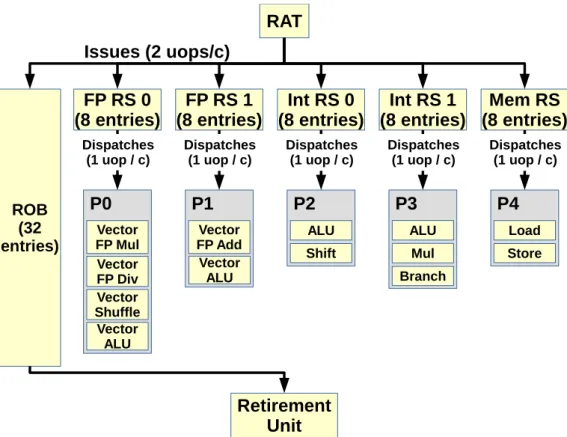
The scheduler system is distributed over different Reservation Stations, each handling a specific execution port (see Figure 2.6), and their own in-order or out-of-order dispatch policy:
1. FP RS 0: handles FP and vector additions, as well as some other arithmetic and logic operations. Dispatches uops in-order (only in regards to uops in FP-RS-1).
2. FP RS 1: handles FP and vector multiplications, divisions, shuffles and other operations. Dispatches uops in-order (only in regards to uops in FP-RS-2). 3. Int RS 0: handles integer arithmetic, logic and shift operations. Dispatches
uops out-of-order.
4. Int RS 1: handles integer arithmetic and logic as well as branches. Dispatches uops out-of-order.
5. Mem RS: handles address generations, loads and stores. Dispatches uops in-order, but allows accesses to complete out-of-order to absorb latency.
Fully executed uops are retired and committed in-order. 2.1.4.3 Memory Hierarchy
Silvermont has a 24KB L1 with an associativity of 6. The load and store units can transfer up to 16 bytes per cycle from/to it, though they likely cannot do so simultaneously (as only one address per cycle can be generated for loads and stores). It adopts a random cache line replacement policy.
Single-core Silvermont SKUs have a 512KB L2.
SKUs with more than 1 core are organized in pairs of cores called modules, with each module having 1 MB of dedicated 16-way associative L2. The overall cache size for 8-core Silvermont CPUs hence reaches 4 MB, though each core is constrained to only use the L2 slice from its own package.
The L1 and the L2 can exchange up to 32 bytes per cycle, though this link is shared with all the cores in the package. It uses an NRU cache line replacement policy.
The L1 and L2 caches are both write-back.
There are two data prefetchers, the L1 Spatial Prefetcher and an L2 “advanced” prefetcher. They are likely respectively inspired by the L1 DCU and the L2 Streamer prefetchers from the Big Core CPUs, but not many details are given.
Figure 2.6: Simplified Silvermont Execution Engine
Unlike Big Core microarchitecture, there is no unified reservation station. Fur-thermore, each small RS acts with its own rules:
1. The FP Reservation Stations have to dispatch their uops in-order.
2. The Mem RS also has to dispatch uops in-order (to help memory scheduling be as simple as possible), but they are non-blocking and can be be completed out-of-order.
3. Integer Reservation Stations can dispatch uops out-of-order.
The ports presented here might not actually have a discrete existence, (as absent from any official documentation we could find), but we decided to put them here anyway to simplify the figure. We labelled them in a manner consistent with Big Core CPUs.
Silvermont also has a 2-level TLB cache:
1. The L1 TLB has 48 4KB entries and is fully associative.
2. The L2 TLB has 128 4KB entries and 16 2MB entries, and is 4-way associative. It is not inclusive (nor exclusive) in regards to the L1.
Figure 2.7 summarizes this memory hierarchy.
2.2
Performance Analysis
Different approaches can be adopted to analyze performance, each working with their own tradeoffs. This section will present some of them.
2.2. Performance Analysis 15
Figure 2.7: Simplified Silvermont Memory Hierarchy
The Load and the Store units cannot access L1 in parallel, so the data L1’s bandwidth is of 16 bytes per cycle.
The L2 cache space and bandwidth are shared between cores from a same pack-age.
Finally, the memory controllers are shared by all cores on the CPU.
2.2.1 Static Analysis
Static analysis consists in evaluating software without executing it. This offers the advantage of being particularly fast, at the cost of working with a limited amount of information.
We will present tools using this approach in this section.
2.2.1.1 Code Quality Analyzer (CQA)
CQA [21] evaluates the quality of assembly loops and projects their potential peak performance. It is developed inside the MAQAO [22] framework, which handles both the disassembling of target compiled binaries and the detection of the loops within.
1. The evaluated code is the code executed by the machine. This is not (neces-sarily) when working at the source level due to the optimizations the compiler can apply.
2. Loop instructions can be tightly coupled to known microarchitecture features and functional units, making performance estimates solidly grounded in reality. However, assembly-level static analysis does not (consistently) allow to detect and account for issues such as poor memory strides, which could have been observed in the source code.
CQA’s metrics include:
1. Peak performance in L1 (assuming no memory-related issues, infinite-size buffers and an infinite number of iterations).
2. Front-End performance.
3. Distribution of the workload across the different ports and functional units. 4. Vectorization-efficiency metrics.
5. Impact of inter-iteration dependencies.
CQA can also provide suggestions on how to fix detected performance problems.
2.2.1.2 Intel Architecture Code Analyzer (IACA)
IACA is also a static analysis tool working at the assembly level. Unlike CQA, it uses markers inserted at the source level to locate the code to analyze. It allows users to easily target the parts they want analyzed, but forces them to place these markers and recompile their application.
Two types of analyses are possible:
1. Throughput analysis: the target block of code is treated as if it were a loop for the purpose of detecting inter- iteration dependencies, and evaluates per-formance in terms of instruction throughput. (This analysis is very close to CQA’s, though with the extra assumption that the Front-End can always deliver 4 uops per cycle.)
2. Latency analysis: IACA evaluates the number of cycles needed go executed the target block once.
In both cases, IACA can highlight the assembly instructions that are are part of the performance bottleneck.
2.2.2 Dynamic Analysis
Dynamic analysis uses runtime information to evaluate performance. It can pro-vide large amounts of information not obtainable through purely static means, but typically requires the target program to be executed at least once.
Furthermore, it introduces problems of its own, such as measurement stability and precision.
2.2. Performance Analysis 17
2.2.2.1 Hardware Support
Hardware can implement features specifically intended for performance evaluation. They can allow dynamic analysis to be faster, easier, more precise and/or collect more relevant information.
The Time Stamp Counter [23] (TSC) provides a very precise way of measuring time at a very low cost. Indeed, it counts the number of spent cycles, and is readable in only around 30 cycles using the RDTSC instruction on Sandy Bridge, making it very cost-effective.
Performance Monitoring Counters [24] can also count events other than just cycles, such as the number of retired instructions, the number of cache lines read from RAM, the number of stalls at different stages of the execution pipeline or even power consumption. All this information can be obtained through other means (value tracing, simulation, hardware probes), but at a much higher complexity and cost.
Furthermore, different methods can be used to access these counters:
1. Sampling: counters are parameterized to keep track of certain events and raise an interrupt when a certain threshold is reached. Sampling software can then identify the last retired instruction and credit it for the overflown counter’s events, reset said counter to 0 and resume the program’s execution. It is a very cheap and non-intrusive way to collect performance counter data. 2. Tracing: sampling’s precision is not perfect as it essentially works by “blaming”
the instruction that caused the overflow for the entirety of the event sample without any guarantee that it is indeed responsible for a majority of them. Furthermore, it cannot dissociate events associated to the same code but in different execution contexts (e.g. different function parameters). Tracing ad-dresses these concerns by inserting start and stop probes in strategic parts of the code (e.g. right before and after a loop), allowing to a) precisely count events caused by the loop, and only by the loop and b) separate events caused by the same code area but at different times. It however comes at a higher cost because probes need to be inserted in the first place, and is not a working solution for tiny pieces of code.
3. Multiplexing: multiplexing consists in using the same hardware counter to monitor more than one event. It is done by making the counter alternate between the watched events during the measurement phases. It allows to collect more counters simultaneously (as the number of monitoring units is limited), but can degrade the precision of results.
However, the overhead for accessing PMCs can be important and should be considered when using them [25].
2.2.2.2 Finding Hotspots
Finding an application’s hotspots (i.e. parts of the program needing the most time to execute) is important for performance analysis and optimization as it allows tools and developers to focus on parts of the code that have an important impact on the overall execution time. Different techniques can be used to find them.
For instance, Intel compilers have an option to insert RDTSC probes in the assembly code, tracing the time spent in different loops and functions [26]. The
main drawback of this method is that it requires having access to the source code (and recompiling it for performance monitoring purposes).
Tools such as VTune [27] and Perf [28] can detect hotspots using sampling. The Perf module of MAQAO [29] can also do so in applications using OpenMP or OpenMPI frameworks. Though this technique is not perfect [30], it is very efficient and does not require any changes to be made to the target application.
2.2.2.3 Counter-based Analysis
Programs or frameworks such as Oprofile [31], PAPI [32] and Likwid [33] only per-form PMC measurements, leaving the analysis to other tools.
VTune [27] is a special case and combines both measurement and analysis abil-ities. Among them, the Top-Down approach [34] evaluates the performance contri-butions of the Front-End, Back-End, retirement and memory accesses.
Levinthal [35] offers counter-based performance metrics to evaluate performance bottlenecks.
HPC oriented frameworks [36] can also detect and categorize performance issues in parallel applications, as well as suggest potential fixes such as in-lining functions or changing data structures.
2.2.2.4 Differential Analysis
Differential Analysis [37] consists in a) transforming a given target code to isolate some of its characteristics and b) comparing the execution times of the original and the modified codes to evaluate the impact of the targeted characteristics.
DECAN is a tool implementing this approach at the assembly loop level. It was developed within MAQAO [22], using the framework’s binary patching features [38] to generate new binaries with modified loops.
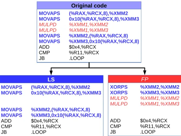
Figure 2.8 show-cases its main transformations:
1. LS (Loads/Stores): only keep memory instructions, address calculations and control flow instructions (which are necessary for the loop to iterate normally). Running this variant allows to see the contribution of memory accesses to the original loop’s execution time.
2. FP (Floating Point): only keep floating point instructions and the control flow. It isolates the impact of FP operations in the original loop.
DECAN can be used on sequential, OpenMP and MPI programs alike.
One of the drawbacks of this approach is overhead, as each of the the target loop’s variants need to be executed.
2.2.3 Simulation
Simulation can bring information that is difficult or impossible to otherwise get, and is often used as a means of validating performance models when the modeled hardware does not exist, or is hard to access.
However, it is a complex process for which one of the trade-offs is nearly always execution time, though other factors (e.g. memory consumption) may also get in the picture.
2.2. Performance Analysis 19
Figure 2.8: Example of DECAN Loop Transformations
This example assembly code multiplies all elements from an array by a constant. DECAN can be used to patch loops to isolate some of their performance char-acteristics.
In the LS version, the MULPD floating point instructions were removed. In the FP version, loads were transformed into zero-idiom XORPS instruc-tions to avoid creating new dependencies on the XMM registers. Stores were simply removed.
2.2.3.1 Simulation Techniques
Different techniques can be used depending on the objectives of the simulation, or the targeted performance trade-off.
Execution-driven simulators [39, 40] simulate both the semantic of a program and its behavior on the modeled system. It allows them to tackle problems from scratch, but at high cost.
Trace-driven simulation offsets part of the problem by first collecting relevant execution details [41] (e.g. the list of all instructions executed for a program, as well as their outputs), and then using these traces to reconstitute the program’s semantics. The simulation then only targets the behavior of the traced instructions, allowing it to be both less complex and faster than an execution-driven equivalent. However, trade-offs for using this technique include a) having to run the target program on a real machine (or an execution-driven simulator...) at least once to collect the traces, b) storing and using
trace files which can be extremely large and c) not being able to see the impact of e.g. randomness or different instruction sets without getting different traces.
Simulators can also have varying scopes. Full-system simulators [42, 43, 44] will simulate not just the CPU, but also other components such as graphical cards or
network cards so as to be able to run entire operating systems. However, their main objective is more likely to enable e.g. driver development for not-yet-existing hardware or system-level performance analysis, taking their focus further away from pure CPU performance analysis. PTLsim [45] adopts an interesting approach com-bining virtualization and simulation for performance analysis, allowing users to use virtualization’s near-native execution speed when speed is important, and switching to simulation mode for performance analysis.
2.2.3.2 Cycle-Accurate Simulation
Detailed cycle-accurate simulation is the only way to get a perfect knowledge of a system’s performance. It offers a full visibility on all relevant mechanisms without any impact on the results (unlike hardware or software measurement probes).
However, it comes with several drawbacks:
1. Execution time: simulators modeling everything perfectly will typically sim-ulate at rates of a few thousand cycles per second [46], which represents a slowdown in the order of millions.
2. Amount of data: it can be hard to know which parts of the modeled system are actually relevant, and tell the cause from the consequence: simulation does not supersede analysis.
3. Purely simulation-based analysis can be very slow, as each tested potential bottleneck has to be tested separately and result in whole new simulation run. Furthermore, cycle-accurate simulators modeling all the details of modern CPUs’ hardware implementations are not publicly available, limiting their applicability for performance analysis for general application developers.
2.2.3.3 Improving Simulation Speeds
Different approaches have been developed to improve the speed of simulation: 1. Sampled simulation [47, 48]: simulating only parts of the execution in details
allows to use faster techniques (e.g. emulation) for most of the time. The quality of the results will then depend on the sampling rate, and the quality (representativeness) of the samples.
2. Using dedicated simulation hardware [49, 50]: using FPGAs can greatly help with achieving better simulation speeds, as the hardware running the simula-tion is specifically fine-tuned for this task.
3. Interval simulation [51]: focuses on modeling the impact of miss events (e.g. cache miss, branch misprediction) and uses a simplified, fast model for the rest of the execution.
2.2.3.4 Functional Simulation
Specialized functional simulators can also provide interesting information. Such tools focus on reproducing realistic behaviors with no particular regards for timing. For instance, tools like Cachegrind [52] track memory accesses and replay them in a realistic cache structure, evaluating how and whether programs use caches. Other tools [53] can also characterize multi-threaded workloads.
2.3. Using Codelets 21
2.3
Using Codelets
Tackling important problems can often be simplified by decomposing them into smaller ones, which are more easily understood and fixed. The codelet approach applies this principle to modeling and optimization problematics, focusing on smaller problems to then approach the bigger ones.
2.3.1 Codelet Presentation
Codelet definitions may vary depending on their granularity and purposes. We will hence clarify our use of the term, as well as some of codelets’ main advantages and drawbacks.
2.3.1.1 Definition
A codelet is a small piece of code that may be evaluated independently. Codelets can be coupled to drivers, intendedly minimal code complements allowing them to be run in a stand-alone manner.
In the context of this thesis, codelets will always be loop nests. However, coarser-grain codelets like functions could also be used.
2.3.1.2 Why use codelets?
Whether or not codelets are interesting depends on their intended uses:
1. For modeling, they are particularly interesting if they display some novel or/and unexpected behavior, as their being small helps pinpoint the issue. 2. For optimization, codelets can isolate significant performance problems,
allow-ing potential solutions to be tested in a vacuum.
3. HPC scheduling: codelets could be used as a finer schedulable workload than threads [54], allowing to make better use of supercomputers’ very high numbers of cores.
Codelets can offer important advantages in both cases:
1. Evaluating the impact of the environment: codelets’ behavior variations de-pending on the execution environment (e.g. different host machines or CPU operating frequencies) can be determined in a cost-effective way due to their stand-alone nature and their normally small execution times.
2. Varying data sets: some codelets may allow for arbitrary input data sets to be used, making it possible to see how their behavior evolves with varying cache localities.
3. Optimization tests: codelets being stand-alone programs allows programmers to test different optimizations (or compiler optimization flags, compiler ver-sions, etc.) and only impact the intended code. It would not be as simple with e.g. real applications, in which potential optimizations may have an impact on the whole program.
2.3.1.3 Drawbacks of Codelets
While codelets may be very convenient, their stand-alone property may raise prob-lems such as:
1. Static interference: the compiler may alter or reorder statements to try to produce more efficient code (e.g. loop interchanging, in-lining...), or certain optimizations may be overly optimistic (e.g. optimizing data structures for individual loops whilst they are used for a whole program). Studying a piece of code out of its original (or a realistic) context may hence create unnatural circumstances.
2. Cold/warm cache [55]: the state of the caches when running a codelet may have a strong impact on its observed behavior. Several possibilities exist (com-pletely cold caches, com(com-pletely warm ones, or various degrees in-between). As there is no universal strategy to create a single most-appropriate execution en-vironment, users have to make this potentially complex decision on a per-case basis.
3. Dynamic influence from and on other loops: in a real application, a loop may have a strong influence on how other loops behave and in turn be influenced by other loops’ execution. For instance, a previous loop could warm up caches or on the contrary trash them, and instructions from different loops can also cohabit in the execution pipeline due to superscalar mechanisms. Combining the codes of two codelets together may hence produce different results than when running them separately.
These issues may ultimately cause modeling or optimization projection errors. They represent a limitation that codelet users should keep in mind.
2.3.2 Artificial Codelets
Developing artificial codelets allows for a fine control of experiments. However, they require codelet creators to already have a clear idea about what they want to test, and how.
2.3.2.1 Hand-Crafted Codelets
Some codelets can be handmade to test something specific. Furthermore, small benchmarks do fit our definition of codelet.
On the hardware side, [56, 57] use simple benchmarks to characterize the effective bandwidth on a machine. [57] also covers other potential bottlenecks such as memory latency or network bandwidth.
On the software side, [58, 59] use handmade (and legally vectorizable) loops to test auto-vectorizing compilers’ abilities.
2.3.2.2 Automated Generation
Codelets can also be generated automatically, following patterns of (potential) in-terest. Microtools [60] facilitate this process to evaluate the impact of e.g. different memory access patterns, unrolling or vectorization. They can also measure the execution times of the resulting codelets.
2.3. Using Codelets 23
Henri Wong [61] generates loops using pointer-chasing to expose the number of out-of-order resources in the ROB and the Physical Register File in Intel microar-chitectures, as well as test the impact of zero-idiom and register move instructions on register consumption.
2.3.3 Extracted Codelets
Codelet extraction is the process of isolating a program’s hotspot as a codelet. Such codelets offer various advantages over synthetic ones:
1. They represent realistic workloads. For instance, on SNB, there is an impor-tant penalty for using both SSE and AVX instructions in the same loop. While a synthetic codelet will be able to exactly address this problem, mixing such instructions is not a mistake compilers would do in realistic circumstances, hence much lowering its relevance. Extracted codelets will expose real day-to-day problems and bottlenecks.
Having realistic workloads allows models to be trained on codes directly rele-vant to their objectives (e.g. using HPC codelets to model HPC applications). 2. They can be used to study each of an application’s hotspots separately, allow-ing said application’s performance to be modeled in small bricks rather than as a whole [62].
2.3.3.1 Manual Extraction
Codelets can be extracted manually, e.g. by copying the source code of a loop. However, it is a slow and error-prone process which can only be reasonably used when the number of interesting codelet candidates is low.
However, it is a fairly simple process, and allows for implementation liberties e.g. to allow arbitrary data sets to be processed by the loop.
2.3.3.2 Automated Extraction
Automating the extraction process greatly reduces the costs of codelet extraction, as well as the hazards inherent to manual processing. It also makes it realistic to cover the majority of the execution time in HPC applications potentially comprising hundreds of hotspots.
Codelet extraction tools can operate at different levels. For instance, [63, 64, 65] extract hotspots at the source level, also saving the runtime state of the memory so that the resulting codelet can be replayed faithfully. A drawback of this method is that there may be discrepancies between the generated compiled codes for original and extracted versions.
On the other end of the spectrum, [66] identifies codelet-like structures called simulation points. They are pieces of code pinpointed at the assembly level for the purpose of speeding up simulation. This technique is extremely faithful in terms of assembly code and memory states, but limits the adaptability and portability of the identified workloads.
An in-between approach is adopted in [67], where hotspots are extracted at a compilation-time Intermediate Representation (IR) level. It offers advantages in terms of extraction complexity as the IR may be language-independent, but creates a dependency on the used compiler instead. Unlike source-level extraction, it does not
allow for codelets to be easily modified, but is more flexible than Simulation Points as it allows for different optimization flags and data sets to be tried. [68] adapts this approach to parallel codes, operating at a coarser granularity to quickly evaluate the scalability of OpenMP parallel regions.
Chapter 3
Codelet Performance
Measurement Framework
The complexity of modern CPUs makes loop performance be the result of many factors simultaneously coming into play. Identifying these factors, their individual impact and how they interact with one another correspondingly becomes increas-ingly difficult.
In this chapter, we approach this issue by producing fine-grained data on vari-ous -but mostly simple- loops in a controlled in vitro environment. The aim is to produce reliable data allowing to single out certain components’ behavior, check implementation hypotheses and validate low-level performance-evaluation tools.
3.1
Introduction
Modern CPUs being developed in a highly competitive and industrial environment, pushing companies into different strategies to protect their competitive advantage:
1. Patenting: while offering legal protection against plagia, patents have the downsides of a) only protecting implementations, b) requiring the publication of the material to protect and c) being temporary. Furthermore, as they can be costly to establish, not all innovative solutions may be deemed worth the matching cost.
2. Secrecy: confidentiality can protect ideas (outside the realm of patentable ma-terials), but very little can be done against plagia if the material gets leaked or stolen. This forces companies to be conservative in terms of releasing technical implementation details.
In this environment, performance researchers have to deal not just with the complexity brought by state-of-the art CPUs comprising billions of transistors, but also with the unknowns induced by hardware characteristics not disclosed by CPU manufacturers.
We specifically target Intel microarchitectures, for which the manuals provided by the manufacturer still provide a sizeable amount of information on microarchitec-tures’ pipeline and hence allow for a reliable overview of the core pipelines. Further to this, information from patents can provide interesting leads on implemented hard-ware mechanisms, though patents can exist without the mechanisms they describe being actually implemented in real-world products.
Empirical data can be used to:
1. Independently validate information from manuals.
2. Test implementation hypotheses (and empirically expose undocumented char-acteristics).