On Microelectromechanical Systems with General Permittivity

(1)

HAL Id: tel-01325059

https://tel.archives-ouvertes.fr/tel-01325059

Submitted on 1 Jun 2016

HAL is a multi-disciplinary open access archive for the deposit and dissemination of sci-entific research documents, whether they are pub-lished or not. The documents may come from teaching and research institutions in France or abroad, or from public or private research centers.

L’archive ouverte pluridisciplinaire HAL, est destinée au dépôt et à la diffusion de documents scientifiques de niveau recherche, publiés ou non, émanant des établissements d’enseignement et de recherche français ou étrangers, des laboratoires publics ou privés.

On Microelectromechanical Systems with General

Permittivity

Christina Lienstromberg

To cite this version:

Christina Lienstromberg. On Microelectromechanical Systems with General Permittivity. Solid me-chanics [physics.class-ph]. Université Paris-Saclay; Universität Hannover, 2016. English. �NNT : 2016SACLN007�. �tel-01325059�

(2)

On Microelectromechanical Systems

with General Permittivity

Christina Lienstromberg

Thèse de Doctorat en Cotutelle

entre l’Université Paris-Saclay et Leibniz Universität Hannover, préparée à l’École Normale Supérieure de Cachan, Laboratoire de Mécanique et Technologie et Fakultät für Mathematik und Physik, Institut für Angewandte Mathematik pour obtenir le grade de Docteur de l’Université Paris-Saclay

École doctorale N◦_{579: Sciences mécaniques et énergétiques, matériaux et géosciences.}

Spécialité: Mécanique des solides.

Numéro national de thèse: 2016SACLN007.

Présentée et soutenue à Hanovre le 22 janvier 2016 devant le jury composé de : Marc Steinbach Professeur, Leibniz Universität Hannover Président

Adrian Constantin Professeur, Universität Wien Rapporteur et examinateur Gerhard Starke Professeur, Universität Duisburg-Essen Rapporteur et examinateur Elmar Schrohe Professeur, Leibniz Universität Hannover Rapporteur et examinateur Pierre Gosselet Chargé de recherche, CNRS/ ENS de Cachan Directeur de thèse

Joachim Escher Professeur, Leibniz Universität Hannover Directeur de thèse

(3)

(4)

iii

Acknowledgements

Above all, I express my sincere gratitude to Joachim Escher for proposing the research topic and for his faithful support and advice.

In addition, I am grateful to Pierre Gosselet for his helpfulness during my stay at the ENS Cachan and to Gerhard Starke for fruitful discussions and for drawing my interest to the field of numerical analysis. Further thanks go to Adrian Constantin and Elmar Schrohe for reviewing this dissertation. The financial support by the DFG IRTG 1627 is also kindly acknowledged.

I am very thankful to the members of the Institute of Applied Mathematics for an inspiring environ-ment and excellent working conditions. Particular thanks go to my colleagues and friends Gabriele Brüll, Davide Veniani, Jan Thiedau and Jacques Jabbour for their cordial friendship.

Moreover, I like to take the opportunity to thank Anni, Isa, Aki and JJ for their friendship and for spending a great time at the 3rd floor.

(5)

(6)

v

Zusammenfassung

Gegenstand der vorliegenden Arbeit ist die mathematische Untersuchung von Systemen gekoppelter partieller Differentialgleichungen, die von der Modellierung elektrostatisch betriebener mikroelek-tromechanischer Systeme mit allgemeiner Permittivität herrühren. Eine Herleitung verschiedener Modelle wird vorgestellt, die es dem Leser ermöglicht, eine Einsicht in die diversen physikalischen As-pekte zu erlangen, die entsprechend der jeweiligen Anwendung in Betracht gezogen werden können. In jedem Fall koppeln alle adäquaten Systeme ein entweder semi- oder quasilineares hyperbolisches oder parabolisches Evolutionsproblem für die Auslenkung einer elastischen Membran mit einem el-liptischen freien Randwertproblem, das das elektrostatische Potential in dem Gebiet zwischen der elastischen Membran und einer starren Bodenplatte determiniert.

In der Folge wird das qualitative Verhalten der Lösungen zweier verschiedener gekoppelter Probleme studiert. Genauer beinhalten beide betrachteten Systeme das elliptische freie Randwertproblem zur Bestimmung des elektrostatischen Potentials, das lediglich entsprechend der Wahl des Permittiv-itätsprofils variiert. Eher kleine oder große Auslenkungen der Membran beschreibend, kommt ein entweder semi- oder quasilineares parabolisches Evolutionsproblem hinzu. Für beide Systeme wird gezeigt, dass sie für alle beliebigen positiven Werte λ der angelegten Spannung lokal bezüglich Zeit wohlgestellt sind. Kleine Werte λ der angelegten Spannung, die einen gewissen kritischen Wert λ⇤ nicht überschreiten, lassen sogar global in der Zeit existierende Lösungen zu. Im semilinearen

Fall wird für ein gegen Null konvergierendes Längenverhältnis des Geräts Konvergenz der Lösungen des vollen gekoppelten Problems gegen diejenigen des entkoppelten sogenannten Small-Aspect Ratio Models nachgewiesen.

Des Weiteren wird ein Thema behandelt, das erst mit der Berücksichtigung nicht-konstanter Permit-tivitätsprofile Bedeutung erlangt – die Richtung der Membranauslenkung oder, in mathematischer Ausdrucksweise, das Vorzeichen der Lösung des Evolutionsproblems. Mit Hilfe des parabolischen Vergleichsprinzips werden strukturelle Bedingungen an das Potential sowie das Permittivitätsprofil spezifiziert, die Nicht-Positivität der Membranauslenkung garantieren. Für gewisse Permittivitäts-profile wird schließlich bewiesen, dass Singularitäten nach endlicher Zeit auftreten können, sobald die angelegte Spannung einen bestimmten kritischen Wert λ⇤_{überschreitet. Die Arbeit schließt mit}

einer numerischen Analyse des semilinearen Problems, die insbesondere die Betrachtung des vollen gekoppelten Problems rechtfertigt, indem sie wesentliche qualitative Unterschiede zwischen den Lö-sungen des weitverbreiteten Small-Aspect Ratio Models und denen des vollen gekoppelten Modells aufzeigt.

Schlüsselwörter: Mikroelektromechanische Systeme (MEMS), Permittivität, partielle Differ-entialgleichungen, freie Randwertprobleme, nichtlineare Evolutionsgleichungen, Singularitäten nach endlicher Zeit

(7)

(8)

vii

Abstract

Of concern is the mathematical investigation of systems of coupled partial differential equations arising from the modelling of electrostatically actuated microelectromechanical systems with gen-eral permittivity profile. A derivation of different models is presented that enables the reader to establish an understanding of the various physical modelling aspects that might be taken into ac-count according to the particular application. Howsoever, all suitable systems couple an either semi-or quasilinear hyperbolic semi-or parabolic evolution problem fsemi-or the displacement of an elastic membrane with an elliptic moving boundary problem that determines the electrostatic potential in the region between the elastic membrane and a rigid ground plate.

Subsequently the qualitative behaviour of the solutions of two different coupled problems is studied. More precisely, both systems under consideration consist of the elliptic free boundary problem for the determination of the electrostatic potential, which varies solely according to the choice of the permittivity profile. Describing rather small or large deflections of the membrane, an either semi- or quasilinear parabolic evolution problem is added. Both systems are shown to be well-posed locally in time for all arbitrary positive values λ of the applied voltage. Small values λ of the applied voltage, that do not exceed a certain critical value λ⇤, do even allow globally in time existing solutions. For

the semilinear case we establish the convergence of solutions to the full coupled problem towards those of the decoupled so-called small-aspect ratio model, as the aspect ratio of the device tends to zero.

Furthermore, a topic is addressed that is of note not till non-constant permittivity profiles are taken into account – the direction of the membrane’s deflection or, in mathematical parlance, the sign of the solution to the evolution problem. By means of the parabolic comparison principle structural conditions on the potential and on the permittivity profile are specified which guarantee non-positivity of the membrane’s displacement. For certain permittivity profiles we finally prove that finite-time singularities may occur as soon as the applied voltage exceeds a certain critical value λ⇤_{. We complete the work by a numerical analysis of the semilinear problem that in particular}

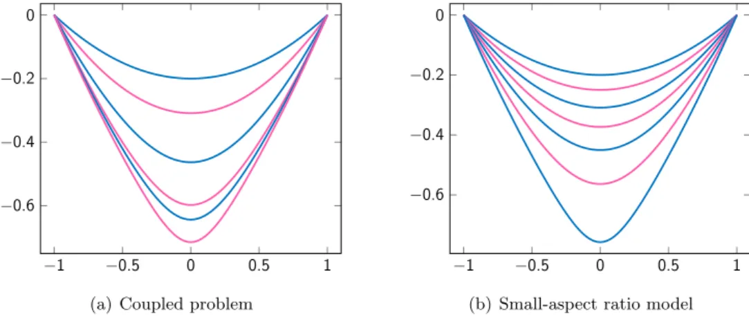
justifies the consideration of the full coupled problem by revealing substantial qualitative differences of the solutions to the widely-used small-aspect ratio model and the full coupled problem.

Keywords: Microelectromechanical systems (MEMS), permittivity, partial differential equations, free boundary value problem, nonlinear evolution equations, finite-time singularities

(9)

(10)

ix

Résumé

La thèse concerne l’investigation mathématique des systèmes d’équations aux dérivées partielles cou-plées, qui découlent de la modélisation des microsystèmes électromécaniques avec une permittivité générale. Une dérivation des différents modèles est présentée, ce qui permet au lecteur d’acquérir une compréhension des nombreux aspects physiques qui peuvent être pris en considération confor-mément à l’application visée. Quoi qu’il en soit, tous les systèmes appropriés couplent une équation d’évolution semi- ou quasilinéaire qui est soit hyperbolique soit parabolique pour modéliser la défor-mation d’une membrane élastique et un problème elliptique à frontière libre. Ce dernier détermine le potentiel électrique dans la région située entre la membrane élastique et une plaque à la masse. Ci-après le comportement qualitatif des solutions de deux différents problèmes couplés est étudié. Plus précisément, les deux systèmes considérés se composent d’un problème elliptique à frontière libre pour la détermination du potentiel électrique, qui varie exclusivement en fonction du choix du profil de permittivité. Un problème d’évolution parabolique semilinéaire ou quasilinéaire est ajouté, décrivant respectivement des petites ou des grandes déformations de la membrane.

Il est montré que les deux systèmes sont localement bien posés dans le temps pour n’importe quelle valeur λ > 0 de la tension électrique appliquée. Pour de petites valeurs λ de la tension électrique appliquée, n’excédant pas une certaine valeur critique λ⇤_{, permettent même une solution unique}

qui existe globalement et pas que localement. Pour le cas semilinéaire la convergence des solutions du problème couplé vers celles du modèle élancé (small-aspect ratio model) est établie, lorsque le rapport hauteur/largeur tend vers zéro.

De plus, l’utilisation de profils de permittivité non-constants rend non-triviale l’étude du signe de la solution du problème d’évolution ou en termes mécaniques l’étude de la direction de la déformation de la membrane. En employant le principe du maximum parabolique des conditions structurelles au potentiel et au profil de permittivité sont spécifiées pour garantir la non-positivité de la déformation de la membrane. Enfin, la formation de singularités en temps fini pour certains profils de permit-tivité du moment que la tension électrique excède une certaine valeur critique λ⇤ _{est prouvée. Le}

travail est terminé par une analyse numérique du problème semilinéaire, qui en particulier justifie la considération du problème entier couplé en démontrant des différences qualitatives entre les solutions du small-aspect ratio model communément utilisé et celles du problème couplé.

Mots clés: Microsystèmes électromécaniques (MEMS), permittivité, équations aux dérivées partielles, problème à frontière libre, équation d’évolution nonlinéaire, singularités en temps fini

(11)

(12)

1 | Introduction

Moving boundary problems or synonymously free boundary value problems frequently arise in a natural way when describing complex physical or chemical phenomena in nature and technique. They denote systems of partial differential equations which are in particular characterised by the fact that they are to be solved for a domain whose boundary is not known a priori and thus itself constitutes a part of the solution. Due to this coupling between the components of the full solution moving boundary problems are inherently nonlinear, making their analytical and numerical investigation evidently rather involved. On the other hand their intricate and nonlinear nature provides a more accurate description of complex processes than linear or nonlinear models on fixed domains. As a consequence in the last decades the investigation of moving boundary problems has received remarkable attention in applied mathematics. In this spirit, the present thesis is devoted to an analysis of free boundary value problems describing the dynamic behaviour of microelectromechanical systems.

Microelectromechanical systems (MEMS) constitute a technology of miniaturised devices whose dimensions range between some micrometres and one millimetre. Being typically made up of a sensor, a transistor as well as a mechanical actuator, MEMS sense the environment and act on it by combining microelectronics with non-electronic activities from micromechanics, fluidics or optics. Whereas the component of microsensors is already well developed, the understanding and construction of microactuators still pose a challenge and thus also deserve study in different fields of science [9]. The underlying technology is based on the approach of generating mechanical motion by for instance electrostatic, thermal, hydraulic, magnetic or other forces which act by reason of a perception of the environment by a sensor.

Due to their low manufacturing costs, their low demand for energy, their high reliability and in particular their tremendous versatility, MEMS have found their way into numerous branches of industry and science. The automotive industry, telecommunications or the biomedical industry shall be instanced here in order to provide an insight into the enormous range of applications. As inertial sensors MEMS are used for the activation of airbags [6] and for the protection of hard disks or for mechanical image stabilisation in optic devices, to mention only few examples. Furthermore,

(15)

Chapter 1. Introduction 2

MEMS are applied as micro pumps [11] and micro valves [20] in micro fluidics.

As mentioned above there are various different microactuation principles, each having advantages for particular requirements. For instance micromagentic actuation exhibits remarkable advantages such as high forces, large deflections, low input impedances and thus, the involvement of only low voltages [9], once it is integrated in MEMS devices. However, since key components for micromag-netic actuation are three-dimensional, other microactuation principles are still favoured in general, but nonetheless, micromagnetic actuators are for instance beneficial in the context of MEMS devices with high aspect ratio. In the framework of this thesis MEMS devices are studied which perform mechanical motion by electrostatic actuation. Being initially in a configuration in which the me-chanical components are separate, a voltage is applied across the device such that the components are at different electric potentials/electric charges. This imbalance of potentials/charges acting on each other induces attractive or repulsive forces which are described by Coulomb’s law.

More precisely, a certain type of an idealised electrostatically actuated MEMS device is investigated which consists of a rigid ground plate and an elastic membrane that is suspended above the former and held fixed at its boundary. Moreover, the deformable elastic membrane is assumed to be of infinitely small thickness and features a certain dielectric permittivity profile. In order to cause a mechanical deflection of the latter, a voltage is applied across the device such that the ground plate and the membrane are at different electric potentials which induces a Coulomb force and thus gives rise to a deformation of the membrane. A sketch of such a MEMS device is offered in Figure 1.1. A necessity in order to understand the mode of operation of the device is to gain knowledge about the membrane’s deformation on the one hand and about the electrostatic potential in the region occupied by the ground plate and the membrane on the other hand.

In fact, in the mathematical modelling of the dynamics of electrostatically actuated MEMS devices a strong coupling between those two quantities becomes apparent. More precisely, an elliptic problem is to be solved for the electrostatic potential in a domain whose boundary evolves with time as the membrane deflects with time. To describe the dynamics of the free boundary a further partial differential equation is to be specified.

In order to avoid the handling of the resultant difficulties, researchers have heretofore exploited the fact that in a multitude of applications the aspect ratio of the device, i.e. the ratio of height and length of the device, is rather small. More precisely, the assumption of a negligibly small aspect ratio allows an explicit expression for the electrostatic potential, whereby the coupled problem is reduced to a single evolution equation whose right-hand side features a singularity in the moment the membrane touches down on the ground plate. However, it is worthwhile to mention that the assumption of a vanishing aspect ratio is not reasonable in all applications [1]. As examples for MEMS devices high aspect ratio turbines and micromotors may be mentioned.

(16)

3

Figure 1.1: Sketch of the investigated idealised MEMS device.

Hitherto, various theoretical contributions in engineering science, physics and mathematics have been dedicated to the investigation of MEMS devices in order to better understand their behaviour and thus to advance the corresponding technology. Whereas a multitude of them treats the case of a vanishing aspect ratio (see for instance [18, 20, 21, 25, 26, 27, 29, 33, 39]), pioneering results on the coupled problem go back to Escher, Laurençot and Walker. In their recent contributions the authors take different physical modelling aspects into account but always assume the permittivity profile f to be constant. The work [32] deals with stationary solutions in the semilinear regime, whereas in [14] the semilinear evolution problem is investigated. Moreover, the reader shall be referred to the works [13, 15, 34, 35], each of them again assuming the permittivity to be constant but taking other different physical aspects, such as large deflections or bending effects, into account. Further investigations of qualitative properties of MEMS systems may be found in [36, 37, 38]. However, none of the above mentioned works is concerned with a coupled system, including the additional feature of a general permittivity profile f = f(x, u(t, x)). To the best of the author’s knowledge, this thesis together with the related papers [41, 40, 17, 16, 12] constitute the first contribution in that direction.

It is the intention of this thesis to analyse different coupled systems of partial differential equations characterising the dynamic behaviour of MEMS devices constructed as described above. In order to specify the different components of the analysis, the introduction is closed by outlining the organisation of this thesis.

The purpose of Chapter 2 is to provide an overview of the various mathematical models describing the dynamic behaviour of electrostatically actuated MEMS devices according to their appearance

(17)

Chapter 1. Introduction 4

in applications. We end up with two coupled systems consisting of an either semi- or quasilinear parabolic evolution problem for the membrane’s displacement and an elliptic moving boundary problem determining the electrostatic potential in the region between the deformable membrane and the rigid ground plate.

Chapters 3–5 are then devoted to a qualitative analysis of these two coupled problems. More precisely, in Chapter 3 both problems are shown to be well-posed locally in time for all arbitrarily large values λ of the applied voltage. Moreover, it is proved that the solutions exists even globally in time, provided that the applied voltage does not exceed a critical value λ⇤; see also [40] for the

results on the semilinear case.

Chapter 4 is restricted to the case of a semilinear evolution problem describing the membrane’s displacement. The convergence of solutions to the coupled problem towards those of the widely-used reduced small-aspect ratio model is established, as the aspect ratio tends to zero [40].

The direction of the membrane’s deflection as well as finite-time singularities are the subjects teated in Chapter 5, c.f. also the works [41, 17, 16]. Structural conditions are specified for different classes of permittivity profiles which ensure that the membrane deflects towards the ground plate. In addition, these non-positive solutions are shown to cease to exist after a finite time of existence under certain additional assumptions.

The thesis is completed by a numerical investigation of the semilinear coupled problem. Finite elements and the Crank–Nicolson method are introduced as they are used to serve the purpose of numerically computing approximate solutions to the full coupled problem. The results reveal in particular considerable differences in the qualitative behaviour of solutions to the semilinear coupled problem and its decoupled counterpart [12].

(18)

2 | The Modelling

In this chapter the equations governing the dynamic behaviour of an idealised electrostatically actuated MEMS device with general permittivity profile are derived.

The investigated type of MEMS devices consists of two quadrilateral components – a flat rigid ground plate and an elastic membrane that is suspended above the former. The elastic membrane is coated with a thin conducting film on its upper surface and it features in addition a certain dielectric permittivity profile.

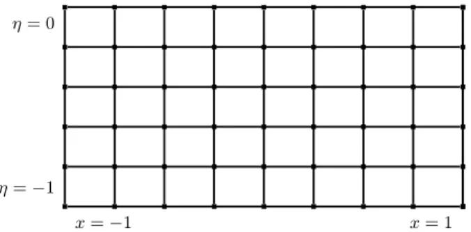
In our investigations all ingredients of the system are assumed to be homogeneous in one lateral direction so that we may in fact restrict the analysis to a cross section of the device. Denoting by ˜x and ˜z the horizontal and vertical direction, respectively, we consider the ground plate to be located at height ˜_{z = −h and the undeflected membrane at ˜z = 0, both having the length 2l. Moreover,} the length 2l of the device is assumed to be large compared to the gap size h of the undeformed configuration, which means that we are in the regime of a small aspect ratio ε = h

l ⌧ 1. x = −1 z = −1 x = 1 z = 0 = (1 + z)f = (1 + z)f = 0 = f u(t, x) Ω (u)

Figure 2.1: Cross section of the investigated idealised MEMS device.

An application of a voltage V to the conducting film on the membrane, such that the grounded plate and the membrane are at different electric potentials, induces a deformation of the elastic membrane assumed to be only in ˜z-direction. We denote the deformation at time ˜_{t ≥ 0 and position} ˜

x 2 L := (−l, l) by ˜u = ˜u(˜t, ˜x). The second quantity of general interest, the electrostatic potential 5

(19)

Chapter 2. The Modelling 6

at time ˜t ≥ 0 and a certain position (˜x, ˜z) in the region between the ground plate and the elastic membrane is denoted by ˜ψ = ˜ψ(˜t, ˜x, ˜z). It is worthwhile to mention again that the shape of this region changes with time as the membrane deflects with time. Finally we denote the permittivity profile of the membrane by f = f!˜x, ˜u(˜t, ˜x)"

.

2.1 | A Nonlinear Elasticity Model

For the nonce the time variable ˜t appears as a parameter, whence it is temporarily suppressed in the notation.

Governing Equations for the Electrostatic Potential. Pursuant to Gauß’ law of electrodynamics the electrostatic potential is harmonic in the region

˜

Ω(˜_{u) := {(˜x, ˜z); −l < ˜x < l, −h < ˜z < ˜u(˜x)}}

between the rigid ground plate and the membrane, that is ˜

ψ˜x˜x+ ˜ψz ˜˜z= 0, (˜x, ˜z) 2 ˜Ω(˜u).

Furthermore, the fixed plate at ˜_{z = −h is grounded, i.e. at zero potential, whereas the membrane} is at potential V f!˜x, ˜u(˜x)"

. These boundary conditions are expressed by the equations ˜

ψ(˜_{x, −h) = 0,} ψ! ˜˜ x, ˜u(˜x)" = V f!˜x, ˜u(˜x)", _{x 2 L.}˜

Governing Equations for the Membrane’s Deformation. By means of nonlinear elasticity theory we first derive the governing equations for the case of static plate defor-mations under the hypotheses of Love–Kirchhoff. In particular this includes the assumption that vectors normal to the middle surface remain normal to the middle surface after deformation. We refer the reader for instance to [8] for a detailed view on these hypotheses. Finally we assume the elastic plate to be of infinitely small thickness which reduces the more general model for plate de-formations to one describing dede-formations of elastic membranes. If no ambiguity is to be feared we use both expressions suitably.

The total potential energy Epof the configuration, which is generated due to the deformation of the

(20)

7 2.1. A Nonlinear Elasticity Model

electrostatic energy Ee, i.e. it holds

Ep(˜u) = Es(˜u) + Eb(˜u) + Ee(˜u).

Denoting by τ > 0 the tension constant of the plate, the stretching energy is given by

Es(˜u) = τ Z l −l ✓q 1 +! ˜ux˜(˜x)"2− 1 ◆ d˜x. (2.1)

The integral describes the variation of the plate’s length from 2l, i.e. from the situation in which deformation is absent.

The likewise involved bending energy is proportional to the L2-norm of the plate’s curvature. More

precisely, it is given by Eb(˜u) = b 2 Z l −l ∂x ˜ ux˜(˜x) p1 + (˜ux˜(˜x))2 !!2 p1 + (˜ux˜(˜x))2d˜x,

where the coefficient b, describing the flexural rigidity of the plate, is defined as

b = 2α

3_Y

3(1 − ν)2.

The parameters in this ratio denote the thickness α of the plate, the Young modulus Y and the Poisson ratio ν.

Finally, the electrostatic energy is given by

Ee(˜u) = −ε0 2 Z l −l Z u(˜˜x) −h ⇣ r ˜ψ(˜x, ˜z)⌘2d˜z d˜_{x = −}ε0 2 Z ˜ Ω(˜u) ⇣ r ˜ψ(˜x, ˜z)⌘2d(˜x, ˜z),

with ε0 being the permittivity of free space. The variation of Ee corresponds to the work of the

force on the elastic plate that is induced by the electric field with potential ˜ψ(˜x, ˜z).

Consequently, the total potential energy of the system is given by

Ep(˜u) = τ Z l −l ⇣p 1 + (˜ux˜(˜x))2− 1 ⌘ d˜x + b 2 Z l −l ∂x˜ ˜ u˜x(˜x) p1 + (˜ux˜(˜x))2 !!2 p1 + (˜ux˜(˜x))2d˜x −ε₂0 Z ˜ Ω(˜u) ⇣ r ˜ψ(˜x, ˜z)⌘2d(˜x, ˜z).

(21)

Derivation of the Euler-Lagrange Equation. Due to Hamilton’s principle of least action the partial differential equation describing the dynamics of the plate’s deformation is the Euler–Lagrange equation which is obtained by minimising a suitable energy functional.

The time dependent part of the problem is considered in a second step, whereas in a first step we derive the Euler–Lagrange equation in terms of static deflections. To this end we define the Lagrangian L : L ⇥ W24(L) −! R by L(˜x, ˜u) = − τ⇣p1 + (˜ux˜)2− 1 ⌘ −₂b∂x˜ u˜x˜ p1 + (˜ux˜)2 !2 p1 + (˜ux˜)2 +ε0 2 Z u˜ −h ⇣ ˜_ψ_x_˜_(˜_{x, ˜}_z)⌘2 +⇣ ˜ψz˜(˜x, ˜z) ⌘2 d˜z = − τ⇣p1 + (˜ux˜)2− 1 ⌘ −₂b_{(1 + (˜}u˜_ux˜˜x ˜ x)2)5/2 +ε0 2 Z ˜u −h ⇣ ˜_ψ_x_˜_(˜_{x, ˜}_z)⌘2 +⇣ ˜ψz˜(˜x, ˜z) ⌘2 d˜z

and minimise the according energy functional Z l

−lL(˜x, ˜u) d˜x

(2.2)

by means of calculus of variations. The problem of minimising an integral over an infinite dimen-sional function space is then treated as the problem of minimising a function of a single real-valued variable.1

In order to accomplish the latter problem assume that ˜u = ˜u(˜x) is the current minimiser of (2.2), satisfying

˜

u 2 W2,D4 (L), u(˜˜ x) > −h, x 2 [−l, l].˜ (2.3)

Then, given σ 2 R and a function v 2 C1

c (L), we introduce the notation

w(σ)(˜x) := ˜u(˜x) + σv(˜x), _{x 2 [−l, l],}˜

and derive the necessary condition for ˜u being a minimiser of (2.2) by computing the first variation

δEp(˜u; v) = d dσEp(˜u + σv)|σ=0= δ ⇣ Es(˜u; v) + Eb(˜u; v) + Ee(˜u; v) ⌘ |σ=0 (2.4) 1

In physics and engineering it is common to consider regularity assumptions as physically given and thus to presume the validity of the Euler–Lagrange equations. Mathematically speaking we therefore just verify the necessary condition for the existence of an extremum of the functional.

(22)

and finally checking the condition δEp(˜u; v) = 0. For the stretching term one obtains

d dσEs(˜u + σv) = d dσ ✓ τ Z l −l p1 + (w˜x)2− 1 d˜x ◆ = τ Z l −l ˜ ux˜vx˜+ σ(vx˜)2 p1 + (˜ux˜)2+ 2σ ˜u˜xvx˜+ σ2(vx˜)2 d˜x

and therefore, using the fact that v is compactly supported in the interval L,

δEs(˜u; v) = τ Z l −l ˜ ux˜vx˜ p1 + (˜ux˜)2 = −τ Z l −l v∂x˜ ˜ ux˜ p1 + (˜ux˜)2 ! d˜x. (2.5)

For the bending term, note that

∂˜x wx˜ p1 + (wx˜)2 ! = w˜x˜x (1 + ( ˜w˜x)2)3/2 ,

whence we may write

d dσEb(˜u + σv) = d dσ 0 @ b 2 Z l −l ∂x˜ wx˜ p1 + (wx˜)2 !!2 p1 + (wx˜)2d˜x 1 A = d dσ ✓ b 2 Z l −l (wx˜˜x)2 (1 + (wx˜)2)5/2 d˜x ◆ = b Z l −l (˜ux˜˜x+ σvx˜˜x)vx˜˜x (1 + (˜ux˜)2+ 2σ ˜u˜xvx˜+ σ2(v˜x)2)5/2 d˜_{x −}5b 2 Z l −l ! ˜u˜xvx˜+ σ(vx˜)2"! ˜u˜x˜x+ σ(vx˜˜x)"2 !1 + ˜u2 ˜ x+ 2σ ˜ux˜vx˜+ σ2(vx˜)2 "7/2 d˜x and again using that v(±l) = 0 we obtain

δEb(˜u; v) = b Z l −l ˜ ux˜˜x (1 + (˜ux˜)2)5/2 v˜x˜xd˜x − 5b 2 Z l −l ˜ ux˜(˜u˜x˜x)2 (1 + (˜u˜x)2)7/2 vx˜d˜x = b Z l −l ∂2_˜_x ✓ ˜ u˜x˜x (1 + (˜ux˜)2)5/2 ◆ v d˜x +5b 2 Z l −l ∂x˜ ✓ ˜ ux˜(˜ux˜˜x)2 (1 + (˜u˜x)2)7/2 ◆ v d˜x. (2.6)

It finally remains to take the electrostatic energy into account and to calculate δEe(˜u + σv). In the

sequel this is done by an application of the transport theorem, c.f. [4, XII, Theorem 2.11] or [28, Theorem 5.2.2] for instance. To this end, given σ 2 R, v 2 C1

c (L) and w(σ)(˜x) = ˜u(˜x) + σv(˜x)

as above, we pick σ0 > 0 such that the choice of ˜u as in (2.3) implies that w(σ)(˜x) > −h for all

˜

x 2 [−l, l] and all σ 2 [−σ0, σ0] and such that we may introduce the well-defined and connected

open set

˜

Ωσ := {(˜x, ˜z) 2 L ⇥ (−h, 1); −h < ˜z < w(σ)(˜x)} , σ 2 [−σ0, σ0].

In addition, there exists a representation ˜

(23)

of ˜Ωσ via the (global) diffeomorphism

φ(σ; ˜x, ˜z) := ✓ ˜ x, ˜z + σv(˜x) h + ˜z h + ˜u(˜x) ◆ , (˜x, ˜_{z) 2 ˜}Ω(˜u) = ˜Ω0.

In order to be able to handle the electrostatic energy with a variational approach it is necessary to investigate the problem for ˜ψ corresponding to the variation w of the minimiser ˜u in direction v. For this purpose denote by ˜ψ(σ; ˜_{u, v) 2 W}2

2( ˜Ωσ) the solution to ˜ ψx˜˜x(σ; ˜u, v) + ˜ψz ˜˜z(σ; ˜u, v) = 0, (˜x, ˜z) 2 ˜Ωσ, (2.7) ˜ ψ(σ; ˜u, v) = h + ˜z h + w(σ)(˜x)V f! ˜x, w(σ)(˜x)", (˜x, ˜z) 2 ∂ ˜Ωσ. (2.8) Moreover, we introduce the velocity V of the path { ˜ψ(σ; ˜_{u, v); σ 2 (−σ}0, σ0)}, defined as2

V := _dσd ψ(σ; ˜_{u, v)|}σ=0, (˜x, ˜z) 2 ˜Ω(˜u). (2.9)

and show that also V satisfies (2.7)–(2.8) in the limit σ = 0. To this end, observe that (2.7) is equivalent to3 ˜ ψ˜x˜x ✓ σ; ˜x, ˜z + σv(˜x) h + ˜z h + ˜u(˜x) ◆ + ˜ψz ˜˜z ✓ σ; ˜x, ˜z + σv(˜x) h + ˜z h + ˜u(˜x) ◆ = 0, (˜x, ˜_{z) 2 ˜}Ω(˜u),

whence a differentiation of this equation with respect to σ yields

˜ ψ˜x˜xσ ✓ σ; ˜x, ˜z + σv(˜x) h + ˜z h + ˜u(˜x) ◆ + ˜ψ˜x˜x˜z ✓ σ; ˜x, ˜z + σv(˜x) h + ˜z h + ˜u(˜x) ◆ v(˜x) h + ˜z h + ˜u(˜x) + ˜ψ˜z ˜zσ ✓ σ; ˜x, ˜z + σv(˜x) h + ˜z h + ˜u(˜x) ◆ + ˜ψz ˜˜z ˜z ✓ σ; ˜x, ˜z + σv(˜x) h + ˜z h + ˜u(˜x) ◆ v(˜x) h + ˜z h + ˜u(˜x)= 0, (2.10)

for all (˜x, ˜_{z) 2 ˜}Ω(˜_{u). Then, letting σ ! 0 in (2.10), we first find that}

V˜x˜x(˜x, ˜z) + Vz ˜˜z(˜x, ˜z) + v(˜x) h + ˜z h + ˜u(˜x)⇣ ˜ψ˜x˜x˜z(˜x, ˜z) + ˜ψ˜z ˜z ˜z(˜x, ˜z) ⌘ = 0, (˜x, ˜_{z) 2 ˜}Ω(˜u), whence by (2.7) V˜x˜x(˜x, ˜z) + V˜z ˜z(˜x, ˜z) = 0, (˜x, ˜z) 2 ˜Ω(˜u). 2

Note that in fact V is a function of the variables ˜x and ˜z in the sense that V(˜x, ˜z) = d

dσ (σ; ˜u, v)|σ=0(˜x, ˜z).

3

In fact ˜ !σ; ˜u, v" is a function of the variables ˜x and ˜z. For the sake of simplicity we suppress the dependence of ˜

(24)

In addition, one can infer from the boundary condition (2.8) that

˜ ψ ✓ σ; ˜x, ˜z + σv(˜x) h + ˜z h + ˜u(˜x) ◆ = h + ˜z

h + ˜u(˜x)V f! ˜x, ˜u(˜x) + σv(˜x)", (˜x, ˜z) 2 ∂ ˜Ω(˜u), and differentiating this identity with respect to σ yields

˜ ψσ ✓ σ; ˜x, ˜z + σv(˜x) h + ˜z h + ˜u(˜x) ◆ + ˜ψ˜z ✓ σ; ˜x, ˜z + σv(˜x) h + ˜z h + ˜u(˜x) ◆ v(˜x) h + ˜z h + ˜u(˜x) = h + ˜z h + ˜u(˜x)V fu˜! ˜x, ˜u(˜x) + σv(˜x)"v(˜x) for (˜x, ˜_{z) 2 ∂ ˜}Ω(˜_{u). Finally, as σ ! 0 we find that}

V(˜x, ˜z) = v(˜x)_{h + ˜}h + ˜_u(˜z_x)⇣V fu˜! ˜x, ˜u(˜x)" − ˜ψz˜(˜x, ˜z)

⌘

, (˜x, ˜_{z) 2 ∂ ˜}Ω(˜u). (2.11)

Since v 2 C1

c (L) and h + ˜z = 0 for ˜z = −h, one may in particular extract from equation (2.11) the

identities

V(±l, ˜z) = 0, _{z 2 (−h, 0),}˜

V(˜x, −h) = 0, _{x 2 L,}˜ (2.12) V(˜x, ˜u(˜x)) = v(˜x)⇣V fu˜! ˜x, ˜u(˜x)" − ˜ψz˜! ˜x, ˜u(˜x)"

⌘

, _{x 2 L.}˜

Having this preliminary knowledge at hand, we are finally prepared to consider the energy

Ee(˜u + σv) = − ε0 2 Z ˜ Ωσ !_˜ ψ˜x(σ; ˜x, ˜z)"2+!ψ˜z˜(σ; ˜x, ˜z)"2d(˜x, ˜z)

or, more precisely, its derivative with respect to σ at σ = 0. Firstly, invoking [28, Thm. 5.2.2] yields the identity δEe(˜u; v) = − ε0 Z ˜ Ω(˜u) ˜ ψx˜(˜x, ˜z)V˜x(˜x, ˜z) + ˜ψz˜(˜x, ˜z)Vz˜(˜x, ˜z) d(˜x, ˜z) − ε0 Z ˜ Ω(˜u) div ! ˜ψx˜(˜x, ˜z) "2 +!_˜ ψz˜(˜x, ˜z)"2 2 φσ(0, ˜x, ˜z) ! d(˜x, ˜z) (2.13)

and using (2.7) one can readily see that

div⇣_V⇣ ˜ψ˜x, ˜ψ˜z ⌘⌘ = Vx˜ψ˜˜x+ V ˜ψx˜˜x+ Vz˜ψ˜z˜+ V ˜ψz ˜˜z = Vx˜ψ˜˜x+ Vz˜ψ˜˜z+ V⇣ ˜ψx˜˜x+ ˜ψz ˜˜z ⌘ = Vx˜ψ˜˜x+ Vz˜ψ˜˜z (2.14)

(25)

holds true for all (˜x, ˜_{z) 2 ˜}Ω(˜u). Then, fusing the findings (2.13) and (2.14) leads to the equation

δEe(˜u; v) = − ε0 Z ˜ Ω(˜u) div⇣_{V(˜x, ˜z)}⇣ ˜ψ˜x(˜x, ˜z), ˜ψz˜(˜x, ˜z) ⌘⌘ d(˜x, ˜z) − ε0 Z ˜ Ω(˜u) div ! ˜ψx˜(˜x, ˜z) "2 +!_˜ ψ˜z(˜x, ˜z)"2 2 φσ(0, ˜x, ˜z) ! d(˜x, ˜z).

Allowing for the identity

φσ(0; ˜x, ˜z) = ✓ 0, v(˜x) h + ˜z h + ˜u(˜x) ◆ , (˜x, ˜_{z) 2 ˜}Ω(˜u),

an application of the Green–Riemann integration theorem reveals

δEe(˜u; v) = − ε0 Z ∂ ˜Ω(˜u)V(˜x, ˜z) ˜ ψ˜x(˜x, ˜z) d˜z + ε0 Z ∂ ˜Ω(˜u)V(˜x, ˜z) ˜ ψz˜(˜x, ˜z) d˜z +ε0 2 Z ∂ ˜Ω(˜u) v(˜x) h + ˜z h + ˜u(˜x) ⇣_! ˜ ψ˜x(˜x, ˜z)"2+!ψ˜z˜(˜x, ˜z)"2 ⌘ d˜x.

Then, exploiting the relations v(±l) = 0, h + ˜z = 0 for ˜z = −h, and the boundary conditions (2.12) for V, the above integrals vanish at the lateral boundaries and on the ground plate at ˜z = −h, whereby we obtain

δEe(˜u; v) = ε0V

Z l

−l

v(˜x)fu˜! ˜x, ˜u(˜x)"⇣ ˜ψx˜! ˜x, ˜u(˜x)" ˜u˜x(˜x) − ˜ψz˜! ˜x, ˜u(˜x)"

⌘ d˜x

− ε0

Z l

−l

v(˜x)⇣ ˜ψx˜! ˜x, ˜u(˜x)"ψ˜˜z! ˜x, ˜u(˜x)" ˜u˜x(˜x) −!ψ˜z˜(˜x, ˜u(˜x))"2

⌘ d˜x −ε₂0 Z l −l v(˜x)⇣!˜ ψ˜x(˜x, ˜u(˜x))"2+!ψ˜z˜(˜x, ˜u(˜x))"2 ⌘ d˜x.

From the boundary condition ˜ψ! ˜x, ˜u(˜x)" = V f!˜x, ˜u(˜x)", ˜_{x 2 L, we may deduce the equality} ˜ ψ˜z! ˜x, ˜u(˜x)" ˜ux˜(˜x) = V ⇣ fx˜! ˜x, ˜u(˜x)" + fu˜! ˜x, ˜u(˜x)" ˜u˜x(˜x) ⌘ − ˜ψx˜! ˜x, ˜u(˜x)",

and it follows that

δEe(˜u; v) = ε0V

Z l

−l

v(˜x)fu˜! ˜x, ˜u(˜x)"⇣ ˜ψx˜! ˜x, ˜u(˜x)" ˜ux˜(˜x) − ˜ψz˜! ˜x, ˜u(˜x)"

⌘ d˜x − ε0V Z l −l v(˜x) ˜ψx˜! ˜x, ˜u(˜x)" ⇣ fx˜! ˜x, ˜u(˜x)" + fu˜! ˜x, ˜u(˜x)" ˜ux˜(˜x) ⌘ d˜x +ε0 2 Z l −l v(˜x)⇣!˜ ψ˜x(˜x, ˜u(˜x))"2+!ψ˜z˜(˜x, u(˜x))"2 ⌘ d˜x.

(26)

This equation may finally be rewritten as

δEe(˜u; v) = ε0 2 Z l −l v(˜x)⇣!_˜ ψ˜x(˜x, ˜u(˜x))"2+!ψ˜z˜(˜x, ˜u(˜x))"2 ⌘ d˜x − ε0V Z l −l

v(˜x)⇣ ˜ψx˜! ˜x, ˜u(˜x)"fx˜! ˜x, ˜u(˜x)" + ˜ψ˜z! ˜x, ˜u(˜x)"fu˜! ˜x, ˜u(˜x)"

⌘ d˜x.

(2.15)

Recalling (2.4) as well as the equality

δEp(˜u; v) = δ

⇣

Es(˜u; v) + Eb(˜u; v) + Ee(˜u; v)

⌘ = 0

as a necessary condition for ˜u being a minimiser of the energy functional (2.2), we may see by (2.5), (2.6) and (2.15) that this is satisfied for all suitable functions v, if and only if ˜u complies with the Euler–Lagrange equation 0 = τ ∂˜x ˜ ux˜ p1 + (˜u˜x)2 ! − b∂2˜x ✓ _u_˜ ˜ x˜x (1 + (˜ux˜)2)5/2 ◆ −5b₂∂x˜ ✓ _u_˜ ˜ x(˜u˜x˜x)2 (1 + (˜u˜x)2)7/2 ◆ −ε₂0⇣!_˜ ψx˜(˜x, ˜u(˜x))"2+!ψ˜z˜(˜x, ˜u(˜x))"2 ⌘

+ ε0V ⇣ ˜ψx˜! ˜x, ˜u(˜x)"f˜x! ˜x, ˜u(˜x)" + ˜ψz˜! ˜x, ˜u(˜x)"fu˜! ˜x, ˜u(˜x)"

⌘ .

Heretofore, static deflections of the elastic plate are discussed and it remains to take the dynamics into account. This means that from now on the time variable ˜t explicitly returns to the notation. More precisely, denoting by ρ the mass density per unit volume of the plate and recalling that α denotes its thickness, due to Newton’s Second Law the sum of all forces is equal to ρα˜u˜t˜t(˜t, ˜x) and

we get ρα˜u˜t˜t(˜t, ˜x) − τ∂x˜ ˜ ux˜ p1 + (˜ux˜)2 ! + b∂x2˜ ✓ _u_˜ ˜ x˜x (1 + (˜u˜x)2)5/2 ◆ +5b 2∂x˜ ✓ _u_˜ ˜ x(˜ux˜˜x)2 (1 + (˜ux˜)2)7/2 ◆ = −ε₂0⇣!_˜ ψx˜(˜x, ˜u(˜x))"2+!ψ˜z˜(˜x, ˜u(˜x))"2 ⌘

⌘ .

Lastly, the superposition of the elastic and electrostatic forces is combined with a damping force −a˜u˜t which is linearly proportional to the velocity ˜u˜t with damping constant a. That is, we obtain

ρα˜u˜t˜t(˜t, ˜x) + a˜u˜t− τ∂x˜ ˜ ux˜ p1 + (˜ux˜)2 ! + b∂_x2_˜ ✓ ˜ ux˜˜x (1 + (˜ux˜)2)5/2 ◆ +5b 2∂˜x ✓ ˜ ux˜(˜ux˜˜x)2 (1 + (˜ux˜)2)7/2 ◆ = −ε₂0⇣!_˜ ψx˜(˜x, ˜u(˜x))"2+!ψ˜z˜(˜x, ˜u(˜x))"2 ⌘

⌘ .

Fusing the above considerations we end up with the following coupled system of partial differential equations. The elliptic free boundary value problem for the electrostatic potential in the region determined by the grounded plate at ˜_{z = −h and the membrane at ˜z = ˜u(˜t, ˜x), both of length 2l,}

(27)

Chapter 2. The Modelling 14 reads ˜ ψ˜x˜x+ ˜ψz ˜˜z= 0, t > 0, (˜˜ x, ˜z) 2 ˜Ω(˜u), (2.16) ˜ ψ(˜t, ˜x, ˜z) = h + ˜z

h + ˜u(˜t, ˜x)f! ˜x, ˜u(˜t, ˜x)", ˜t > 0, (˜x, ˜z) 2 ∂ ˜Ω(˜u), (2.17) where the conditions ˜ψ = 0 and ˜ψ = V f! ˜x, ˜u(˜t, ˜x)"

on the ground plate and the membrane, respec-tively, are continuously extended to the lateral boundaries (±l, ˜z), ˜z 2 (−h, 0). The dynamics of the deflection ˜u is thus described by the fourth-order equation

ρα˜u˜t˜t+ a˜u˜t+ ˜A1(˜u) = − ε0 2 ⇣ !˜ ψx˜(˜x, ˜u(˜x))"2+!ψ˜˜z(˜x, ˜u(˜x))"2 ⌘

+ ε0V⇣ ˜ψx˜! ˜x, ˜u(˜x)"fx˜! ˜x, ˜u(˜x)" + ˜ψz˜! ˜x, ˜u(˜x)"fu˜! ˜x, ˜u(˜x)"

⌘ ,

(2.18)

where ˜A1(˜u) is the quasilinear fourth-order differential operator defined by

˜ A1(˜u) := −τ∂x˜ ˜ ux˜ p1 + (˜ux˜)2 ! + b∂x2˜ ✓ _u_˜ ˜ x˜x (1 + (˜ux˜)2)5/2 ◆ +5b 2∂x˜ ✓ _u_˜ ˜ x(˜ux˜˜x)2 (1 + (˜ux˜)2)7/2 ◆ .

Furthermore, we assume the membrane to be clamped at its boundary (±l, 0) and to have a certain initial deflection ˜u⇤(˜x) at time ˜t = 0. This is expressed by the clamped boundary conditions

˜

u(˜_{t, ±l) = ˜u}˜x(˜t, ±l) = 0, ˜t > 0,

and the initial conditions

˜

u(0, ˜x) = ˜u⇤(˜x), u˜t˜(0, ˜x) = ˜u⇤⇤(˜x), x 2 L,˜

respectively. 2.1.1 Remark

We briefly discuss two variants of the above modelling by distinguishing energy conserving and energy dissipating systems. Whereas the first occurs when damping effects are neglected, the latter corresponds to the case of no inertial effects.

(1) We assume to be in an energy conserving Hamiltonian regime in which damping is not taken into account. The total energy of the system is defined as the pointwise difference of kinetic energy Ek and potential energy Ep. The kinetic energy at any instant in time is described by

the functional Ek(˜u) = ρα 2 Z l −l ! ˜u˜t "2 d˜x.

(28)

to minimise the action of the system, i.e. the double integral Z t2

t1

Z l

−lL(˜t, ˜x, ˜u) d˜x d˜t,

where the Lagrangian L is now given by4

L : (t1, t2) ⇥ L ⇥ W22,4!(t1, t2) ⇥ L" ! R, L(˜t, ˜x, ˜u) = ρα₂ u˜2_˜_t _{− τ}⇣p1 + (˜ux˜)2− 1 ⌘ −₂b_{(1 + (˜}u˜_ux˜˜x ˜ x)2)5/2 +ε0 2 Z ˜u −h ⇣ ˜_ψ_x_˜_(˜_{x, ˜}_z)⌘2 +⇣ ˜ψz˜(˜x, ˜z) ⌘2 d˜z,

and the corresponding Euler–Lagrange equation, obtained by a straightforward adaption of the above calculations, reads

ρα˜u˜t˜t+ ˜A1(˜u) = − ε0 2 ⇣ !˜ ψ˜x(˜x, ˜u(˜x))"2+!ψ˜z˜(˜x, ˜u(˜x))"2 ⌘

+ ε0V ⇣ ˜ψ˜x! ˜x, ˜u(˜x)"fx˜! ˜x, ˜u(˜x)" + ˜ψz˜! ˜x, ˜u(˜x)"fu˜! ˜x, ˜u(˜x)"

⌘ .

(2) Being in the energy dissipating regime where inertial effects are neglected, we shall see in the following that the corresponding evolution equation may formally be perceived as a gradient flow system.

(i) Let H be a Hilbert space over R with inner product (·, ·)H and let E 2 C(H, R) denote

a continuous functional on H. Given v 2 H, assume that

δE(v; w) := d

dσE(v + σw)|σ=0

exists in H for all w 2 H. Under this hypothesis assume in addition that there is a z(v) 2 H such that

!z(v), w"_H = δE(v; w), _{w 2 H.}

Note that z(v) is uniquely determined if it exists. We call z(v) the generalised gradient of E at v and use the notation

rE(v) := z(v). If E 2 C1(H, R) then rE(v) exists for all v 2 H with

DE(v)w =_{!rE(v), w"}_H, _{w 2 H.}

(ii) Given T > 0, consider v 2 C1_{!(0, T ), H" and assume that rE!v(t)" exists in H for all}

4

(29)

t 2 (0, T ). If v complies with the equation

v0_{(t) = −rE}!v(t)", _{t 2 (0, T ),} (2.19) then we say that v is a solution to the gradient flow system associated to E on (0, T ). (iii) Suppose that E is contained in C1_{(H, R) and v 2 C}1_{!(0, T ), H" is a solution to (2.19)}

on (0, T ). Then E_{!v(t)" is decreasing on (0, T ). Indeed E!v(·)" is differentiable on (0, T )} and the chain rule yields

d dtE!v(t)" = !rE(v(t)), v 0_(t)" H= −krE!v(t)"k 2 H, t 2 (0, T ). (2.20)

Interpreting E as an energy the last equation reveals the energy dissipation of the system. Moreover, if the path v(t) avoids any critical point of E the dissipation is strict.

(iv) Taking H = L2(L) and E(˜u) = Ep(˜u) with ˜u 2 W2,D4 (L) we deduce from (2.5), (2.6) and

(2.15) that formally rEp(˜u) = −A1(˜u) −ε0 2 ⇣_! ˜ ψx˜(˜x, ˜u(˜x))"2+!ψ˜˜z(˜x, ˜u(˜x))"2 ⌘

+ ε0V ⇣ ˜ψ˜x! ˜x, ˜u(˜x)"fx˜! ˜x, ˜u(˜x)" + ˜ψz˜! ˜x, ˜u(˜x)"fu˜! ˜x, ˜u(˜x)"

⌘ .

This means that if ρ = 0 and a = 1 equation (2.18) may be perceived as the gradient flow system associated to Ep in L2(L).

Scaling – Introduction of Dimensionless Variables. Now dimensionless variables are introduced and the above terms and equations are rewritten in dimensionless form. To that effect, the electrostatic potential is scaled with the applied voltage,

ψ = ψ˜ V, the time is scaled with a damping timescale of the system,

t = τ al2˜t,

and the variables ˜x and ˜z as well as ˜u are scaled with the length l and the gap size h of the undeflected configuration, respectively, x = x˜ l, z = ˜ z h, u = ˜ u h. (2.21)

(30)

problem for the electrostatic potential thus reads

ε2ψxx+ ψzz = 0, t > 0, (x, z) 2 Ω(u(t)),

ψ(t, x, z) = 1 + z

1 + u(t, x)f!x, u(t, x)", t > 0, (x, z) 2 ∂Ω(u(t)), where the region Ω(u(t)) is now given by

Ω(u(t)) = {(x, z) 2 (−1, 1) ⇥ (−1, 1); −1 < z < u(t, x)} .

In dimensionless form the evolution of the membrane’s deflection is specified by the equation

ραhτ 2 a2_l4utt+ hτ l2 ut+ A1(u) = − ε0V2 2 ✓ 1 l2!ψx(x, u(x)) "2 + 1 h2!ψz(x, u(x)) "2 ◆ + ε0V2 ✓ 1 l2ψx!x, u(x)"fx!x, u(x)" + 1 h2ψz!x, u(x)"fu!x, u(x)" ◆ , (2.22) with A1(u) given by

A1(u) = − τ ε l ∂x ux p1 + ε2_(u x)2 ! +bε l3∂ 2 x ✓ uxx (1 + ε2_(u x)2)5/2 ◆ +5bε 3 2l3 ∂x ✓ ux(uxx)2 (1 + ε2_(u x)2)7/2 ◆ .

Multiplying (2.22) by l2_{/hτ and using the definition of ε then leads to the equation}

ρατ a2_l2utt+ ut+ A(u) = − ε0V2 2ε2_hτ ⇣ ε2!ψx(x, u(x))"2+!ψz(x, u(x))"2 ⌘ + ε0V ε2_hτ ⇣

ε2ψx!x, u(x)"fx!x, u(x)" + ψz!x, u(x)"fu!x, u(x)"

⌘ , with the rescaled quasilinear fourth-order differential operator

A(u) := l 2 hτA1(u) = −∂x ux p1 + ε2_(u_x₎2 ! + b l2_τ∂ 2 x ✓ uxx (1 + ε2_(u x)2)5/2 ◆ +5bε 2 2l2_τ∂x ✓ ux(uxx)2 (1 + ε2_(u x)2)7/2 ◆ .

Lastly, by introduction of the parameters

γ := p_ρατ al , β := b τ l2, λ = λ(ε) := ε0V2 2ε2_hτ,

(31)

Chapter 2. The Modelling 18 evolution equation γ2utt+ ut+ A(u) = −λ ⇣ ε2!ψx(x, u(x))"2+!ψz(x, u(x))"2 ⌘

+ 2λ⇣ε2ψx!x, u(x)"fx!x, u(x)" + ψz!x, u(x)"fu!x, u(x)"

⌘ , with A(u) = −∂x ux p1 + ε2_(u x)2 ! + β∂_x2 ✓ _u xx (1 + ε2_(u x)2)5/2 ◆ +5 2βε 2_∂ x ✓ _u x(uxx)2 (1 + ε2_(u x)2)7/2 ◆

and the according boundary and initial conditions

u(t, ±1) = ux(t, ±1) = 0, t > 0,

u(0, x) = u⇤(x), ut(0, x) = u⇤⇤(x), x 2 (−1, 1).

Here, γ is the systems quality factor5_{, β measures the relative importance of tension and rigidity}

and λ is a ratio of a reference electrostatic force to a reference elastic force. It is proportional to the square of the applied voltage and serves as a tuning parameter for the system.

2.2 | A Simplified Linear Elasticity Model

In the previous section, a general model for the dynamic behaviour of an electrostatically actuated MEMS device has been derived by means of nonlinear elasticity theory. Allowing also for large deflections of the membrane, it is the characteristic of the governing elasticity terms to be nonlinear. However, in many engineering applications it is reasonable to only require the device to feature small membrane deflections and thus to restrict the mathematical investigations to a linear elasticity model. It is the purpose of this section to derive the analgon of the above model by means of linear elasticity theory.

Starting from the unscaled regime, in a first step, we assume (˜ux˜)2 to be small, i.e. (˜ux˜)2⌧ 1, and

consider the Taylor series expansion

p1 + (˜ux˜)2' 1 +

1 2(˜ux˜)

2_{+ . . .}

of the term p1 + (˜ux˜)2 around (˜ux˜)2 = 0, ignoring all but the first two terms.6 The linearised

5

Recall that γ = p⇢↵⌧ /al is a measure for the damping of an oscillating system. Small values γ refer to strongly damped systems and thus indicate a large rate of decay of oscillations.

6

Note that the constant first term in the Taylor series expansion just voids the constant length in the stretching energy, whence we include the second term (˜u˜x)2/2 as well.

(32)

19 2.2. A Simplified Linear Elasticity Model

stretching energy may then be written as

Es(˜u) = τ 2 Z l −l (˜ux˜! ˜x)"2d˜x.

As before, given σ 2 R and a function v 2 C1

c (L), we introduce for ˜x 2 [−l, l] the variation

w(σ)(˜x) = ˜u(˜x) + σv(˜x) of ˜u(˜x) in the direction of v. We then find that d dσEs(˜u + σv) = d dσ ✓ τ 2 Z l −l (w˜x)2d˜x ◆ = τ Z l −l ˜ u˜xvx˜+ σ(vx˜)2d˜x

whence, using that v is compactly supported in L,

δEs(˜u; v) = τ Z l −l ˜ ux˜v˜xd˜x = −τ Z l −l ˜ ux˜˜xv d˜x.

We proceed similarly in order to obtain the a linearised version of the bending term. Again requiring (˜ux˜)2⌧ 1 to be small, we consider the Taylor series expansion

∂x˜ ˜ u˜x p1 + (˜ux˜)2 !!2 p1 + (˜ux˜)2= (˜ux˜˜x)2 (1 + (˜ux˜)2)5/2 ' (˜ux˜˜x )2+ . . .

around (˜ux˜)2= 0, whence the linearised bending energy reads

Eb(˜u) = b 2 Z l −l ! ˜ux˜˜x(˜x)"2d˜x.

Therefore, we find that d dσEb(˜u + σv) = d dσ ✓ b 2 Z l −l (w˜x˜x)2d˜x ◆ = b Z l −l ˜ u˜x˜xvx˜˜x+ σ(vx˜˜x)2d˜x

and thus finally

δEb(˜u; v) = b Z l −l ˜ ux˜˜xvx˜˜xd˜x = b Z l −l ˜ ux˜˜x˜x˜xv d˜x.

With the same scaling as above, the Euler–Lagrange equation in the regime of linear elasticity reads

γ2utt+ ut− uxx+ βuxxxx= −λ

⇣

ε2!ψx(x, u(x))"2+!ψz(x, u(x))"2

⌘

+ 2λ⇣ε2ψx!x, u(x)"fx!x, u(x)" + ψz!x, u(x)"fu!x, u(x)"

⌘ (2.23)

(33)

2.3 | The Mathematical Models Under Study

Based on the previous two sections, it is the purpose of the present one to give a brief overview of the different variants of the very general nonlinear and linear elasticity models, respectively, which reflect different physical assumptions, as they are adequate for different applications. Even if there are more variants conceivable, the presented elaboration is restricted to those models which are investigated more detailed in the subsequent chapters.

To this end, denoting by u = u(t, x), t > 0, x 2 I := (−1, 1), the membrane’s deformation, the elliptic problem governing the electrostatic potential of the system at any instant t ≥ 0 of time always reads

ψxx+ ψzz = 0, t > 0, (x, z) 2 Ω(u), (2.24)

ψ(t, x, z) = 1 + z

1 + u(t, x)f!x, u(t, x)", t > 0, (x, z) 2 ∂Ω(u), (2.25) where the region Ω(u(t)) between the rigid ground plate at z = −1 and the elastic membrane at z = u(t, x) at any instant of time is given by

Ω(u) = {(x, z) 2 (−1, 1) ⇥ (−1, 1); −1 < z < u(t, x)}.

Depending on the choice of the evolution equation for the membrane’s displacement, only the per-mittivity profile might vary, being either a function f = f(x), f = f!u(t, x)" or f = f!x, u(t, x)". In the above elliptic moving boundary value problem this does only influence the boundary condition accordingly.

The situation is more involved for the choice of an appropriate model describing the dynamics of the thin elastic plate’s displacement. Within the scope of both approaches – the linear and the nonlinear elasticity theory – in the following analysis we make two physical assumptions which have significant effects on the mathematical classification of the resulting equations.

First of all, we restrict the further investigations to viscosity-dominated systems, i.e. to a setting in which damping effects dominate over inertial effects. More precisely, this means that the parameter γ appearing in front of the inertial term is assumed to be very small, i.e.

γ = p_ρατ

al ⌧ 1, and thus that we ignore the inertial term γ2_u

ttin the equations. Note that the highest-order time

derivative thus appears in the shape of the damping term utwhich is of first order. This restriction

(34)

21 2.3. The Mathematical Models Under Study

behaviour of micro pumps [48] or micro grippers [49].

One may furthermore act on the assumption that membranes or infinitely thin plates do not resist bending, i.e. they have no flexural rigidity. This is the case if

b = 2α

3_Y

3(1 − ν)2 = 0 =) β =

b τ l2 = 0,

and thus the spatial higher-oder terms

β∂x2 ✓ _u xx (1 + ε2_(u x)2)5/2 ◆ +5 2βε 2_∂ x ✓ _u x(uxx)2 (1 + ε2_(u x)2)7/2 ◆ or βuxxxx,

in the nonlinear or linear elasticity regime, respectively, are eliminated. Deformations due to bending are thus neglected, which means that the governing equations are reduced from fourth-order to second-order (spatial) equations. Representatives for MEMS devices for which the suppression of bending effects is reasonable are certain micro pumps or the Grating Light Valve, respectively [45, p. 239].

Combining the above two physical assumptions we end up with a model influenced by stretching, damping and electrostatic forces. Note that those models are not admissible for all kinds of appli-cations, but that on the other hand there exist applications for which a negligence of inertial and bending effects is reasonable.

It finally remains to take different varying permittivity profiles into account. The simplest case of a constant permittivity f ⌘ 1 has extensively been studied in the recent time and is thus not a subject in the present study. It is rather the main objective of this thesis to consider the case in which the membrane exhibits a certain varying dielectric permittivity profile, itself depending either on the spatial variable x 2 I, the membrane’s displacement u = u(t, x), or even both. More precisely, the permittivity profile is given by a function of one of the three following types:

• [x 7! f(x)] : I ! R; • [u 7! f(u)] : (−1, 1) ! R;

• [(x, u) 7! f(x, u)] : I ⇥ (−1, 1) ! R.

Depending on the choice of the dielectric permittivity profile, also the right-hand side of the evolution equation differs. Denoting the right-hand side in any case by gε,λ(u), if f = f (x), it is given by

gε,λ(u) := −λ

⇣

ε2!ψx(x, u)"2+!ψz(x, u)"2

⌘

+ 2λε2ψx(x, u)f0(x), (2.26)

(35)

Chapter 2. The Modelling 22 reads gε,λ(u) := −λ ⇣ ε2!ψx(x, u)"2+!ψz(x, u)"2 ⌘ + 2λψz(x, u)f0(u), (2.27)

f0 _{denoting the derivative of f with respect to u, and finally in the case f = f(x, u) we have}

gε,λ(u) := −λ ⇣ ε2!ψx(x, u)"2+!ψz(x, u)"2 ⌘ + 2λ⇣ε2ψx(x, u)fx(x, u) + ψz(x, u)fu(x, u) ⌘ , (2.28)

fxand fu denoting the partial derivatives of f with respect to its first and second variable,

respec-tively.

Reviewing the above considerations as a whole, we end up with the quasilinear parabolic initial-boundary value problem

ut− ∂x ux p1 + ε2_(u x)2 ! = gε,λ(u) t > 0, x 2 I, (2.29) u(t, ±1) = 0, t > 0, (2.30) u(0, x) = u⇤(x), x 2 I, (2.31)

in the regime of nonlinear elasticity, whence in the linear elasticity setting the analogue problem is a semilinear parabolic initial-boundary value problem which reads

ut− uxx= gε,λ(u) t > 0, x 2 I, (2.32)

u(t, ±1) = 0, t > 0, (2.33) u(0, x) = u⇤(x), x 2 I, (2.34)

with a right-hand side according to the choice of the dielectric permittivity profile f.

2.3.1 Remark (1) Note that in both cases, (2.29)–(2.31) and (2.32)–(2.34), the evolution problem for the membrane’s displacement is strongly coupled to the elliptic moving boundary problem (2.24)–(2.25) in the following way. On the one hand the solution to the elliptic free boundary value problem is to be determined in the domain Ω(u(t)) which changes its shape with time as the membrane deflects with time. The coupling is thus observably in the boundary conditions for ψ. On the other hand, the right-hand side of the evolution equation for the membrane’s deformation u exhibits a nonlinear and nonlocal dependence of the gradient of the potential ψ.

(2) Observe that the above reasoning is formal in the sense that several regularity properties are used which are not verified rigorously, e.g.

(36)

23 2.3. The Mathematical Models Under Study

– _{the differentiability of the path {ψ(σ; u); σ 2 (−σ}0, σ0)} with respect to σ, c.f. (2.9),

– the additional spatial regularity of ψ used to derive (2.10)

(3) In the mathematical and numerical analysis in this thesis the main attention is devoted to the linear elasticity model (2.32)–(2.34) with the most general permittivity profile f = f (x, u), as far as possible. Nonetheless, the nonlinear elasticity model (2.29)–(2.31) is analysed precisely. It should be mentioned that for the latter model the presented results are partly based on joint works with Joachim Escher.

(37)

(38)

3 | Local Well-Posedness and Global

Existence

As a first aspect in the mathematical analysis of the coupled systems derived in Chapter 2 we address the questions of existence and uniqueness of solutions. Both when the membrane’s displacement is determined in the semilinear regime (2.32)–(2.34) as well as when it is described by the quasilinear problem (2.29)–(2.31), it turns out that the answers to those questions strongly depend on the applied voltage. More precisely, we show that the systems possess locally in time existing unique solutions for all arbitrarily large values λ of the applied voltage, and that solutions exist even globally in time, provided that the applied voltage does not exceed a certain critical value λ⇤.

Section 3.1 deals with the semilinear problem (2.32)–(2.34) arising from linear elasticity theory, whereas Section 3.2 is addressed to its quasilinear counterpart (2.29)–(2.31) arising from nonlinear elasticity theory.

3.1 | On the Semilinear Case

Based on the work [40] this section is devoted to results on local well-posedness and global existence of solutions to the coupled system of partial differential equations consisting of the semilinear parabolic initial boundary value problem

ut− uxx= −λ ⇣ ε2!ψx(x, u)"2+!ψz(x, u)"2 ⌘ + 2λ⇣ε2ψx(x, u)fx(x, u) + ψz(x, u)fu(x, u) ⌘ , _{t > 0, x 2 I,} (3.1) u(t, ±1) = 0, t > 0, (3.2) u(0, x) = u⇤(x), x 2 I, (3.3) 25

(39)

Chapter 3. Local Well-Posedness and Global Existence 26

describing the time evolution of the displacement u = u(t, x) of the membrane, and the elliptic free boundary value problem

ε2ψxx+ ψzz = 0, t > 0, (x, z) 2 Ω(u(t)), (3.4)

ψ(t, x, z) = 1 + z

1 + u(t, x)f!x, u(t, x)", t > 0, (x, z) 2 ∂Ω(u(t)), (3.5) characterising the electrostatic potential ψ = ψ(t, x, z) in the region

Ω(u(t)) = {(x, z) 2 (−1, 1) ⇥ (−1, 1); −1 < z < u(t, x)},

determined by the rigid ground plate at z = −1 and the elastic membrane at z = u(t, x). It is worthwhile to mention again the meaning of the two parameters ε and λ occurring in the above equations. The first one, ε = h/l > 0, denotes the aspect ratio of the device, i.e. the ratio of the gap size h between the two plates in the undeformed configuration, to the half l of the device length before scaling. The second parameter λ > 0 is proportional to the square of the applied voltage and is shown to have a considerable influence on the behaviour of the solution to (3.1)–(3.5). In particular, the system (3.1)–(3.5) is shown to be locally well-posed for all arbitrarily large values λ > 0 of the applied voltage. Moreover, we prove that the solution might even exist forever, provided that the applied voltage is small enough, i.e. smaller than a certain critical value λ⇤.

Before going into detail, it is valuable to briefly outline the general ideas of the proof. As already performed in [40] we follow the lines of [14], where the authors study the above system with constant permittivity f ⌘ 1. According to that the problems (3.1)–(3.3) and (3.4)–(3.5) are considered separately. In a first step the moving boundary problem (3.4)–(3.5) for ψ is transformed into an elliptic boundary problem on the fixed rectangle Ω := I ⇥ (−1, 0). Indeed, to stand to benefit from the fixed geometry is not totally free of cost as we now have to deal with an elliptic differential operator of second order with non-constant coefficients, depending on u, uxand uxx. However, the

latter problem is shown to be well-posed for a given function u (see Theorem 3.1.3 below). Having the solution of the transformed elliptic problem at hand, the second step consists in investigating the evolution problem (3.1)–(3.3) for the membrane’s displacement u. This problem can be characterised as a nonlocal semilinear heat equation, whereby one may reformulate it as an abstract parameter dependent Cauchy problem and finally apply a fixed-point argument in order to infer that also the evolution problem is well-posed.

Although one may basically apply the methods used in [14, Theorem1 & 2], the reasoning requires additional endeavour for handling a general varying permittivity profile f = f!x, u(t, x)". Revealing of that are the following two lemmas on the regularity of the Nemitskii operator induced by the function f : [−1, 1] ⇥ [−1, 1) ! R.

(40)

27 3.1. On the Semilinear Case

3.1.1 Lemma (Global Lipschitz Continuity of the Nemitskii Operator, [40, Lemma 3.1]) Given f 2 C3_{![−1, 1] ⇥ R, R" and S ⇢ W}2

2(I), consider the Nemitskii operator

Nf : S −! W22(I), v 7−! f(·, v(·))

induced by f . If S is bounded in W₂2(I) then Nf is globally Lipschitz continuous. That is, there

exists a constant cf ,L= cf ,L(S) > 0 such that

kNf(v1) − Nf(v2)kW2

2(I)  cf ,Lkv1− v2kW22(I)

for all v1, v22 S.

The proof is an immediate consequence of the mean value theorem in integral form applied to Nf(v1) − Nf(v2) and its derivatives of first and second order in the L2(I)-norm.

3.1.2 Corollary (Boundedness of Nf, [40, Corollary 3.2])

Under the assumptions of Lemma 3.1.1 the operator Nf is uniformly bounded, i.e. there exists a

constant cf ,B = cf ,B(S) > 0 such that

kNf(v)kW2

2(I)  cf ,B

for all v 2 S.

If no ambiguity is to be feared both, the function f : [−1, 1] ⇥ [−1, 1) ! R and the Nemitskii operator Nf are subsequently denoted by f, i.e. we write Nf(v) = f (v) for v 2 W22(I).

Following the lines of [14] we now realise the above introduced concept for the proof of local well-posedness of the coupled system (3.1)–(3.5) and transform the moving boundary problem (3.4)–(3.5) to the fixed rectangle Ω := I ⇥ (0, 1).

Given q 2 (2, 1) and an arbitrary function v 2 W2

q(I) taking values in (−1, 1), we define the

diffeomorphism Tv: Ω(v)−! Ω, Tv(x, z) := ✓ x, 1 + z 1 + v(x) ◆ . (3.6)

The according inverse is given by

T_v−1_{(x, ⌘) = (x, (1 + v(x)) ⌘ − 1) ,} _{(x, ⌘) 2 Ω.} (3.7) Introducing the function ' : Ω ! R, defined as the composition ' := ◦ T−1

(41)

deformation u = u(t, x) may be determined according to the transformed evolution problem

ut− uxx= − λ "2 ⇣ −!fx(x, u)"2+!(fu(x, u)ux"2 ⌘ − 21 + " 2_(u x)2 1 + u fu(x, u)'η(t, x, 1) + 1 + "2_(u x)2 (1 + u)2 !'η(t, x, 1) "2 ! , t > 0, x 2 I, (3.8) u_{(t, ±1) = 0,} t >0, (3.9) u(0, x) = u⇤(x), x2 I. (3.10)

The equivalent formulation of (3.4)–(3.5) on the fixed rectangle Ω reads

!Lu(t)'" (t, x, ⌘) = 0, t >0, (x, ⌘) 2 Ω, (3.11)

'_{(t, x, ⌘) = ⌘f (x, u), t > 0, (x, ⌘) 2 @Ω,} (3.12)

with the transformed v-dependent elliptic differential operator

Lvw:= "2wxx− 2"2⌘ vx 1 + vwxη+ 1 + "2⌘2(vx)2 (1 + v)2 wηη+ " 2_⌘ ₂ ✓ vx 1 + v ◆2 −_{1 + v}vxx ! wη (3.13)

of second order. Finally, (c.f. [14]) for q 2 [2, 1) and  2 (0, 1) the set

Sq() :=

n

u_{2 W}_q,D2 _{(I); kuk}_W2

q,D(I) <1/ and − 1 +  < u(x) for x 2 I

o , with Wq,D2α(I) := 8 < : W2α q (I), 2↵ 2 [0, 1/q) 5u 2 W2α q (I); u(±1) = 0 , 2↵ 2 (1/q, 2] is introduced.

We are now in a position to prove that for a given membrane’s displacement u the transformed elliptic boundary value problem (3.11)–(3.12) on Ω possesses a unique solution.

3.1.3 Theorem (Solution to the Elliptic Problem on Ω, [40, Theorem 3.3])

Let  2 (0, 1), " > 0, and q > 2. Given v 2 Sq() and f 2 C3![−1, 1] ⇥ [−1, 1), R" there is a unique

solution 'v2 W22(Ω) to the problem

(Lv'v) (x, ⌘) = 0, (x, ⌘) 2 Ω, (3.14)

(42)

29 3.1. On the Semilinear Case

In addition, defining the function ˜v by ˜v_{(x) := v(−x) for x 2 I and assuming that f}!x, v(x)" = f_{!−x, v(x)" for x 2 I, one obtains}

'v˜(x, ⌘) = 'v(−x, ⌘), (x, ⌘) 2 Ω.

Proof. (i) Given v 2 Sq(), for (x, ⌘) 2 Ω define the function

Fv(x, ⌘) := Lv!⌘f (x, v)" = "2⌘⇣fxx(x, v) + 2fxv(x, v)vx+ fvv(x, v)(vx)2+ fv(x, v)vxx ⌘ − 2"2⌘ vx 1 + v ⇣ fx(x, v) + fv(x, v)vx ⌘ + "2⌘ 2 ✓ vx 1 + v ◆2 −_{1 + v}vxx ! f(x, v). (3.16)

Since v 2 Sq() and f (v) 2 W22(I) thanks to Corollary 3.1.2, one may verify that Fv belongs to

L2(Ω) with

kFvkL2(Ω) c(, "). (3.17)

Therefore the assumptions of [14, Lemma 6] are fulfilled,1 _{whence there exists a unique solution}

φv2 W2,D2 (Ω) to the problem

−Lvφv= Fv, (x, ⌘) 2 Ω, (3.18)

φv= 0, (x, ⌘) 2 @Ω, (3.19)

with homogenised boundary conditions, satisfying

kφvkW2

2(Ω) c(, ") kFvkL2(Ω). (3.20)

The function 'v, defined by

'v(x, ⌘) := φv(x, ⌘) + ⌘f (x, v), (x, ⌘) 2 Ω,

then obviously solves (3.11)–(3.12). Furthermore, combining (3.17) and (3.20) with the fact that kf(v)kW2

2(I) cf ,B, one obtains

k'vk_W2

2(Ω) kφvkW22(Ω)+ k⌘f(x, v)kW22(Ω) c(, "). (3.21)

Eventually, the uniqueness of φv 2 W2,D2 (Ω) implies that 'v 2 W22(Ω) is the unique solution to

(3.11)–(3.12).

(ii) It remains to prove that 'vis even with respect to x 2 I. Given v 2 Sq(), the function ˜vdefined

1

(43)

by ˜v(x) := v(−x) for x 2 I, obviously belongs to Sq(). The properties of L˜v and F˜v together with

the assumption f!x, v(x)" = f!−x, v(x)", x 2 I, ensure that the function (x, ⌘) 7! φv(−x, ⌘) =:

˜

φ(x, ⌘) solves (3.18)–(3.19) with ˜v instead of v:

−L˜vφ˜(x, ⌘) = − "2φ˜xx(x, ⌘) + 2"2⌘ ˜ vx(x) 1 + ˜v(x)φ˜xη(x, ⌘) − 1 + "2_⌘2_!˜v x(x)"2 (1 + ˜v(x))2 ˜ φηη(x, ⌘) − "2⌘ 2 ✓ ˜ vx(x) 1 + ˜v(x) ◆2 −_{1 + ˜}˜vxx_v(x)(x) ! ˜ φη(x, ⌘) = − Lvφv(−x, ⌘) = Fv(−x, ⌘) = "2⌘⇣fxx!−x, v(−x)" + 2fxv!−x, v(−x)"vx(−x) + fvv!−x, v(−x)"!vx(−x)"2+ fv!−x, v(−x)"vxx(−x) ⌘ − 2"2⌘ vx(−x) 1 + v(−x) ⇣ fx!−x, v(−x)" + fv!−x, v(−x)"vx(−x) ⌘ + "2⌘ 2 ✓ vx(−x) 1 + v(−x) ◆2 − vxx(−x) 1 + v(−x) ! f_{!−x, v(−x)"} = Fv˜(x, ⌘).

Consequently, ˜φ(x, ⌘) = φv(−x, ⌘) solves (3.18)–(3.19) with ˜v instead of v and the uniqueness of the

solution to (3.18)–(3.19) implies that

φ˜v(x, ⌘) = φv(−x, ⌘), (x, ⌘) 2 Ω.

The definition of 'v(x, ⌘) = φv(x, ⌘) + ⌘f (x, v) together with the fact that f is even with respect to

x_{2 I then readily yields}

'˜v(x, ⌘) = 'v(−x, ⌘), (x, ⌘) 2 Ω.

This completes the proof.

Having solved the transformed elliptic boundary problem (3.11)–(3.12) on the fixed rectangle Ω for a given displacement u, in pursuance of the introductory words on the concept of this section we are now left with handling the evolution problem (3.8)–(3.10). For this purpose we prove in the subsequent lemma that the right-hand side of (3.8) is globally Lipschitz continuous and bounded as a function gε : Sq() ! W2,D2σ(I), where σ 2 [0, 1/2). Those two properties do then give rise to the

fact that the evolution problem for the membrane’s displacement may be solved by methods of the semigroup theory.