Using Wireless multimedia sensor networks for 3D scene asquisition and reconstruction

HAL Id: tel-02409349

https://tel.archives-ouvertes.fr/tel-02409349

HAL is a multi-disciplinary open access archive for the deposit and dissemination of sci-entific research documents, whether they are pub-lished or not. The documents may come from teaching and research institutions in France or abroad, or from public or private research centers.

L’archive ouverte pluridisciplinaire HAL, est destinée au dépôt et à la diffusion de documents scientifiques de niveau recherche, publiés ou non, émanant des établissements d’enseignement et de recherche français ou étrangers, des laboratoires publics ou privés.

Using Wireless multimedia sensor networks for 3D scene

asquisition and reconstruction

Anthony Tannouri

To cite this version:

Anthony Tannouri. Using Wireless multimedia sensor networks for 3D scene asquisition and re-construction. Multimedia [cs.MM]. Université Bourgogne Franche-Comté, 2018. English. �NNT : 2018UBFCD053�. �tel-02409349�

TH `ESE DE DOCTORAT DE L’ ´ETABLISSEMENT UNIVERSIT ´E BOURGOGNE FRANCHE-COMT ´E PR ´EPAR ´EE `A L’UNIVERSIT ´E DE FRANCHE-COMT ´E

´

Ecole doctorale n°37

Sciences Pour l’Ing ´enieur et Microtechniques

Doctorat d’Informatique

par

ANTHONY TANNOURI

Using wireless multimedia sensor networks for 3D scene acquisition and

reconstruction

Th `ese pr ´esent ´ee et soutenue `a Belfort, le 4 december 2018

Composition du Jury :

Prof. Pierre Spiteri Professeur `a l’ENSEEIHT Rapporteur Prof. Jacques Demerjian Professeur `a l’Universit ´e Libanaise Rapporteur Dr. Mohammed Chaker Larabi Maˆıtre de conf ´erences `a l’Universit ´e de

Poitiers

Examinateur Prof. Christophe Guyeux Professeur `a l’Universit ´e de Franche-Comt ´e Directeur Dr. Abdallah Makhoul Maˆıtre de conf ´erences `a l’Universit ´e de

Franche-Comt ´e

Co-directeur Assoc. Prof Rony Darazi Professeur Associ ´e `a l’Universit ´e Antonine Co-directeur

écol e doctoral e sciences pour l ’ingénieur et microtechniques

Universit ´e Bourgogne Franche-Comt ´e 32, avenue de l’Observatoire 25000 Besanc¸on, France

Title: Using wireless multimedia sensor networks for 3D scene acquisition and reconstruction

Keywords: Wireless Multimedia Sensor Networks, Disparity Map, 3D Stereo Vision, 3D Scene

Reconstruction.

Abstract:

Nowadays, the WMSNs are promising for different applications and fields, specially with the development of the IoT and cheap efficient camera sensors. The stereo vision is also very important for multiple purposes like Cinematography, games, Virtual Reality, Augmented Reality, etc. This thesis aim to develop a 3D scene reconstruction system that proves the concept of using multiple view stereo disparity maps in the context of WMSNs. Our work can be divided in three parts. The first one concentrates on studying all WMSNs applications, components, topologies, constraints and limitations. Adding to this stereo vision disparity map calculations methods in order to choose

the best method(s) to make a 3d reconstruction on WMSNs with low cost in terms of complexity and power consumption. In the second part, we experiment and simulate different disparity map calculations on a couple of nodes by changing scenarios (indoor and outdoor), coverage distances, angles, number of nodes and algorithms. In the third part, we propose a tree-based network model to compute accurate disparity maps on multi-layer camera sensor nodes that meets the server needs to make a 3d scene reconstruction of the scene or object of interest. The results are acceptable and ensure the proof of the concept to use disparity maps in the context of WMSNs.

Titre : Using wireless multimedia sensor networks for 3D scene acquisition and reconstruction

Mots-cl ´es : R ´eseaux de capteurs multim ´edias, Carte de disparit ´e, St ´er ´eo Vision 3D, Reconstruction de

Sc `ene 3D.

R ´esum ´e :

Le d ´eveloppement des r ´eseaux de capteurs sans fils repr ´esente une des raisons principales qui a conduit `a l’av `enement de l’Internet des Objets (IoT). Ceci est d ˆu `a la miniaturisation des capteurs, leur co ˆut r ´eduit, et leur efficacit ´e en terme d’acquisition de donn ´ees num ´eriques. Notamment, les donn ´ees multim ´edia dont le volume ne cesse d’accroˆıtre avec diff ´erentes applications et dans des domaines vari ´es (Militaire, M ´edical et Industriel). De plus, l’utilisation des images 3D st ´er ´eo a fortement augment ´e depuis quelques ann ´ees. Ceci permettant de fournir des informations additionnelles relatives `a la dimension de profondeur en g ´en ´eral dont on ne dispose pas avec les images 2D. Cette th `ese vise `a d ´evelopper un syst `eme de reconstruction de sc `ene en 3D bas ´e sur l’utilisation de cartes de disparit ´es en provenance des images st ´er ´eoscopiques multi-angles dans le contexte des r ´eseaux de capteurs multim ´edia. Le travail est divis ´e en trois parties. La premi `ere partie s’articule d’abord autour d’une ´etude des composants, topologies, contraintes et limitations des r ´eseaux de capteurs multim ´edia. Ensuite, une exploration des m ´ethodes de calcul de disparit ´e `a partir de pairs d’images st ´er ´eo est

effectu ´ee dans but de mettre en place une m ´ethode contribuant `a r ´ealiser une reconstruction en 3D, sur des r ´eseaux `a faible co ˆut en termes de complexit ´e et de consommation d’ ´energie. Dans la deuxi `eme partie, nous exp ´erimentons via des simulations, les m ´ethodes de calcul de cartes de disparit ´es sur un nombre de nœuds capteurs en variant les conditions d’ ´eclairage (int ´erieur et ext ´erieur), les distances de couverture, les angles de vision, le nombre de nœuds. Dans la troisi `eme partie, nous proposons un mod `ele de r ´eseau de capteurs bas ´e sur un arbre binaire, afin de calculer des cartes de disparit ´es d’une mani `ere pr ´ecise sur des nœuds capteurs form ´es de cam ´era multicouches. Ces cartes dont le nombre a ´et ´e r ´eduit, seront transmises au niveau de la station de base pour faire une reconstruction 3D de la sc `ene ou de l’objet en question. Les r ´esultats pr ´esentent un compromis entre la r ´eduction de donn ´ees transmises et le niveau de complexit ´e introduit suite au mod `ele propos ´e. Ceci conduit `a la preuve du concept de l’utilit ´e d’exploitation des cartes de disparit ´es pour la reconstruction 3D, dans le contexte des r ´eseaux de capteurs multim ´edia.

C

ONTENTS

1.2 Objectives and problem statement . . . 13

1.3 Main contributions . . . 14

1.4 Thesis Outline . . . 15

1.5 Publications . . . 18

I WMSN, Disparity Map and 3D Scene Reconstruction 19 2 Understanding WMSN 21 2.1 Introduction . . . 21 2.2 WMSNs Applications . . . 21 2.3 WMSN Components . . . 22 2.4 WMSN network architecture . . . 23 2.5 WMSN challenges . . . 25 2.5.1 Energy consumption . . . 25

2.5.2 High bandwidth demand . . . 26

2.5.3 Architecture scalability and protocol flexibility . . . 26

2.5.4 Localized processing and data fusion . . . 26

2 CONTENTS

2.5.5 Reliability . . . 26

2.5.6 Quality of Service . . . 26

2.5.7 WMSNs challenges for disparity map computation and stereo re-construction . . . 27

2.6 Problematic and Solution . . . 27

2.7 Conclusion . . . 28

3 Disparity Map principles and computation techniques 29 3.1 Introduction . . . 29

3.2 Stereo vision disparity map algorithm stages . . . 29

3.2.1 Matching Cost Computation . . . 30

3.2.1.1 Absolute Differences (AD) . . . 30

3.2.1.2 Squared Differences (SD) . . . 31

3.2.1.3 Feature based techniques . . . 31

3.2.1.4 Sum of Absolute Differences (SAD) . . . 32

3.2.1.5 Sum of Squared Differences (SSD) . . . 33

3.2.1.6 Normalized Cross Correlation (NCC) . . . 33

3.2.1.7 Rank Transform (RT) . . . 34

3.2.1.8 Census Transform (CT) . . . 35

3.2.2 Cost aggregation . . . 36

3.2.2.1 Cost aggregation with Fixed-size Window (FW) . . . 36

3.2.2.2 Cost aggregation with Multiple Windows (MW) . . . 36

3.2.2.3 Cost aggregation with Adaptive Windows (AW) . . . 37

3.2.2.4 Cost aggregation with Adaptive Support Weights (ASW) . 37 3.2.3 Disparity computation and optimization . . . 38

3.2.3.1 Disparity computation and optimization in the local approach 38 3.2.3.2 Disparity computation and optimization in the global ap-proach . . . 38

3.2.4 Disparity Map Refinement . . . 39

3.2.4.1 Disparity map refinement using Gaussian convolution . . . 39

3.2.4.2 Disparity map refinement using median filter . . . 40

3.2.4.3 Disparity map refinement using anisotropic diffusion . . . . 40

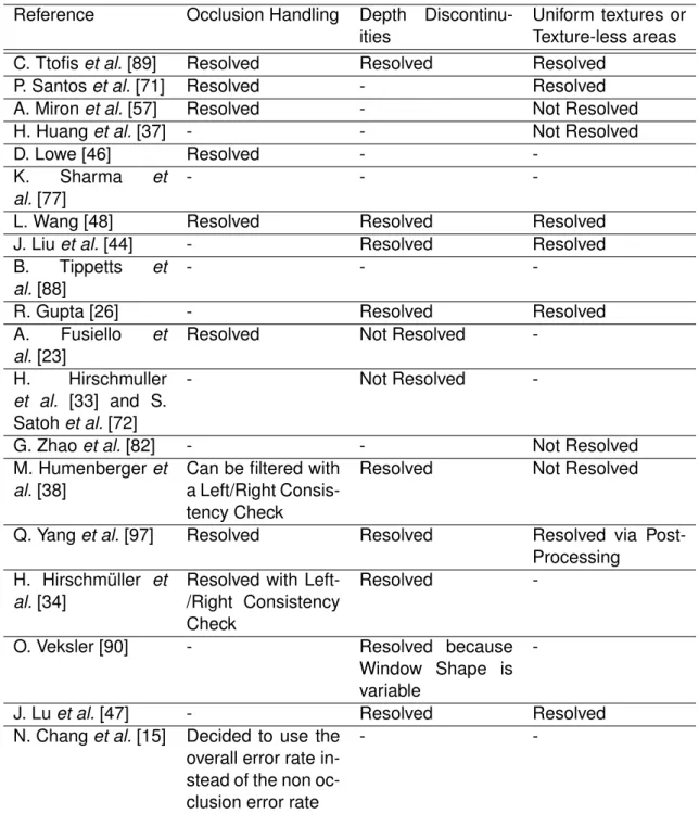
3.3 Disparity Map Calculation Methods Review . . . 40

3.4 Conclusion . . . 49

CONTENTS 3

4.1 Introduction . . . 51

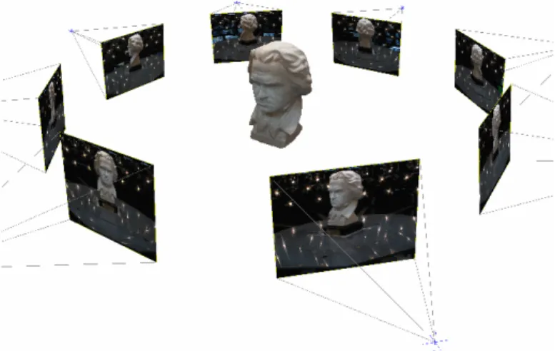
4.2 Multiple View 3D Scene Reconstruction . . . 51

4.3 Related Work . . . 53

4.4 Conclusion . . . 55

II Disparity Map Computation in WMSN 57 5 Using Disparity map techniques in WMSN 59 5.1 Introduction . . . 59

5.2 Stereo Vision methods applicable on WMSNs . . . 60

5.3 Experimentations Related to Complexity . . . 61

5.4 Wireless Multimedia Sensor Network deployment for disparity map calcu-lation . . . 66

5.5 Experimentations Related to Coverage . . . 71

5.6 Conclusion . . . 75

III 3D Reconstruction Model using Disparity Map in WMSN 77 6 Disparity Based Reconstruction Model 79 6.1 Introduction . . . 79

6.2 Problematic . . . 79

6.3 Proposed Framework . . . 81

6.3.1 Disparity computation based on binary tree distribution . . . 81

6.3.2 Discarding Similar Disparity . . . 84

6.3.2.1 Monitoring algorithm . . . 84

6.3.3 Disparity classification using Principal Component Analysis . . . 84

6.4 Disparity based reconstruction . . . 90

6.4.1 Triangulation . . . 90

6.5 Experimentation Results . . . 94

6.5.1 Nodes Distribution Scenarios . . . 94

6.5.2 Tree topology . . . 95

6.5.3 Another sensor deployment topology . . . 99

6.5.4 Indoor scene . . . 103

4 CONTENTS

IV Conclusion 107

7 Conclusion 109

7.1 Thesis Summary, Back to the Main Contributions . . . 109 7.2 Future Works and Perspectives . . . 111

L

IST OF

F

IGURES

1.1 Limitations of WMSNs . . . 12

1.2 Phases of our system . . . 13

1.3 Complete pipeline of the contributions with reference to the thesis chapters. 17 2.1 General WMSN layout . . . 21

2.2 WMSN architectures . . . 24

3.1 Disparity map computation process . . . 29

4.1 Multiple View 3D Scene Reconstruction example . . . 52

4.2 Triangulation . . . 52

4.3 CopyMe3D: Scanning and Printing Persons in 3D [81] . . . 54

5.1 Phases of our system . . . 60

5.2 Different views of the scene . . . 62

5.3 Disparity Map using SAD and SSD . . . 63

5.4 Processing time per resolution, views and number of pairs. . . 64

5.5 Proposed model . . . 66

5.6 Occlusion and overlapping problems in video sensor network coverage . . 67

5.7 Stereo vision system baseline and orientation . . . 69

5.8 Stereo Coefficient principle . . . 70

5.9 Indoor scene: elderly man walking in his private bedroom . . . 71

5.10 Outdoor scene: random populations walking in city streets . . . 72

5.11 Camera positions from top . . . 72

5.12 Applying SSIM on a computed disparity map of two different views . . . 73

6.1 General framework for 3D reconstruction based on DM . . . 86

6.2 Binary tree applied on the system . . . 87

6.3 Algorithm flowchart . . . 88

6.4 Monitoring Principle . . . 89

6.5 Triangulation . . . 91

6 LIST OF FIGURES

6.7 Reconstructed scene from left and right images . . . 93

6.8 Our tree topology . . . 94

6.9 Tree topology for house monitoring . . . 96

6.10 Real house scene image set from outdoor . . . 97

6.11 House disparity maps . . . 98

6.12 Tree scenario PCA results . . . 98

6.13 House 3D reconstruction results . . . 99

6.14 Real car scene . . . 100

6.15 Car disparity maps . . . 101

6.16 Ring PCA results . . . 101

6.17 Indoor scene . . . 103

6.18 Indoor scene disparity maps . . . 104

ABBREVIATIONS

WSN . . . Wireless Sensor Network

WMSN . . . Wireless Multimedia Sensor Network

CMOS . . . . Complementary Metal Oxide Semiconductor HVS . . . Human Visual System

QoS . . . Quality Of Service

SAD . . . Sum of Absolute Differences SSD . . . Sum of Squared Differences PSNR . . . . Peak signal-to-noise ratio SSIM . . . Structural Similarity Index MSE . . . Mean Squared Error

PCA . . . Principal component analysis AD . . . Absolute Differences

GPU . . . Graphical Processing Unit SD . . . Squared Differences

SIFT . . . Scale Invariant Feature Transform SMW . . . Symmetric Multi Window

MRF . . . Markov Random Fields NCC . . . Normalized Cross Correlation DSP . . . Digital Signal Processor RT . . . Rank Transform

CT . . . Census Transform FW . . . Fixed-size Window MW . . . Multiple Windows AW . . . Adaptive Windows

ASW . . . Adaptive Support Weights WTA . . . Winner Takes All

8 abbreviations

BP . . . Belief Propagation SGM . . . Semi-Global Matching IoT . . . Internet of Things SFM . . . Structure From Motion SFS . . . Shape From Silhouette TOF . . . Time of Flight

FOV . . . Field of View SSIM . . . Structural Similarity

A

CKNOWLEDGMENTS

This thesis is dedicated to my parents, specially my father Atty. Charbel TANNOURY, my mother Maguy and sisters Carmen and Josianne who they didn’t stop supporting me during all my life stages.

A special thanks to my role model, my uncle Abbot Paul TANNOURY, who helped and advised me in all my life’s phases.

I would like to thank my supervisors, Prof. GUYEUX, Dr. MAKHOUL and Dr. DARAZI for their guidance and support.

I would like also to thank Reverend Rector Germanos GERMANOS, Reverend Rector Michel JALEKH, Reverend Fathers Raymond HACHEM, Joe BOU JAOUDE, Toufik MAATOUK, and Mr. Tony Reaidy from the Antonine University for their continuous motivation to pursue my PhD.

Very special thanks to my colleagues in the world of research, who I met in different conferences and events. Without missing the authors who I cited, without them we cannot achieve the required improvements.

I want to thank my friends, my colleagues at Antonine University who I enjoy working and collaborating with in different projects and challenges.

1

I

NTRODUCTION

1.1/

G

I

Environmental monitoring and surveillance are gaining more attention these days. Hence, remote monitoring for quality control and event prevention is a requirement. Wireless Sen-sor Networks (WSN) was introduced as a solution for environmental surveillance [76], providing continuous observation of a place or an ongoing activity in order to gather in-formation of a particular physical phenomenon. Basically, collected data associated with WSN are related to acoustics, light, humidity, temperature, imaging, and seismic, etc. A Wireless Multimedia Sensor Network (WMSN) is a subset of WSN, it is composed of interconnected nodes, mostly cheap CMOS (Complementary Metal Oxide Semiconduc-tor) cameras, interacting with each other and capturing multimedia data (audio/video) describing their environment. During the last few years, many researchers focused on WMSNs because of their easy implementation related to their small size, their hard-ware low cost and their diversity of applications. Many challenges arise in WMSNs like high bandwidth demand, low energy consumption, efficient processing algorithms, and application-specific Quality of Service (QoS).

However, nowadays many activities in real time monitoring require more insight on an ongoing activity in order to gather information related to the depth of an object or if a building is subject to a progressive deformation. This particular information is related to the 3D representation of an object or the environment and cannot be delivered with tra-ditional collected data. Most of existing 3D reconstruction techniques [69] use advanced and expensive cameras, centralized server schema, and network topology to reconstruct all scene objects in an acceptable period of time. Most of these techniques are not in real-time.

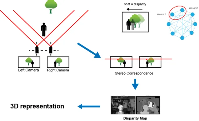
Stereo Vision is used to represent a detailed environment via multiple algorithmic meth-ods to define the surrounding world we see, based on multiple images taken from different angles. A Stereo Vision system is composed by two stereo cameras (left camera and right camera) that capture simultaneously two images from the same scene. The pair of im-ages is processed to calculate a disparity map that recovers the Depth information. The disparity map is a gray-scale image resulted from a Stereo Correspondence algorithm in order to represent corresponding pixels that are horizontally shifted between the left image and the right one. There are many methods and algorithms to solve this problem that differ in accuracy and time consumption.

Our contribution is to introduce the use of the disparity map that is computed via two or several images in order to monitor the depth information in an object or another

12 CHAPTER 1. INTRODUCTION

nomenon under surveillance using WMSN.

Sensor nodes are driven by batteries and have very low energy resources, so the pri-mary limiting constraint for WMSNs is the energy consumption that affects the network lifetime. The radio consumes the majority of the system energy in WMSNs (listening & transmitting). So an efficient WMSN should minimize communication between nodes. In our context, we oversee to use WMSN to make a 3D-depth representation of an object or an intrusion in a scene. Our main challenge is to gather 3D-depth representation while maintaining low power consumption, high speed, and QoS in WMSNs.

Another added values of our proposed method is the processing of data locally based on various nodes, hence calculating the disparity map between various images of the same scene and then transmitting it to the coordinator via the network. Consequently, the transmission of high resolution images is reduced between sensor nodes. For a pair of video sensors, only low resolution gray-scale disparity maps are transmitted on the network in addition to a reference image. Our aim is to have a dynamic, scalable, and efficient network for real time monitoring purposes. Because real-time 3D scene reconstruction utilizing centralized procedures is impossible for very large systems, but the use of distributed computation can scatter the computation over the different sensors in the network, and so decrease the computation cost on a single node.

1.2. OBJECTIVES AND PROBLEM STATEMENT 13

Figure 1.2: Phases of our system

Accordingly, two major constraints are addressed. First, high power consumption caused by high transmission rate. Second, sensing/processing capabilities for event detection and 3D reconstruction.

1.2/

O

WMSNs consist of devices (called nodes) for acquisition and transmission, deployed in an area of interest. These networks are applied particularly to prevent or detect natural dis-asters, monitor fires, retrieve vital signs from a patient, or even track military troops and make nuclear attacks assessments, etc. Subject to energetic and computational con-straints, sensor networks have limited processing and communication capabilities, but different domains profit from their miniaturization of hardware. The context of application that we envisage is the 3D information(s) acquisition and the supervision by a network of multimedia sensors. We thought about the surveillance of borders, private property, the management of public events, etc. These networks must detect thefts, traffic violations, unlawful territory, car accidents, and even unexplored places. Thus produce audiovisual data relevant for real-time or retrospective use (in subsequent surveys). We will consider as known the parameters describing the sensors, carrying directional cameras and defin-ing the captured area limited to a portion of a cone: the range of detection, field of view and orientation. On the other hand, the access to several sources of image/video data provided by cameras often allows a more accurate interpretation of events: views taken from different points can help to solve the occlusion problem. Moreover, even without occlusion, a view obtained from a single source may be insufficient to make a decision, while the combination of many sources would lead to a safer interpretation. Finally, as the camera image is a planar projection, correlating several perspectives of the element can help a better identification. Stereoscopic vision is associated with the fact that the Human Visual System (HVS) perceives a scene in 3D by simultaneously viewing a scene from slightly different positions. Therefore, providing pairs of stereo images simultaneously for each eye, makes the scene perceived in 3D by the human brain. The disparity map rep-resents the difference between horizontal disparity term between the left image and the right one. Taking into account the nature of the multimedia content, we intend to exploit

14 CHAPTER 1. INTRODUCTION

the disparity map between the different views to acquire the scenes in 3D via WMSNs. The objectives of the thesis are summarized by:

• Maximize the lifetime of the sensors, this responding to a common problem of WSNs. Hence the need to aggregate the captured data. One of the objectives would be to be limited to a reference image of the scene and to exploit the disparity map instead of sending all the images of the different sensor nodes.

• Guarantee the largest coverage (Quality of Service).

Thus we proposed to dynamically adapt the parameters of the reconstruction of the scene on sensing and aggregating level. Different aggregation solutions have been developed in the context of traditional scalar sensor networks [11, 61], but they are not adapted to WMSNs because of the nature and volume of the data exchanged.

1.3/

M

The primary objective of this work is to design an efficient 3D scene reconstruction mon-itoring system. The traditional WMSNs capture images and videos and send them via aggregator(s) to a final gateway where the server(s) interprets the multimedia data in order to take a decision or trigger an alert.

• Multimedia data are rich and have large size so they affect directly the power con-sumption of the overall network. On the other hand, disparity maps are low size gray-scale images, holding the depth value which is sufficient to detect a change or intrusion in the scene on the nodes level before reaching the server. So we pro-posed to calculate disparity maps on the nodes level and transfer them to the server. In this way, we decrease the size of the transmitted data, while holding an impor-tant parameter, sufficient for event detection (ex.: change in the depth of a water container) on the node(s) level or 3D scene reconstruction on the server level. • To calculate these disparity maps, we have a big range of existing methods, divided

into global and local methods. So we started by studying all WMSNs applications, constraints, and limitations. Then we surveyed disparity map calculation methods and algorithms, resulting a table of acceptable solutions to use in the context of WM-SNs. We focused on the processing clock-rate since sensors have low processing power, compared to video graphic cards or computer CPUs. We payed attention for the image resolutions, because camera sensors have low resolution(s). And then, hardware requirements are also a constraint, methods that can be implemented on FPGAs are acceptable for our context.

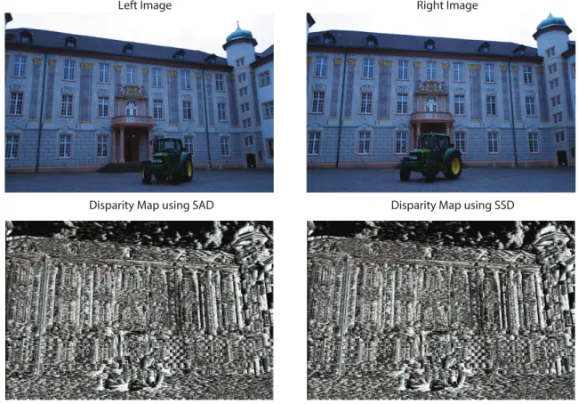
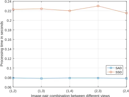
• Then we experimented two local methods: SAD and SSD. The first experimentation was made on existing captured online dataset. We found that the processing time increases linearly with the images resolutions and the number of pairs. SAD over-performed SSD in terms of processing time and complexity.

1.4. THESIS OUTLINE 15

• We have chosen SAD as convenient method to calculate disparity maps between the couples of nodes. We have created a virtual simulation of a real indoor and outdoor environment. Then we have deployed virtual nodes with different angles and distances to explore the use of disparity maps, and define the best sensors deployment and reach the required monitoring coverage.

• We have used Structural SIMilarity (SSIM) as a criterion to calculate the quality of the disparity maps. Existing researches used a ground truth disparity map as a best quality reference, and compared their calculated disparity maps to it. In our context, we don’t have a ground-truth so our approach was to calculate SSIM between a captured image and a calculated disparity map monitoring the same region. So a high SSIM reveals a high respect of the structure, so it is a good disparity map that can be transferred to the server.

• Our simulations showed that SSIM increases with the distance between the left and right camera sensor (baseline). Wide baselines are recommended for indoor scenes to ensure a small depth error. For outdoor scenes, it is better to monitor long ranged targets and increase the angle between the sensors.

• After using and exploring SAD and the deployment criteria for our sensors, we started defining the network model for our 3D scene reconstruction WMSNs based system. Mean Squared Error (MSE) calculates the similarity between the dispari-ties and helped us to remove unnecessary maps, thus decreasing the transmission rate on the network.

• We have designed different models and scenarios and focused on tree-based net-work model, which is very efficient to monitor a high range of field of views and also decreases the transmission rate.

• Principal Component Analysis (PCA) is used to cluster the received disparity maps from the nodes to the server. PCA regrouped the disparity maps, in this way, the server will make a 3D scene reconstruction using a couple of disparity maps, but not all of them. This depends on the required region to monitor. For example, a scene with 3 objects, a car, tree and house. In case we need to reconstruct the car, PCA regroups the car disparity maps, then the server will reconstruct it.

• Finally, we applied a 3D scene reconstruction algorithm on the calculated disparity maps and extracted the 3D information for the monitored scene. The 3D information is clear and it is an added value compared to existing systems, that only uses flat colored images.

1.4/

T

O

The overall organization of the thesis is presented in Figure 1.3.

• The first part, which is divided in two chapters.Chapter 2 studies the state of the art in the domain of WMSNs. Their applications, network technologies, structure, dif-ferent architectures, and challenges. WMSNs have difdif-ferent limitations like energy

16 CHAPTER 1. INTRODUCTION

consumption, high bandwidth demand, architectures and protocols flexibility, scala-bility, localized processing and data fusion, reliascala-bility, and Quality of Service (QoS). Chapter 3 deals with understanding different stereo vision algorithms, mainly global and local methods. This helped us to regroup disparity map calculation methods ap-plicable in the context of WMSNs. We surveyed them and chosen a couple of stereo vision algorithms, specifically the so-called Sum of Absolute Differences (SAD) and Sum of Squared Differences (SSD).

• The second part of this manuscript is devoted to our personal contributions by apply-ing disparity map calculation methods in WMSNs for different surveillance scenar-ios. We experimented SAD and SSD on simulated virtual scenes in order to chose the best stereo vision algorithm for efficient WMSNs monitoring system, based on 3D scene reconstruction. Existing research in stereo vision field uses advanced and expensive technologies. We compared our computed disparity maps to exist-ing ground-truth maps calculated usexist-ing laser scanners or depth sensors. We used Structural Similarity Index (SSIM) and Peak Signal-to-Noise Ratio (PSNR) as qual-itative measurements for low cost disparity map quality. So we defined the optimal sensor nodes deployment with different ranges, field of views, nodes number, and view angles. This ensure an acceptable high quality disparity map for low cost WM-SNs implementation.

• The third part defines the reconstruction model of the network in the first chapter, and shows real experimentation driven by real low cost camera sensors in the last one. This will generalize a global system model, based on dynamic parameters like angle, distance, similarity, and variance, ready to use for 3D scene reconstruction using WMSNs.

1.4. THESIS OUTLINE 17 Figure 1.3: Complete pipeline of the contr ib utions with ref erence to the thesis ch apters .

18 CHAPTER 1. INTRODUCTION

1.5/

P

[1] A. Tannoury, R. Darazi, A. Makhoul, and C. Guyeux. Introducing disparity map for 3d scene reconstruction in wireless multimedia sensor networks. Ad Hoc & Sensor Wireless Networks journal, May 2017. Technical report and submitted article [2] A. Tannoury, R. Darazi, A. Makhoul, and C. Guyeux. Introducing disparity map

for monitoring and surveillance in wireless video sensor networks. In International Conference on Computational Science (ICCS 2016), 2016

[3] A. Tannoury, R. Darazi, C. Guyeux, and A. Makhoul. Efficient and accurate monitor-ing of the depth information in a wireless multimedia sensor network based surveil-lance. In 2017 Sensors Networks Smart and Emerging Technologies (SENSET), pages 1–4, Sept 2017

[4] A. Tannoury, R. Darazi, A. Makhoul, and C. Guyeux. Wireless multimedia sensor network deployment for disparity map calculation. In 2018 IEEE Middle East and North Africa Communications Conference (MENACOMM), pages 1–6, April 2018 [5] A. Tannoury, R. Darazi, A. Makhoul, and C. Guyeux. Distributed disparity based

method for 3d scen reconstruction in wireless multimedia sensor networks. Multi-media Tools and Applications, September 2018. submitted journal

I

WMSN, D

ISPARITY

M

AP AND

3D S

CENE

R

ECONSTRUCTION

2

U

NDERSTANDING

WMSN

2.1/

I

Wireless Sensor Networks (WSNs), composed of scalar sensors, shifted to Wireless Mul-timedia Sensor Networks (WMSNs) capable to capture scalar data, images, audio, and video. The development of inexpensive CMOS cameras and distributed signal processing and coding technologies gives the WMSNs the capability to deliver multimedia content. WMSNs nodes are battery-powered with sensing, processing, and wireless communicat-ing capabilities [3]. The network is composed of large number of sensor nodes deployed in a scene of interest with one or many base stations as shown inFigure 2.1. The base station (sink) is the main network controller or coordinator. All gathered information from different sensor nodes are collected, stored, and processed by the sink. The sink plays also the role of a gateway to other networks. Note that sinks are mostly located in a close distance to the nodes, as long range radio communications consume high energy. Let us now investigate various technical aspects of such networks, by focusing first on their applications.

Figure 2.1: General WMSN layout

2.2/

WMSN

A

WMSN are used in many applications covering various fields like real-time objects track-ing in industrial production, scene monitortrack-ing in agriculture, and vital signs monitortrack-ing in health-care, etc. Examples of such applications are listed hereafter.

22 CHAPTER 2. UNDERSTANDING WMSN

• WMSNs for surveillance: Which develop old surveillance systems by using a large deployment of low-cost and low-powered audiovisual nodes. It helps to monitor, detect, and record activities like thefts, bridges structure changes, automobile acci-dents, traffic violations, or any cautious behavior [10]. Adding to this list, the audio data can be used to sense unusual sounds such as shooting, explosions, etc. • WMSNs for traffic avoidance, enforcement, and control systems: Numerous

countries suffer from traffic, specially on the highway. So using WMSNs, drivers can view all road status and decide where to go or park their vehicles. To reach this goal, GPS data can also be added to multimedia data.

• WMSNs for advanced healthcare: WMSNs can provide universal healthcare ser-vices by monitoring patient parameters like pulse, blood pressure, and so on [58]. Data can be recorded and transmitted to the monitors on real-time. Multimedia data is much richer than scalar one for diagnostics and physiological data.

• WMSNs for environmental and house monitoring: WMSNs are very convenient for habitat and house monitoring because of their full coverage possibility of imple-mentation. For example, they can monitor animals in a zoo or island in order to study the percentage of leaving creatures [9]. At home, thefts or any intrusions can be detected easily with all details. The system can communicate with an emergency service for intervention in case of flood, fire, or chemical detection for example. • WMSNs for industrial or infrastructure control: Deploying a network of video

sensors in a scene can give us the opportunity to monitor visible and non-visible objects from different views, for quality control or plant monitoring [8]. Researchers visually monitored construction and operation of buildings, bridges, or any type of civil infrastructure. Note that augmented reality can cooperate with WMSNs to de-velop amazing efficient practical applications like visualizing 3D representations of environmental information in real time using smart phones [25].

• WMSNs for military applications: A bunch of military applications, like in [41], use WMSNs for monitoring friendly forces equipment and ammunition, battlefield surveillance, investigation of opposing forces and terrain, targeting, and nuclear, biological, and chemical (NBC) attack detection and reconnaissance, and finally battle damage assessment.

2.3/

WMSN C

WMSNs consist of four main components: Wireless Multimedia Node (WMN), Wireless Cluster Head (WCH), Wireless Network Node (WNN), and Base Station (BS). WMN and WCH focus on data processing, and WNN on wireless network communications.

• Wireless multimedia node [4]. Each node is composed of a camera or audio sen-sor, a processing unit, a communication unit, and finally a power unit. The camera sensor has a Field Of View (FOV) of the scene. Visual processing is achieved by the processing unit. Note that WMSNs can be implemented in a way where events

2.4. WMSN NETWORK ARCHITECTURE 23

are detected before transmitting images (frames) through the network. If no useful event is detected, images are discarded.

• Wireless cluster head. Several WMNs send data to the cluster head. Each WCH is composed by a processing unit, a communication unit, and a power unit. Some-times WMNs FOV overlaps, so the WCH will perform an exaggeration to remove overlapping frames.

• Wireless network node. The WNN is similar to traditional wireless sensor network and lies as a communication unit and a power one. The communication unit sends the data between nodes as long as it arrives at the base station.

• Base Station, which gathers all the data and has powerful processing and energy capabilities. It is a kind of server.

2.4/

WMSN

Most of scalar WSNs have a flat architecture of distributed homogeneous nodes. These networks measure physical phenomenon like temperature and provide as an output a scalar value for each measurement. WMSNs have been introduced in emerging appli-cation fields that raise the need to have alternative network architectures. Scalability, efficiency, and QoS are the main requirements for new network architectures. Gener-ally speaking, WSNs architecture can be either single-tier flat, single-tier or single-tier clustered, or multi-tier one, as shown inFigure 2.2.

24 CHAPTER 2. UNDERSTANDING WMSN

(a) Single-Tier Flat Architecture

Internet

Sink

Gateway Storage Hub

WMSN

(b) Single-Tier Clustered Architecture

Internet Sink Gateway Storage Hub CH CH (c) Multi-Tier Architecture Internet Sink Gateway Storage Hub Video sensors Image sensors Scalar sensors Figure 2.2: WMSN architectures

2.5. WMSN CHALLENGES 25

• Single-tier flat architecture: The network is set up with homogeneous sensor nodes with the same capabilities and functionality. All the nodes perform functions like image capturing, multimedia processing, or data delivery to the sink. This flat architecture is easy to manage and the multimedia processing is distributed among the nodes, contributing to the extension of the network life time.

• Single-tier clustered architecture: The network is deployed with heterogeneous sensors like video, audio, and scalar ones. All different sensors within each cluster relay data to a Cluster Head (CH), which is connected with the sink directly or through other CHs.

• Multi-tier architecture: This network is deployed using heterogeneous sensors in a multi-tier architecture.

– The first tier performs simple tasks via scalar sensors like motion detection. – The second tier performs more complex tasks like object detection or

recogni-tion.

– The third tier may achieve an object tracking via powerful high resolution cam-era sensors, which is a complex task to do.

Each tier can have a central hub to enhance data processing and communication with the higher tier. This architecture meets different needs while balancing between costs, coverage functionality, and reliability requirements.

2.5/

WMSN

In this section, we discuss important limitations and challenges for WMSN applications such as energy consumption, high bandwidth demand, architectures and protocols flex-ibility. And their scalability to support heterogeneous applications, localized processing, data fusion, and finally reliability and QoS.

2.5.1/ ENERGY CONSUMPTION

The essential limiting factor in WMSN is energy consumption, because sensor nodes are driven by small batteries and have very low energy resources. So energy optimization is a dominant consideration no matter what is the application or objective. Transmission consumes the majority of the energy. So it is very important to decrease transmission distances between nodes and the amount of transmitted data. Moreover, energy con-sumption increases by node electronics for sensing and processing [39]. As an illustra-tion, Zhao et al. estimated in [103] that 64kB of data consumed 377µJ of power for radio (data transmission) and 0.00195µJ for program execution (data processing).

26 CHAPTER 2. UNDERSTANDING WMSN

2.5.2/ HIGH BANDWIDTH DEMAND

WMSNs differ from the traditional WSNs in delivering multimedia content such as images, audio, and video streams. Hence, it requires a significant bandwidth. For example, the maximum transmission rate of IEEE 802.15.4 components such as Crossbow’s TelosB or MICAz motes is 250 kbps [63]. With the same power consumption, WMSNs require higher data rates when it comes to high quality images and video with high pixel resolution and high number of frames per second.

2.5.3/ ARCHITECTURE SCALABILITY AND PROTOCOL FLEXIBILITY

The WMSNs design should respect scalability and flexibility to give the opportunity to extend the network in the future. Multimedia processing algorithms and protocols, for their part, should be flexible to support a wide diversity of applications while respecting the energy, QoS, delay, and security (privacy) limitations of WMSNs. Note that mobility can avoid the effect of environmental risks like rain, snow, high humidity, etc.

2.5.4/ LOCALIZED PROCESSING AND DATA FUSION

Transmitting multimedia content requires huge bandwidth and hence transmitting uncessed content will need a high cost. An advantage is to benefit from multimedia pro-cessing and data fusion algorithms in order to reduce the high bandwidth requirement and also decrease the transmission cost.

2.5.5/ RELIABILITY

Another great challenge in WMSNs is the reliability of the node and data transfer. The power decrease is the main cause to drop down the node. Harsh environment or physical damage can also affect the node. Sensor nodes may work in high traffic environment, indoor, outdoor, underwater, little house, or huge building. Also, big packet retransmission causes power decrease. So the reliability of the WMSNs design to resist against such undesirable accidents is a must, and can be done by creating robust physical structure for the nodes and reliable power efficient transport functions.

2.5.6/ QUALITY OFSERVICE

The requirements of WMSNs are different from traditional WSNs using scalar sensors. Multimedia data covers images, audio, and video streams. Camera nodes can capture

2.6. PROBLEMATIC AND SOLUTION 27

images in a short time but video streams take more time and require continuous captur-ing and delivery. This differs from an application to another, where in some surveillance applications the real time capability is mandatory. Consequently, efficient hardware and software techniques are required to maintain the recommended QoS by a specific appli-cation.

2.5.7/ WMSNS CHALLENGES FOR DISPARITY MAP COMPUTATION AND STEREO

RECONSTRUCTION

The already mentioned limitations emphasize the challenge to increase the network life-time by decreasing the power consumption. The latter is one of the main problems in designing future in-network processing techniques. To achieve a low cost transmission, we use gray scale disparity map instead of colored images. Spatial correlation between different sensor nodes also plays an essential role: for each pair of sensors, only a differ-ence in the frames will trigger the recapturing of two images, therefore leading to recom-pute the disparity map.

Otherwise, only one node will be active and the second one will enter the sleep mode. In this case, no need to send, on real time, new images to the sink. Only one image with the disparity map we calculated before are sufficient to monitor the scene. High band-width demand is resolved by transmitting black and white disparity maps without colored images. The fact of activating one node from the pair and sleeping the other one will de-crease processing and transmission on distributed pairs level. In the next chapter (resp. Chapter 3), we will survey all disparity map calculation methods and choose the group of methods that can be handled by WMSN nodes in terms of computational demands.

2.6/

P

S

The main problematic can be summarized as follows: how to create an efficient monitor-ing based on WMSNs that lasts for a long period of time, works in real-time and with a good QoS?

The transmitted data may be used later for 3D scene reconstruction or event detection. The centralized network topology is unpractical for 3D real-time applications, so we will use a distributed wireless multimedia sensor network. By this way, the calculation and processing is divided on all sensor nodes to avoid high network load and decrease energy consumption. Each couple of sensors will make a stereo matching between a pair of images in order to calculate a disparity map. Disparity maps have low size and are good enough to 3D scene reconstruction or event (difference in depth) detection, as they contain the depth values of the environment. Sending a disparity map over the network instead of sending pair of images can decrease the size of transmitted data and hence reduce the bandwidth usage.

28 CHAPTER 2. UNDERSTANDING WMSN

2.7/

C

Using WMSNs for different applications and scenarios, specially for surveillance, is gain-ful in terms of flexibility of deployment and low cost of implementation. But we should respect the pre-mentioned limitations and constraints. The scalability and mobility of these types of networks is promising to apply stereo vision on a distributed couples of sensors. But what is the complexity of a computer vision system? How it is applicable on WMSNs? What is the best disparity map calculation method or group of algorithms that performs better, and in an efficient way on sensors? The different types of network architectures open multiple questions and problematic on how these disparity maps will travel the network from node to node, or nodes to aggregator(s). The next Chapter 3 outlines all disparity map calculation methods in details.

3

D

ISPARITY

M

AP PRINCIPLES AND

COMPUTATION TECHNIQUES

3.1/

I

Disparity map represents corresponding pixels that are horizontally shifted between the left image and the right camera. New methods and techniques for solving this problem are developed each year and exhibit a trend toward improvement in accuracy and time consumption [68].

Our main focus is to choose the best solution to be applied on WMSN in an efficient way when considering energy consumption, storage capability, communication cost, and quality of service. Indeed, in real-time applications, a fast and accurate depth calculation method is a must. Various methods have been classified into local methods and global ones.

All disparity map calculation steps are discussed in the next section.

3.2/

S

The 4 main steps for stereo vision algorithm are represented inFigure 3.1.

Figure 3.1: Disparity map computation process

30 CHAPTER 3. DISPARITY MAP PRINCIPLES AND COMPUTATION TECHNIQUES

3.2.1/ MATCHING COST COMPUTATION

In this stage, given the values of two pixels, we determine if they accord to the same point in the scene or not. The matching cost is computed at each pixel for all considered pix-els. The disparity is the difference in pixel intensity between a pair of the matching pixels in two images and can be related with depth values via 3D projection [68]. Pixel-based matching costs can be done with absolute differences, sampling-insensitive absolute dif-ferences, squared difdif-ferences, or truncated versions. These algorithms can be used for gray-scale or colored images [33]. H. Ibrahim et al. introduced the fact that area based (window based) techniques can offer better data than individual pixels based ones [68]. These techniques are more accurate, because in the matching process, the entire set of pixels associated with image regions is used. The matching cost is calculated over an aggregating window that can have the form of a square or rectangle and may have a fixed or adaptive size.

Window-based technique has the following limitation: it considers that all the pixels in a support window have the same disparity values. This is not just the case near depth discontinuities or edges. Therefore, any inappropriate selection of the size or shape of the matching window can cause a low depth estimation.

3.2.1.1/ ABSOLUTEDIFFERENCES (AD)

The AD algorithm aggregates the differences in intensity (luminance) between the pixel in the left image and the corresponding pixels in the right one, as following:

AD(x, y, d)= |Il(x, y) − Ir(x − d, y)| (3.1)

• (x,y,d) represents the disparity map coordinates; • (x,y) are the coordinates of the pixel of interest; • d is the disparity (depth) value;

• Il used as left reference image;

• Irused as right target candidate image.

AD algorithm is the simplest matching cost algorithm and can be used, as in [92], for real-time stereo matching using a Graphical Processing Unit (GPU). It is functional for little textured regions but it may produce a non-smooth disparity map for a highly tex-tured image. An updated version of AD, called Truncated Absolute Difference (TAD), was developed and implemented by Min et al. [56] and Pham et al. [65]. It uses colors and gradients and improved the results on variations in illumination.

3.2. STEREO VISION DISPARITY MAP ALGORITHM STAGES 31

3.2.1.2/ SQUARED DIFFERENCES (SD)

The SD algorithm aggregates the squared differences between the pixel in the left image and the candidate in the right image as following:

S D(x, y, d)= |Il(x, y) − Ir(x − d, y)|2. (3.2)

Before improving the flattening of edges near depth discontinuities with a bilateral filter by Yang et al. in [96], the initial generated disparity maps contained noise. Miron et al. [57] compared SD algorithm with many other matching cost functions for intelligent vehicle applications and produced largest error because SD are reactive to brightness and noise, especially for real-time environment.

3.2.1.3/ FEATURE BASED TECHNIQUES

Huang and Wang divided the feature based techniques into [37]:

1. Visual features of images: Clearly detected characteristics, such as contour, shape, brightness, contrast, color, and texture.

2. Statistical characteristics of images: The statistical distribution of image pixels, such as amplitude mean, maximum, minimum, median, histogram, variance, and entropy.

3. Transformation features of images: Images using a variety of different mathe-matical transformations to the target image are mapped to transform domain, and then features are extracted. Commonly used methods include: Fourier transform, Hough transform, KL transform, Wavelet transform, and Gabor one. In the process of image recognition, statistical features and transform features are generally used to describe and identify an object.

Scale Invariant Feature Transform (SIFT) extracts typical invariable features from images, used for stereo matching (stereo vision). These features do not change with image scale or rotation, and provide strong matching across a considerable range of affine distortion, modification in 3D viewpoint, noise, and change in illumination [46]. The following defines the crucial steps for computation used for image features generation.

1. Scale-space Extrema Detection. It uses a Difference-of-Gaussian function to look for minimum and maximum interest regions that are invariant to scale and orienta-tion.

32 CHAPTER 3. DISPARITY MAP PRINCIPLES AND COMPUTATION TECHNIQUES

2. Keypoint Localization. It estimates the location and scale of each keypoint, and then eliminates the unstable keypoints.

3. Orientation Assignment. It assigns one or more orientation(s) to each keypoint location built on local image gradient directions.

4. Keypoint Descriptor. It measures the local image gradients at the selected scale in the region around each keypoint. They are transformed into a representation that allows for significant levels of local shape distortion and change in illumination.

Sharma et al. [77] developed an updated disparity map algorithm using features from the SIFT for autonomous vehicle navigation by modifying the SIFT algorithm. They reduced computation time by improving the feature matching process using a Self-Organizing Map (SOM). Compared with the original SIFT algorithm, the computational time and cost are significantly reduced but the complete disparity map cannot be acquired.

Liang Wang concluded in his thesis [48] that feature-based approaches try to calculate correspondences for distinct feature points that can be matched unambiguously. Match-ing works fine on noticeable features. But it produces sparse disparities, because it uses only the matching points derived from the targeted object features. Feature-based tech-niques present low accuracy and are insensitive to occlusion and texture less areas. Area-based approaches take into consideration larger image regions containing richer information than individual pixels, to yield more stable matches.

Liu et al. [44] combined image segmentation and edge detection for the matching cost computation in order to reduce time and cost. Because traditional global stereo matching methods used an optimized energy function to obtain accurate disparity, but it needed high computation time and more memory, which confront real time processing. They tested it on indoor and outdoor scene (such as “Avatar”) and concluded that it does not preserve boundaries (discontinuities), but it is ideal for most of the scene cases with fast time.

Note that feature based techniques are not preferred, and not very used by researchers in the domain of disparity map calculation.

3.2.1.4/ SUM OFABSOLUTEDIFFERENCES (SAD)

The SAD algorithm calculates the absolute difference between the intensity of each pixel in the reference block and that of the corresponding pixel in the target block:

S AD(x, y, d)= X

(x,y)∈w

|Il(x, y) − Ir(x − d, y)| (3.3)

3.2. STEREO VISION DISPARITY MAP ALGORITHM STAGES 33

The SAD algorithm is a popular algorithm for matching cost computation and it can work in real time with low computational complexity. For example, Tippetts et al. [88] evaluated the SAD performances on real time human poses and a resource limited system. Gupta and Cho [26] used SAD with two sizes of correlation windows by firstly determining the aggregation cost, then improving object boundaries (discontinuities) using smaller win-dow size. The proposed algorithm computes more than 10 frames/s on real time, a sharp and dense disparity map for 3D scene reconstruction. Open source evaluations and comparisons have been experimented on benchmark Middlebury stereo datasets web-site to demonstrate qualitative and quantitative performance of the proposed algorithm and many others.

The SAD algorithm is fast but it produces low quality initial disparity maps caused by noise at object boundaries and in texture less areas.

3.2.1.5/ SUM OFSQUARED DIFFERENCES (SSD)

Equation 3.4 summarizes the SSD algorithm:

S S D(x, y, d)= X

(x,y)∈w

|Il(x, y) − Ir(x − d, y)|2. (3.4)

Fusiello et al. [23] tested SSD algorithm on multiple fixed window blocks searching for the smallest error, to select an appropriate pixel of interest in the disparity map. They introduced a novel probabilistic stereo method based on Symmetric Multi Window (SMW) algorithm. In this paper, they performed matching by correlation between different types of windows in the two images, and enforcing the left-right consistency constraint. This re-quires the uniqueness constraint where each point in image 1 can match at maximum one point in image 2. This is improved by using a probabilistic SMW using Markov Random Fields (MRFs). MRFs are largely used in image restoration, segmentation, and recon-struction. In [23], authors experimented the algorithm on indoor (“Head” stereo pairs from the Multiview Image Database, University of Tsukuba) and outdoor scenes (castle, trees and parking meters).

Many authors achieved better results in terms of speed than Fusiello’s work, but by imple-menting it on a platform with a GPU. That makes it impossible for WMSN usage. There is little research papers on the use of SSD algorithm for stereo vision disparity map cal-culation.

3.2.1.6/ NORMALIZED CROSS CORRELATION (NCC)

Another method to determine the correspondence between two windows around a pixel of interest is NCC. The following Equation 3.5 is the formula for NCC:

34 CHAPTER 3. DISPARITY MAP PRINCIPLES AND COMPUTATION TECHNIQUES (3.5) NCC(x, y, d)= P (x,y)∈wIl(x, y).Ir(x − d, y) s X (x,y)∈w I2_l(x, y). X (x,y)∈w Ir2(x − d, y) .

NCC tends to blur depth discontinuities more than many other matching costs, and can only be used with local methods due to its window-based design [32]. Satoh [72] pro-posed a simple low-dimensional features approximating NCC-based image matching method, because NCC is robust to intensity offsets and changes in contrast, but it is computationally expensive. SAD or SSD are less robust against geometrical distortion (occlusion, clipping, perspective projection, illumination distortion), but simpler and suit-able for hardware implementation such as digital signal processor (DSP).

3.2.1.7/ RANKTRANSFORM(RT)

The RT matching cost is calculated by the following formula using the absolute difference between the rank from the reference image and the one from the target image:

RT(x, y, d)= X

(x,y)∈w

Rankre f(x, y) − Ranktar(x − d, y)  

 (3.6)

where Rankre f and Ranktar are calculated as follow:

Rank(x, y)= X (i, j)(x,y) L(i, j) (3.7) where L(i, j)=        0 : I(i,j) < I(x,y) 1 : otherwise (3.8) in which:

• (i,j) represents the coordinates of a neighboring pixel; • (x,y) represents the coordinates of the pixel of interest.

Equation 3.8 computes the number of neighboring pixels I(i,j) having larger values than that of the central pixel I(x,y).

Gac et al. [24] used RT for a Pipelined, Pre-fetch and Parallelized Architecture for Positon Emission Tomography (3PA – PET) and compared time performances with a PC, work-station and GPU. They obtained a reliable initial disparity map while carefully selecting the window sizes. RT deals effectively with brightness differences and image distortions but sometimes it leads to matching ambiguity when a matching pixel may look extremely similar to a neighboring one.

3.2. STEREO VISION DISPARITY MAP ALGORITHM STAGES 35

Zhao et al. [82] decreased this matching ambiguity using a Bayesian stereo matching model. So it considers not only the similarity between the couple of images pixels but also the ambiguity level of these pixels in their own image independently. They tested their algorithm on both intensity and color images with brightness differences and resulted effective corresponding 2D disparity maps and 3D scene reconstruction.

3.2.1.8/ CENSUS TRANSFORM(CT)

In CT algorithm, the results of comparisons between center pixel and its neighbor pixels within a window are translated into a bit string as follow:

Census(x, y)= Bitstring(i, j)∈w(I(i, j) ≥ I(x, y)) (3.9)

Hamming distances between the census bit strings on the corresponding match candi-dates is used to calculate the CT algorithm, as follow:

(3.10) CT(x, y, d)= X

(x,y)∈w

Hamming(Censusre f(x, y) − Censustar(x − d, y))

• Censusre f is the census bit string from the reference image;

• Censustar is the census bit string from the target one.

Humenberger et al. [38] tackled the challenge of fast stereo matching for embedded sys-tems, because these systems have the similar limitations of WMSN as memory, process-ing power, and real-time capability for robotics applications. Such limitations do not allow the use of complicated stereo matching algorithms. They handled hard areas having low texture and achieved high performance results on several, including resource-limited, systems while preserving a good quality stereo matching. They gave a detailed perfor-mance analysis of the algorithm via PC, DSP and a GPU reaching a frame rate of up to 75 FPS for 640 x 480 images and 50 disparities. They compared the algorithm with existing standards (SAD algorithm) on the Middlebury Stereo Evaluation Website and achieved a 50 % quality and top performance ranking of indoor and outdoor scenes.

CT displayed higher matching quality at object boundaries (discontinuities) than those produced by SAD algorithm. One of the disadvantages is producing incorrect matching in areas with repetitive structures. Ma et al. [49] decreased the effect of repetitive structures and proposed an updated algorithm that demonstrated greater robustness when applied to a noisy image compared with conventional CT algorithm. Errors can be reduced by combining the two algorithms SAD and CT. Because CT is sensitive to areas with repet-itive local structures and AD algorithm performs bad on large texture-less regions. So a

36 CHAPTER 3. DISPARITY MAP PRINCIPLES AND COMPUTATION TECHNIQUES

combination of SAD and CT algorithms will lead to better performance but causes an in-crease in computational complexity. Many researchers combined two methods like SAD and Arm Length Differences (ALD) or CT and gradient difference approaches to reach a better matching cost quality, but however matching ambiguities still can occur in some areas because of similar or repetitive texture patterns.

3.2.2/ COST AGGREGATION

Cost aggregation is the most crucial stage for the performance of a stereo vision disparity map algorithm, in a special way for local methods. In this stage, matching uncertainties are determined. Data obtained for one pixel upon calculating the matching cost is not sufficient for an exact matching, so cost aggregation is essentially needed. In local meth-ods, matching cost is aggregated by summing them over a support region defined by a square window centered on the current pixel of interest. Applying a simple low-pass filter in the square support window is the most genuine aggregation method. Global algorithms commonly skip the cost aggregation phase and define a global energy function including a data term and a smoothness one.

3.2.2.1/ COST AGGREGATION WITHFIXED-SIZEWINDOW(FW)

The FW method experiences an increased error rate when support window size is increased over a threshold. It requires the parameters to be set to values convenient for the particular input dataset. A rectangular support window is unsuitable for pixels near object boundaries with arbitrary shapes, and a simple discontinuity interpretation method is not strict enough to conserve edges [97]. Yan et al. [97] implemented their method on both CPU and GPU. The CPU method uses C++ and OpenCV on a Core Duo 3.16GHz CPU and 2GB 800 MHz RAM with no parallelism technique. To avoid augmenting artifacts near discontinuities, multiple methods have been developed using Shifting Window or Multiple Windows (MW), Adaptive Windows (AW), windows with Adaptive Sizes, or Adaptive Support Weights (ASW).

3.2.2.2/ COST AGGREGATION WITHMULTIPLEWINDOWS (MW)

In this method, the algorithm selects multiple windows from a number of competitors in a way where support windows produce smaller matching costs. Hirschm ¨uller et al. [34] im-plemented this technique for processing the local working environment of a tele-operated robot and revealed a main weakness for the multiple windows method: the computational cost. But it can be optimized using 5 windows and it is very effective. Veksler [90] devel-oped a fast and accurate variable window approach and mentioned that the two essentials elements to achieve accuracy are the following:

3.2. STEREO VISION DISPARITY MAP ALGORITHM STAGES 37

• Choosing a useful range of window sizes/shapes for evaluation;

• Developing a new window cost that is particularly suitable for comparing windows of different sizes.

Their method can compute window cost over any rectangular window in stable time, re-gardless of window size. It is ranked in the top 4 on the Middlebury Stereo Dataset web-site with ground truth with comparable efficiency (tested on Tsukuba, Sawtooth, Venus and Map scenes). Hirschm ¨uller et al. and Veksler revealed difficulties to preserve ded-icated pixel arrangements in disparity maps, specifically at object boundaries. This is caused by the shape of the support windows. This method is inexact for a small num-ber of candidates. The Adaptive Windows (AW) technique was developed to resolve this problem.

3.2.2.3/ COST AGGREGATION WITHADAPTIVE WINDOWS (AW)

Lu et al. [47] proposed a novel stereo correspondence algorithm producing high quality disparity estimation results even with depth discontinuities or homogeneous areas using anisotropic Local Polynomial Approximation (LPA) – Intersection of Confidence Intervals (ICI) technique. They tested and evaluated results via Middleburry Stereo Data Sets on different scenes (Tsukuba, Sawtooth, Venus, and Map) implemented on a GPU for real time applications. Chen and Su [16] expected a shape adaptive low complexity technique to eliminate computational redundancy between stereo image pairs for pixels matching. Pixels having the same depth value were grouped to reduce computations number. As the most time consuming step of stereo matching algorithm is the cost aggregation over local image regions, Fang et al. [22] published a comparative study on FW, AW, and ASW and emphasized that the best technique for cost aggregation is ASW. All the experiments were done on a NVIDIA Quadro5000 Fermi GPU.

3.2.2.4/ COST AGGREGATION WITHADAPTIVE SUPPORTWEIGHTS (ASW)

In this approach, if the intensity of a pixel is more similar to that of the anchor pixel and if it is located at a smaller distance from the anchor pixel, it will allocate a higher weight. Many researchers like Hosni et al. [35] and Nalpantidis and Gasteratos [59] used this method on a GPU and produced great results in terms of computational efficiency and quality of disparity maps.

38 CHAPTER 3. DISPARITY MAP PRINCIPLES AND COMPUTATION TECHNIQUES

3.2.3/ DISPARITY COMPUTATION AND OPTIMIZATION

3.2.3.1/ DISPARITY COMPUTATION AND OPTIMIZATION IN THE LOCAL APPROACH

The local approach uses a local Winner Takes All (WTA) strategy while selecting the disparity for each pixel in order to compute final disparities. It is defined as follow:

dp= argd∈Dmin C

0

(p, d) (3.11)

• At each pixel, it chooses the disparity associated with the minimum aggregated cost dp.

• C0(p, d) is the aggregated cost retrieved after the matching cost calculation. • D shows the set of all allowed distinct disparities.

Referencing implementations made by Cigla and Alatan [17], Zhang et al. [101], and Lee et al. [42], the disparity maps obtained at this stage contained errors like unmatched pixels or occluded regions. Because in local methods the aggregation is done through summation or averaging over support regions. So their accuracy is sensitive to noise and unclear regions. Utilizing local information from a small number of pixels surrounding the pixel of interest to make the every decision will cause this problem. This can be reduced using multiple filtering techniques in the disparity map refinement step discussed later in this article.

3.2.3.2/ DISPARITY COMPUTATION AND OPTIMIZATION IN THE GLOBAL APPROACH

The global approach makes certain assumptions about the depth of field of the scene, expressed in an energy minimization framework. In global method, the big effort is done during disparity computation step. The well-known assumption is that the scene is smooth except object boundaries and thus neighboring pixels should have very similar disparities, this is what we call the smoothness constraint in the stereo vision literature. The main target is to find an optimal energy disparity assignment function d= d(x, y) that minimizes:

E(d)= Edata(d)+ βEsmooth(d), (3.12)

where:

• Edata(d) expresses the matching costs at coordinates (x, y);

• Esmooth(d) (smoothness energy) reassures neighboring pixels to have similar

3.2. STEREO VISION DISPARITY MAP ALGORITHM STAGES 39

• β is a weighting factor.

Belief Propagation (BP) is a well-known global method that requires big computational re-sources and memory for storing image data and executing the algorithm. Another global approach is Graph Cut (GC) implemented by Wang et al. [67] to optimize the energy func-tion. Dynamic Programming (DP) assumes an ordering constraint between neighboring pixels of the same row. Arranz et al. [7] preserved high resolution disparity maps while obtaining real-time performance and keeping accurate results in the Middleburry test data set, without the requirement of parallel computing. But it fails to perform at a real time frame rate of 30 FPS for images with high resolution and different levels of disparity.

3.2.4/ DISPARITY MAP REFINEMENT

At this stage, noise is reduced and disparity maps are improved. It consists of regulariza-tion and occlusion filling (interpolaregulariza-tion). During regularizaregulariza-tion, the overall noise is reduced by filtering inconsistent pixels and little variations among pixels on disparity map. During occlusion filling, the disparity values in areas with unclear disparities are approximated. In general, it fills occluded regions with disparities similar to those of the background or texture-less areas. Left-right consistency check is used to detect occlusions.

Yang et al. [95] proposed a good algorithm that outperformed other ones on the Middle-burry data sets. Their algorithm, experimented on indoor and outdoor scenes, performs well when applied on planar surfaces, because the depth information of unstable areas is increased from the stable pixels around the neighborhood by fitting a 3D plane. The performance of Yang et al. algorithm may drop if the scene is primarily composed of smooth curved surfaces like quadratic. Heo et al. [31] proposed another algorithm for depth map and consistency check. Stereo matching and performing color consistency between stereo images are a chicken-and-egg problem, since it is not a trivial task to simultaneously achieve both goals [31]. Experimental results, on indoor and outdoor scenes, show that their method achieves both accurate depth maps and color-consistent stereo images even for stereo images with severe radiometric differences.

The main local disparity refinement techniques are Gaussian convolution, median filter, and anisotropic diffusion.

3.2.4.1/ DISPARITY MAP REFINEMENT USING GAUSSIAN CONVOLUTION

A Gaussian distribution defines weights for neighboring pixels in order to estimate dispar-ities. It reduces noise but also decreases the amount of fine details in the final disparity map. Vijayanagar et al. [91] developed a real time refinement algorithm for depth maps generated from low-cost commercial depth sensors like the Microsoft Kinect, by using the weights defined by a Gaussian Filter.