HAL Id: tel-01810835
https://tel.archives-ouvertes.fr/tel-01810835
Submitted on 8 Jun 2018HAL is a multi-disciplinary open access archive for the deposit and dissemination of sci-entific research documents, whether they are pub-lished or not. The documents may come from teaching and research institutions in France or abroad, or from public or private research centers.
L’archive ouverte pluridisciplinaire HAL, est destinée au dépôt et à la diffusion de documents scientifiques de niveau recherche, publiés ou non, émanant des établissements d’enseignement et de recherche français ou étrangers, des laboratoires publics ou privés.
Experimental and numerical study of model gravity
currents in coastal environment : bottom gravity
currents
Dhafar Ibrahim Ahmed
To cite this version:
Dhafar Ibrahim Ahmed. Experimental and numerical study of model gravity currents in coastal environment : bottom gravity currents. Other. Université de Bretagne occidentale - Brest, 2017. English. �NNT : 2017BRES0060�. �tel-01810835�
Etude Expérimentale et
Numérique de Courants
Gravitaires Modèles en
Environnement Côtier:
Courant gravitaire dense
Thèse soutenue le (01/09/2017)
Devant le jury composé de :
Mr Lalaonirina RAKATOMANANA
Professeur, Université de Rennes 1, président
Mr Innocent MUTABAZI
Professeur, Université du Havre, rapporteur
Mr Ahmed OULD EL MOCTAR
Maître de Conférences HDR, Université de Nantes, rapporteur
Mme Cécile LEMAITRE
Maître de Conférences HDR, Université de Lorraine, examinateur
Mr Didier BERNARD
Maître de Conférences HDR, Université des Antilles, examinateur
Mr Bernard POTTIER,
Professeur, UBO, examinateur
Mr Noureddine LATRACHE
Maître de Conférences, UBO, Co-encadrant de thèse
Mr Blaise NSOM
Professeur UBO, Directeur de thèse
Mr Fulgence RAZAFIMAHERY
Maître de Conférences, Université de Rennes 1, invité Présentée par
Dhafar Ibrahim AHMED
Préparée au sein de la FRE CNRS 3744 IRDLInstitut de Recherche Dupuy de Lôme
THÈSE / UNIVERSITÉ DE BRETAGNE OCCIDENTALE sous le sceau de l’Université Bretagne Loire
pour obtenir le titre de
DOCTEUR DE L’UNIVERSITÉ DE BRETAGNE OCCIDENTALE
Mention : Sciences pour l'Ingénieur Discipline : Génie côtier
Spécialité : L'Environnement ; les modèles de qualité de l'eau École Doctorale des Sciences de la Mer
University of
Western Brittany
Doctoral School of Marine Sciences
DISSERTATION
Experimental and Numerical Study of Model Gravity Currents in Coastal
Environment: Bottom Gravity Currents
Submitted by
Dhafar Ibrahim Ahmed
In partial fulfillment of the requirements
For the degree of Doctor of Philosophy
In
Coastal Engineering
Speciality: Environment; water quality models
Supervised by
Prof. Dr. Blaise Nsom
Dr. Noureddine Latrache
ABSTRACT
This manuscript presents the results of a thorough experimental and numerical investigation on model dense gravity currents. The gravity currents prepared are salt/tap water solutions at assigned concentrations. They are released in the form of a jet into a calm lighter ambient liquid (fresh tap water in this case) over a flat, smooth, and rigid bottom in order to simulate the discharge of a denser fluid in the coastal environment. The release of pollutants into rivers, oil spillage on the sea environment and desalination plants outflow are example of man-made gravity currents that frequently cause negative environmental impacts. The aim of this investigation is to contribute to a better understanding of the propagation dynamics and the mixing process of dense gravity currents. The Laboratory experiments proceeded with a fixed initial gravity current concentration in one experimental set-up. The gravity currents are injected using a rectangular injection channel into a rectangular basin containing the ambient lighter liquid. The injection studied is said in unsteady state volume, as the Reynolds number lies in the range 1111 - 3889. The experiments provided the evolution of the boundary interface of the jet, and it is used to validate the numerical model.
The numerical model depends on the Reynolds-Averaged Navier Stokes equations (RANS). The k-ε (K-epsilon) and the Diffusion-Convective Equation (DCE) of the saline water volume fraction were used to model the mixing and the propagation of the gravity current jet. On the other hand, comparison of the mean flow ( # !."= $/$%&') with previous two-dimensional numerical simulations and experimental measurements have shown similarities. The numerical simulations of the hydrodynamic fields indicate that the velocity maximum at(0.18 (!.", where !."is the height at which the mean velocity $(is the half of the maximum velocity($%&'. The excess-density shows a radial symmetry close to the inlet and asymmetry far from the inlet. As well, calculation of the gradient of the Richardson number )*+ as a function of the height of different longitudinal positions can give the zone of turbulent mixing. The comparison of the numerical with the experimental front positions presents an excellent agreement for Reynolds and Richardson's numbers varying in the ranges(2222 < ) < 3889 and 0.003 < )* < 0.01 respectively. The local gradient Richardson number )*+ shows that the maximum of the turbulent mixing occurs at , !." in the first stage of the gravity current, i.e. close to the inlet and it collapses far from the inlet. Consequently, calculation of the relative volume of the gravity current jet and entrainment as the threshold in the space or in the time permitted to evaluate the degree of the mixing. By analyzing the turbulent mixing in a 3D configuration, the volume of the turbulent mixing increases with the x-coordinate close to the inlet jet and decreases far from the inlet. The entrainment depends both on the front position and on the values of the iso-density threshold. The entrainment is found independent on Reynolds numbers between 2222 and 3889.
Keywords: Bottom Gravity Current, Buoyant jet, Entrainment, Experiments, Mixing, Numerical
RESUME
Nous présentons une étude expérimentale et numérique systématique de jets gravitaires dans un liquide ambiant moins dense et statique au-dessus d’une plaque lisse et rigide pour représenter le déversement d’un fluide lourd en environnement côtier. Le but de ce travail de recherche est de contribuer à une meilleure compréhension de la dynamique de propagation et de la miscibilité de jets gravitaires au-dessous d’un liquide ambiant. Des expériences ont été réalisées en laboratoire à l’aide d’une plateforme expérimentale constituée d’un bassin parallélépipédique contenant de l’eau douce et d’un canal d’injection de section rectangulaire de jets gravitaires de concentration constante initiale fixée.
Les calculs mathématiques et numériques sont basés sur les modèles RANS (Reynolds-Averaged Navier Stokes equations), k-ε (K-epsilon) et DCE (Diffusion-Convective Equation) de la fraction volumique de l’eau salée pour décrire la propagation et le mélange du jet gravitaire. L’évolution du front du jet obtenue expérimentalement est utilisée pour valider le modèle numérique. Par ailleurs, la comparaison des résultats obtenus sur l’écoulement moyen ( # !."= $/$%&') avec ceux des études 2D expérimentales et numériques antérieures ont montré des similarités. La simulation numérique des champs hydrodynamiques montre que la vitesse maximale est atteinte à la position 0.18( !.", où !."(est la hauteur d’eau pour laquelle la vitesse moyenne $ est égale à la moitié de la vitesse maximale($%&'. La densité excédentaire présente une symétrie radiale proche de l’injection et une dissymétrie loin de l’injection.
De même, le calcul du gradient du nombre de Richardson )*+ en fonction de la hauteur d’eau pour différentes positions longitudinales peut indiquer la zone où se produit le mélange turbulent. La comparaison des résultats expérimentaux et numériques des positions du front présente une bonne concordance pour les gammes respectives suivantes des nombres de Reynolds et de Richardson 2222<R<3889 et 0.003<Ri<0.01. Le gradient local du nombre de Richardson )*+ montre que le maximum du mélange turbulent se produit en( , !."(dans la première phase de propagation du courant gravitaire, donc poche de l’injection, et s’effondre loin de l'injection. Par conséquent, le calcul avec le volume relatif du jet gravitaire et de l’entraînement comme seuil dans l’espace ou dans le temps permet d’évaluer le degré de mélange. L’analyse du mélange turbulent 3D montre que le volume du mélange turbulent croît avec la coordonnée longitudinale proche de l’injection et décroît loin de l’injection. L’entraînement dépend de la position du front et des valeurs du seuil de l’iso-densité. L’entraînement ne dépend pa du nombre de Reynolds pour des valeurs comprises entre 2222 et 3889.
Mots clés: Courant gravitaire dense, Jet flottant, Entraînement, Expériences, Mélange, Simulations
DEDICATION
In memory of my father “Ibrahim Ahmed Abdan” with love and eternal appreciation. [Friday.17.08.2017]
AKNOWLEDGEMENT
This dissertation is the result as four years of research, I would like to express my heartfelt gratitude to my supervisor Prof. Dr. Blaise NSOM and my co-supervisor Dr. Noureddine LATRACHE for their invaluable suggestions, assistance and encouragement during last four years
I also thank the members of my doctoral dissertation committee. Pr. Dr. Lalaonirina RAKATOMANANA (Université de Rennes 1), Pr. Dr. Innocent MUTABAZI (Université du Havre), Pr. Dr. Bernard POTTIER, (Université de Bretagne Occidentale), Dr. HDR, Ahmed OULD EL MOCTAR (Université de Nantes), Dr. HDR, Cécile LEMAITRE (Université de Lorraine), Dr. HDR Didier BERNARD (Université des Antilles, Guadeloupe), and Dr. Fulgence RAZAFIMAHERY (Université de Rennes 1). I would like to extend my gratitude to Prof. Dr. Mohamed BENBOUZID director of Institut de Recherche Dupuy de Lôme (Université de Bretagne Occidentale).
I would like to thank the technician S. DEGOUZON for assisting me by computer resources, Papa NIANG for his numerical simulation help, and S. PIAT for experimental help. Thank you my colleagues and friends (especially; Tony EL-TAWIL, Kamal NOUNOU, DJameleddine BOUGRINE, Abdelkadir LEBSIR, and Zakarya OUBRAHIM) of the Institut de Recherche Dupuy de Lôme-FRE CNRS 3744 IRDL at university of Brest, IUT of Brest.
This work described was funded by the Iraqi Government through an Iraqi Ministry of Higher Education and Scientific Research is represented by Wassit University studentships in partnership with a French Ministry of Higher Education and Research is represented by Campus France and is not subject to copyright. Doctoral School of Marine Sciences (EDSM) also provided a travel grant towards one international conference expenses as award for best presentation of my poster in days of the EDSM 2015.
Forever, I thank my parents, without whom I would not be who I am now. Finally, and most importantly, I would like to thank my wife Nidhal. Her standing beside me throughout my career and writing this work. I do not forget my children Ibrahim, Mohammed, and Razan, who are just about the best kids could hope for: happy, loving, and fun to be with.
CONTENTS
ABSTRACT ... I
AKNOWLEDGEMENT ...IV
CONTENTS ... V
LISTOFFIGURES ... VIII
LISTOFTABLES ... X
ACRONYMS ...XI
LISTOFSYMBOLS ... XII
CHAPTER 1 : INTRODUCTION 1
1.1 GRAVITY CURRENTS ... 1
1.2 STATEMENT OF THE PROBLEM ... 3
1.3 METHODOLOGY ... 4
1.4 OUTLINE OF DISSERTATION... 5
1.5 ORIGINAL CONTRIBUTIONS ... 5
CHAPTER 2 : LITERATURE REVIEW 7
2.1 CLASSIFICATION OF GRAVITY CURRENTS ... 7
2.1.1 Density ratio of current to ambient fluids ... 9
2.1.2 Density difference of current and ambient fluids ... 9
2.1.3 Continuous release with finite volume ... 10
2.1.4 Geometrical limitations ... 10
2.2 BOTTOM GRAVITY CURRENTS STRUCTURE ... 11
2.2.1 Distribution of bottom gravity current concentration ... 12
2.2.2 Distribution of the velocity in a bottom gravity current ... 13
2.3 DISPERSION OF DISCHARGES OF BUOYANT GRAVITY CURRENT JET ... 14
2.3.1 The flow conditions ... 15
2.3.2 Buoyant jet length scales ... 16
2.3.3 Gravity currents on a flat bottom in calm ambient waters ... 18
2.3.4 Physical properties of heavy gravity currents... 18
2.4 ENTRAINMENT AND MIXING GRAVITY CURRENTS ... 20
2.4.1 Entrainment ... 20
2.4.1.1 Analysis of entrainment ... 21
2.4.1.2 Total entrainment ... 23
2.4.1.3 Entrainment of dense jets ... 23
2.4.1.4 The dependency and velocity of entrainment ... 25
2.4.2 Turbulent mixing ... 27
2.4.2.1 Fractional area/volume ratio of the dense current ... 28
2.4.2.2 Potential energy ... 28
2.5 NUMERICAL MODELING OF GRAVITY CURRENTS ... 30
2.5.1 Gravity current model into static ambient water ... 31
2.5.3 Numerical methods ... 33
CHAPTER 3 : EXPERIMENTAL STUDY 36
3.1 INTRODUCTION ... 36
3.2 APPARATUS AND EXPERIMENTAL PROCEDURE ... 36
3.2.1 Experimental setup ... 36
3.2.2 Measurement techniques ... 37
3.2.3 Experimental procedures ... 38
3.3 EXPERIMENTAL PARAMETERS ... 39
3.4 IMAGE ANALYSIS TECHNIQUE ... 40
3.4.1 ImageJ software ... 40
3.4.2 Image processing ... 41
3.5 THE CONFIGURATION OF GRAVITY CURRENTS ... 50
3.5.1 Experimental front position ... 50
3.5.2 Propagation Phase Transitions ... 51
3.5.3 The lobe-cleft instabilities ... 54
3.6 SUMMARY ... 54
CHAPTER 4 : 3D NUMERICAL MODEL AND COMPUTATIONAL DETAILS 56
4.1 INTRODUCTION ... 56
4.2 NAVIER-STOKES EQUATIONS ... 56
4.3 THREE-DIMENSIONAL NUMERICAL MODELING ... 57
4.3.1 The numerical model ... 57
4.3.2 Initial and boundary conditions ... 60
4.3.2.1 Initial conditions ... 60
4.3.2.2 Boundary conditions ... 61
4.4 NUMERICAL METHOD DESCRIPTION ... 63
4.4.1 OpenFOAM characterization ... 64
4.4.2 File structure of OpenFOAM cases ... 65
4.4.2.1 A constant directory... 65
4.4.2.2 A system directory ... 67
4.4.2.3 The time “0” directories ... 68
4.5 IMAGE PROCESSING ANALYZE ... 69
4.6 THE CONFIGURATION OF GRAVITY CURRENTS ... 71
4.6.1 Numerical front position ... 71
4.6.2 Propagation Phase Transitions ... 71
4.6.3 The lobe-cleft instabilities ... 71
CHAPTER 5 : RESULTS 74
5.1 INTRODUCTION ... 74
5.2 FRONT POSITION OF THE JET: EXPERIMENTAL AND NUMERICAL RESULTS ... 74
5.3 VELOCITY AND DENSITY PROFILES ... 80
5.5 ENTRAINMENT RATES ... 86
5.6 SUMMARY ... 92
CHAPTER 6 : CONCLUSIONS AND FUTURE WORKS 93
6.1 CONCLUSIONS ... 93
6.2 FUTURE WORKS ... 95
APPENDIX A : NEWTONIAN GRAVITY CURRENT EQUATIONS 97
A.1 EQUATIONS FOR HORIZONTAL CHANNEL ... 97
A.2 EQUATIONS OF SLOPING BOTTOM ... 101
A.2.1 Conclusion ... 103
A.2.2 Verification ... 104
A.2.3 Remark about a horizontal channel ... 105
A.3 EXACT SOLUTION TO NEWTONIAN GRAVITY CURRENT BENEATH A STATIC WATER LAYER IN HORIZONTAL BASIN ... 107
APPENDIX B : NON-NEWTONIAN GRAVITY CURRENT EQUATIONS 110
B.1 EQUATION FOR HORIZONTAL CHANNEL ... 110
B.1.1 Calculating the pressure ... 111
B.1.2 Equation of conservation of momentum ... 112
B.2 EQUATIONS OF MOTION IN AN INCLINED BOTTOM ... 115
LIST OF FIGURES
Figure 1.1: Examples of gravity currents in the environment: (a) Treatment wastewaters are
rejected in the St. Lawrence River (Montréal). (b) A plume of acidic aluminum-rich water in the Manning River (Australia). (c) and (d) Sand storms are examples of buoyancy driven gravity currents in the atmosphere of specific interest is how ground friction affects speed of propagation and mixing in gravity currents in Iraq, 2015. (e) Gravity currents, in the form of pyroclastic flows, propagate down the flanks of the volcano in Mayon, Philippines, 1984. And (f) avalanche from Hunza Peak, Karimabad, in Pakistan. ... 2
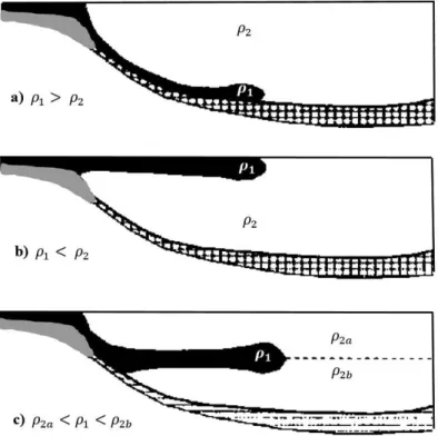
Figure 2.1: Schemes as example of possible density flow patterns for a gravity current
discharge into the water bodies ! intruding in the ambient fluid with uniform density" #, and #$< !< #%: a) underflow gravity current, b) overflow gravity current, and c) interflow gravity
current (Morris & Fan 1998, and Cesare et al. 2006). In this study:"" ! = &$'()*"and" # =
+$,*-. ... 8
Figure 2.2: Structure Scheme of a bottom gravity current (Chowdhury & Testik 2014). ... 11 Figure 2.3: The mean concentration profiles found in previous literature; a) Smooth profile, b)
Stepped profile, and c) Lutocline profile [Jacobson, & Testik (2014), and Kneller& Buckee (2000)]. ... 12
Figure 2.4: The mean velocity profile of a constant-flux release two-dimensional gravity
current, the x- and y-axis values are normalized (Kneller & Buckee 2000 and Jacobson, & Testik 2013). ... 13
Figure 2.5: Schematic of flow a) a vertical positively downward discharge of the denser (than
ambient water) fluids, b) a vertical negatively upward discharge of lighter fluids, c) the angled upward negatively discharge of denser fluids and d) a horizontal positively discharge of denser fluids (Papakonstantis & Christodoulou 2010 and Chowdhury & Testik 2014). ... 15
Figure 2.6: The experimental measurements and proposed fits of the dependency of
entrainment on Richardson number [Johnson & Hogg (2013) compared their results with those of Christodoulou (1986), Parker et al. (1987) and Ross et al. (2006)]. ... 26
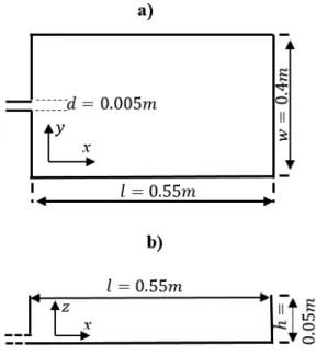
Figure 3.1: Experimental setup of the horizontal miscible jet. ... 37 Figure 3.2: Definition sketch of the basin used to perform 3D injection experiment: (a) top
view; and (b) side view. ... 38
Figure 3.3: Overview of ImageJ software. ... 40 Figure 3.4: The steps of profile result realization for R=2778: (a) the source of images series
without motion ./0123 (b) the first image ./0143 at t=0, (c) the Difference result of images series; Difference:"/012 = /012 5 /014, (d) the image after applying the adjust brightness/contrast at t=2s, (e) the binary image at t=2s, and (f) the skeletonized image at t=2s. ... 42
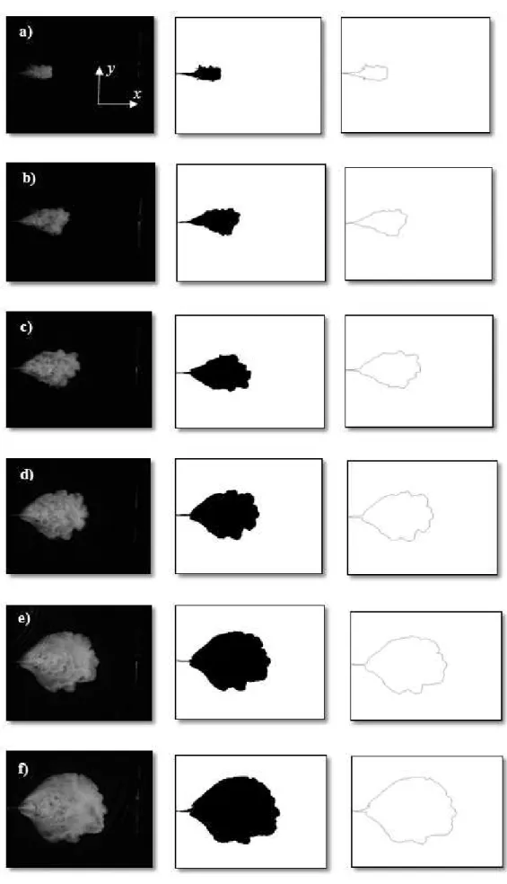
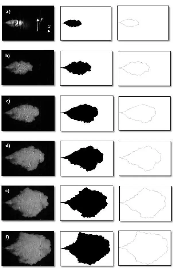
Figure 3.5: Experimental frames captured by difference (row 1), made binary (row 2), and
skeletonize (row 3) processes of two dimensional gravity currents performed with initial density " & = 2676" 81 0: 9 and +$,*- = 2666 81 0: 9" for R=1111, and frames acquired at (a) t= 2s,
(b) t=4s, (c) t=6s, (d) t=8s, (e) t=10s, and (f) t=12s. ... 44
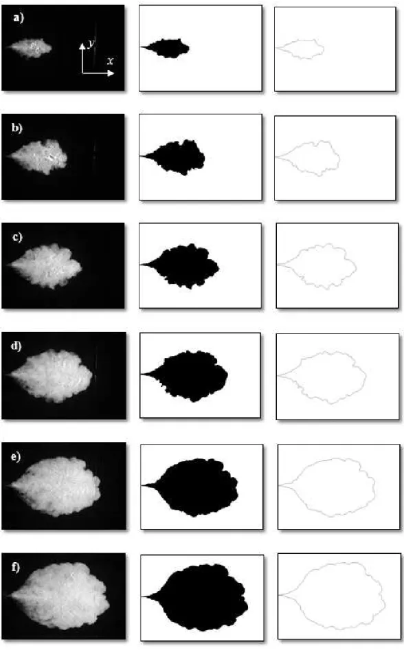
Figure 3.6: Experimental frames captured by difference (row 1), made binary (row 2), and
skeletonize (row 3) processes of two dimensional gravity currents performed with initial density " & = 2676" 81 0: 9and !"#$% = 1000 &' (* )for R=1667, and frames acquired at (a) t= 2s,
(b) t=4s, (c) t=6s, (d) t=8s, (e) t=10s, and (f) t=12s. ... 45
Figure 3.7: Experimental frames captured by difference (row 1), made binary (row 2), and
skeletonize (row 3) processes of two dimensional gravity currents performed with initial density + , = 1040+ &' (* )and
!"#$% = 1000 &' (* )for R=2222, and frames acquired at (a) t= 2s,
(b) t=4s, (c) t=6s, (d) t=8s, (e) t=10s, and (f) t=12s. ... 46
Figure 3.8: Experimental frames captured by difference (row 1), made binary (row 2), and
! = 1040! "# $& %and'()*+, = 1000 "# $& %! for R=2778, and frames acquired at (a) t= 2s,
(b) t=4s, (c) t=6s, (d) t=8s, (e) t=10s, and (f) t=12s. ... 47
Figure 3.9: Experimental frames captured by difference (row 1), made binary (row 2), and skeletonize (row 3) processes of two dimensional gravity currents performed with initial density !!' = 1040! "# $& %and'()*+, = 1000 "# $& % for R=3333, and frames acquired at (a) t= 2s, (b) t=4s, (c) t=6s, (d) t=8s, (e) t=10s, and (f) t=12s. ... 48
Figure 3.10: Experimental frames captured by difference (row 1), made binary (row 2), and skeletonize processes (row 3) of two dimensional gravity currents performed with initial density !' = 1040! "# $& %and '()*+, = 1000 "# $& %for R=3889, and frames acquired at (a) t= 2s, (b) t=4s, (c) t=6s, (d) t=8s, (e) t=10s, and (f) t=12s. ... 49
Figure 3.11: Original Frames capturing of two-dimensional gravity currents performed with initial density !!' = 1040! "# $& % and '()*+, = 1000 "# $& % for R=2778, and frames acquired at (a) t= 2s, (b) t=4s, (c) t=6s, (d) t=8s, (e) t=10s, (f) t=12s. ... 50
Figure 3.12: Dimensional characteristics of salt gravity currents front position versus time for the x and y axes. ... 51
Figure 3.13: Experimental outer positions of the mixing gravity current at xf (y, t): a) R=2222; b) R=2778; c) R=3333; d) R=3889. ... 53
Figure 3.14: Snapshots with 2D lobes and clefts structures at the front of the intruding gravity current development over a smooth bottom for: (a) R=1111, (b) R=1667, (c) R=2222, (d) R=2778, (e) R=3333, and (f) R=3889 at t=2, 4, 6, 8, 10, and 12s respectively. ... 55
Figure 4.1: The configuration of an injection by a square channel and into fresh water basin. ... 63
Figure 4.2: Overview of OpenFOAM structure. ... 64
Figure 4.3: Scheme of the general configuration of OpenFOAM. ... 65
Figure 4.4: The meshes 3D view. ... 67
Figure 4.5: Scheme of the boundary conditions of the basin in the numerical model. ... 69
Figure 4.6: Iso-volume fraction evolution of the saline gravity current jet (x,y) with α=3% for Run6 (R=3889): a) t=0s, b) t=2s, c) t=4s, d) t=6s, e) t=8s, f) t=10s, and g) t=12s. ... 69
Figure 4.7: Numerical frames captured by difference (row 1), made binary (row 2), and skeletonize (row 3) processes of two dimensional gravity currents performed with initial density!!' = 1040! "# $& %and'()*+, = 1000 "# $& %for R=3889, and frames acquired at (a) t= 2s, (b) t=4s, (c) t=6s, (d) t=8s, (e) t=10s, and (f) t=12s. ... 70
Figure 4.8: Numerical outer positions of the mixing gravity current at xf (y, t): a) R=2222; b) R=2778; c) R=3333; d) R=3889. ... 72
Figure 4.9: Evolution of spreading with time for: a) R=1111, b) R=1667, c) R=2222, d) R=2778, e) R=3333, and f) R=3889... 73
Figure 5.1: Evolution of the experimental (left side) and numerical (right side) mixing gravity current jet from the top view (x, y) for R=3889. Experimental (left side) profiles are the treated images of light intensity recordered by the camera I(x, y) and numerical (right side) profiles are the variation of the density. ... 75
Figure 5.2: Evolution of the numerical density of the mixing gravity current jet from the side view (x, z) for R=3889: a) t=1s; b) t=5s; c) t=11 s. ... 76
Figure 5.3: a) Evolution of the light intensity of mixing gravity current obtained by the contrast difference using the Rhodamine B as function of x direction, b) Evolution of numerical density of jet as function of x direction at y=l/2; z=0.005m; t=5s for!- = 2778, and xf is the front position at y=l/2. ... 77
Figure 5.4: Experimental and numerical positions of the mixing gravity current xf as a function of time for: a) R=1111; b) R=1667; c) R=2222; d) R=2778; e) R=3333; and f) R=3889. ... 78
Figure 5.5: Experimental and numerical continuous of the mixing gravity current xf (y, t): a) R=2222; b) R=2778; c) R=3333; and d) R=3889. ... 79
Figure 5.7: Dimensionless mean horizontal velocity profile versus the vertical coordinate 0.5
at ! = "/2. ... 81
Figure 5.8: Dimensionless mean excess-density profiles in the (x, z) plane at ! = "/2. ... 82
Figure 5.9: Dimensionless mean excess-density profiles. ... 82
Figure 5.10: Dimensionless mean excess-density profiles in the (y, z) plane at: a) x/d=20 and b) x/d=50. ... 83
Figure 5.11: Profiles of the excess-density and velocity in y-coordinate at: a) x/d=20, x/d=50. ... 84
Figure 5.12: Gradient Richardson number profiles indicating the increase in stable stratification with downstream distance for x/d>xmax/d where xmax/d=50 for R=3889 (run 6). 85 Figure 5.13: Position of Gradient Richadson number #$% at 0.25 in the (y,z) plane for different position from the inlet x/d. a, b, c, d, e, f, g, h, i and k represent the position from the inlet respectively for 8, 15, 20, 25, 30, 35, 40, 45, 55 and 60. ... 86
Figure 5.14: Iso-density evolution of the gravity current jet with α=3% for Run6 (R=3889): a) t=1s, b) t=5s; c) t=11s. ... 87
Figure 5.15: Evolution of the volume fraction of salt water with time with α=3% for Run6 (R=3889): a) 1s; b) 4s; c) 8s; d) 10s; and e) 12s. ... 88
Figure 5.16: The fractional volume &/&' of total volume to the initial injection volume of the fluid current plotted as a function of the front position run3. ... 89
Figure 5.17: Fraction volume &/&' of total volume to the initial injection volume of the fluid current plotted as a function of the front position for: a) run4, b) run5, and c) run6. ... 90
Figure 5.18: Fraction volume &/&' of total volume to the initial injection volume of the fluid current for different concentrations threshold plotted as a function of position front: a) 3%, b) 20%, c) 35%, d) 45%, e) 55%, and f) 65%. ... 91
Figure A.1: A plot of the gravity current flow and co-ordinate system. ... 97
Figure A.2: Two transversal cross section view element ... 99
Figure A.3: A plot of the inclined gravity current flow. ... 101
Figure A.4: A plot of the inclined gravity current flow and co-ordinate system. ... 102
Figure A.5: A plot of the inclined frontal gravity current head flow and co-ordinate system. ... 103
Figure A.6: A plot of pressure field the inclined gravity current in the ambient fluid. ... 104
LIST OF TABLES
Table 3.1: Inlet experimental control parameters conditions (x/d=0) with Sc=667 and ()* = 0.39+ , -4 1 ... 40Table 3.2: Scaling laws for two dimensions gravity currents:+6 = 78:;< and+! = 78:;. ... 52
Table 4.1: The values of the empirical constants in the high Reynolds number of > ? @ model. ... 59
Table 4.2: Inlet conditions (6 A4 = 0) with Sc=667 and ()* = 0.39 , -4 1. ... 61
Table 4.3: Boundary conditions. ... 63
Table 4.4: Positions of physical properties of OpenFOAM. ... 66
ACRONYMS
CFD Computational Fluid Dynamics
CFM2015 22ème Congrès Français de Mécanique
DNS Direct Numerical Simulation
FLUVISU2015 16ème colloque français sur la Visualisation et le Traitement d’Images en
Mécanique des Fluides
ICCOE 2016 The 2016 3rd International Conference on Coastal and Ocean Engineering
ic-rmm2-2015 2nd International Conference on Rheology and Modelling of Materials
IJET International Journal of Engineering and Technology
JWARP Journal of Water Resource and Protection
LES Large Eddy Simulation
LS-PIV Large Scale-Particle Image Velocimetry
MTT1956 Morton-Taylor-Turner
ODE Ordinary Differential Equation
PDE Partial Differential Equation
PIV Particle Image Velocimetry
PSFVIP10 10th Pacific Symposium on Flow Visualization and Image Processing Conference
RANS Reynolds-Averaged Navier-Stokes
LIST OF SYMBOLS
Symbol Definition Units
surface tension coefficient /!
" density of gravity current jet #$/!%
& molecular kinematic viscosity m2/s
' viscosity !(/)
* slop angle of the basin bottom °
+ dissipation rate of turbulent kinetic energy !(/)%
, threshold concentrations -
-" excess-density of the mixing #$/!%
.0 initial vertical velocity component m/s
10 initial dense fluid injection velocity (or 23) m/s
4 time )
# turbulent kinetic energy !(/)(
$ magnitude of gravity acceleration !/)(
5 initial depth of the dense fluid channel jet m
6 volume of gravity current at defined threshold concentration , !%
78 Schmidt number -
9: bulk Richardson number (or 9:;) -
9 initial Reynolds number (or 9<3) -
=0 initial dense flow rate !%/)
> length of experimental basin (?@) !
A depth of ambient fluid (?B) or (A3) !
CD initial Froude number (or CD3) -
z vertical spatial coordinate
y lateral spatial coordinate
x streamwise spatial coordinate
w width of experimental basin (!") m
u mean horizontal velocity /#
P pressure $ & %
' inlet depth of the gravity current jet (( = !))
*+ difference between mean velocities of both denser and return currents
/#
, fractional height -
-. momentum diffusivity m
2/s
0) initial lateral velocity component /#
123456 density of fresh water 78/
9
1: density of salt water 78/
9
;4 turbulent kinematic viscosity
%& #
<23456 water viscosity
%/#
<4 effective dynamic turbulence viscosity m
2/s
<: saline fluid turbulence viscosity
%/#
<5.. effective viscosity
%/#
>) discharge angle to the horizontal °
?) initial dissipation rate
%/#9
@. final terminal height of rise (refers to upper jet boundary)
@)AB height of half the maximum streamwise velocity
@C vertical distance of the source-bottom separation from the nozzle
D. streamwise front position of the gravity current (or E.) m
duration (time) of the wall jet phase !
"# certain time !
$% initial turbulent kinetic energy &'/!'
()* impingement visual acceleration of gravity &/!'
+ radial extent/length of the wall-jet &
+), distance from the source and impinges at an angle -to the horizontal &
.% volume of saline water injected &0
1) initial dense fluid injection velocity m/s
2) interface point &
234 turbulence Schmidt number -
567 gradient Richardson number -
8) impingement dense flow rate &0/!
9:4, atmospheric pressure ; &< '
;' buoyancy frequency !='
>) impingement momentum flux &?<!'
>% initial momentum flux (mass flux) &?<!'
@A source length scale &
@B momentum jet length scale &
C, mass molecular (diffusivity) of the injected saline fluid &'/!
DEF dissipation rate empirical constant -
DEG turbulent kinetic energy empirical constant -
DH turbulent viscosity empirical constant -
I) impingement buoyancy flux &?/!0
I% initial buoyancy flux &?/!0
!" outlet boundary condition -
#$% inlet boundary condition -
&$ impingement depth '
&( non-constant depth '
)*+,- maximum mean excess density ./0'1
/23 initial visual acceleration of gravity at the injection source ' 46 5
7 frequency of the buoyancy oscillation (Brunt–Väisälä frequency) 8 46
9 characteristic velocity ' 46
:; entrainment of the tail -
<=> entrainment velocity into the tail (or <?) ' 46
)@ growing in transport of the density current over the length of the tail '
56 4
l length of the tail section '
:A entrainment in the head -
E total entrainment quantitively of ambient fluid into gravity current -
B" ",C total area of dense fluid '
5
B2 total area that has entered the domain '
5
D+,- maximum rise of the plume height '
<?$ bulk entrainment at high Richardson number -
E?$ bulk entrainment discharge '
16 4
:,F :GF :H total, background, and potential energies
Introduction
1.1 Gravity currents
The subject of this dissertation is Experimental and Numerical study of Model Gravity currents in Coastal Environment “Bottom Gravity Currents”. Gravity currents, sometimes called density currents or buoyancy currents, are flows generated by a density gradient between two fluids and occur in both natural and industrial flows. The density differences can be due to the variations in salinity, temperature, or concentration of suspended particulates (Benjamin 1968, and Simpson 1997). The flow of a gravity current is predominantly horizontal. It can occur as either a top or bottom boundary current, or as an intrusion at some intermediate level. The spreading of one fluid into another fluid of a lower density, due to the horizontal density difference, is significant for many geophysical and industrial applications. Natural examples include sea breezes, avalanches (Allen 1982), estuaries (where fresh water meets salt water), surges from volcanoes, thunderstorm outflows, and sand storms (Bagnold 1941). Man-made examples include the accidental release into the atmosphere of dense gasses, early stages of an oil spillage (Kubat et al. 1998), etc. They can be either toxic or poisonous. Fig. 1.1 shows some examples of cases cited earlier.
In his theoretical work, Von Kàrmàn (1940) proposed a perfect-fluid model for steadily gravity currents propagation as a first calculation. Also, he used an inviscid analysis to predict the front speed and interface shape of a gravity current flowing under an infinite ambient fluid. Von Kàrmàn’s (1940) work was updated by Benjamin (1968). In Simpson’s (1997) book a comprehensive description of gravity current flows in both environmental and laboratory fields can be found. Huppert (2006), and Ungarish (2009) give excellent reviews on the conceptual foundations used to understand and evaluate the evolution of gravity currents. Bottom and free-surface gravity currents are produced by a multitude of municipal, agricultural, domestic, and industrial fluid buoyant jet discharge operations. These currents are a vital source of environmental concerns in that they present a typically adverse effect on the water quality, underwater flora and fauna, and the benthic environment. For example, bottom gravity currents generated by the buoyant sediment-laden jet disposal in coastal dredging and disposal operations can significantly affect the surrounding aquatic environment (Nichols & Thompson 1978, and Hales 1996). Because of the density difference between fluids produced by dissolved substances (i.e. salt), the current is conservative since the total mass of the dissolved substance is conserved. Variations in density in such currents are only due to entrainment of ambient fluid (Nogueira 2013c).
The turbidity currents, which are sediment-laden underflows driven by a density difference between the ambient fluid and saline density currents, are examples of gravity currents. The driving buoyancy forces are simply due to the presence of suspended particles getting a turbidity current. The lower current, which is formed inside an intrusive turbidity gravity current at some neutrally buoyant intermediate depth, depends upon the volume fraction of both fluids. Furthermore, particle settling can lead to complete buoyancy reversal, the initiation of a buoyant plume, and the subsequent creation of a surface gravity current in which the few remaining particles play no role in the dynamics of the flow (Montgomery & Moodie 1999).
Figure 1.1 : Examples of gravity currents in the environment: (a) Treatment wastewaters are rejected in the St. Lawrence River (Montréal). (b) A plume of acidic aluminum-rich water in the Manning River (Australia). (c) and (d) Sand storms are examples of buoyancy driven gravity currents in the atmosphere of specific interest is how ground friction affects speed of propagation and mixing in gravity currents in Iraq, 2015. (e) Gravity currents, in the form of pyroclastic flows, propagate down the flanks of the volcano in Mayon, Philippines, 1984. And (f) avalanche from Hunza Peak, Karimabad, in Pakistan. a) b) c) d) e) f) https://bateausportquebec.forumsactifs.com/t213 8p1sentir-la-marde https://fishhabitat.org.au/about-fish-habitat http://www.dailymail.co.uk/news/article-3097168 http://www.dailymail.co.uk/news/article-3097168 http://blankonthemap.free.fr/95_update/info038_ang.htm https://volcanoes.usgs.gov/Imgs/Jpg/Mayon/32923351-020_caption.html
1.2 Statement of the problem
Various municipal, agricultural, domestic, and industrial liquid discharge into lakes, estuaries, reservoirs, rivers, seas, and oceans. Most waste water, heated water from power plants, brine slurry from desalination plants, and dredged mud slurry are routinely released both intentionally and accidentally. In many of these operations, the discharges occur through a submerged round outfall into the receiving waters. The gravity currents were investigated in a 2D configuration experimentally and numerically in several previous works (e.g. Turner 1973, Simpson & Britter 1979, Huppert & Simpson 1980, Rottman & Simpson 1983, Hallworth et al. 1993 & 1996, Winter et al. 1995, Hacker et al. 1996, Shin et al. 2004, Lowe et al. 2005, Ungarish 2007, and 2009, Nogueira et al. 2013a, Fragoso 2013, among others). There are only few studies devoted to the 3D mixing gravity current (Ӧzgökmen et al. 2004a, Chang et al. 2005, Ilicak 2014, and Ottolenghi et al. 2016a, b & 2017).
The primary motivation behind this work in my dissertation is a study of both 2D and 3D dense bottom gravity currents propagation on a smooth bed, experimentally and numerically respectively. Also, it provides fundamental knowledge for the flow characteristics of the environmental impacts associated with the dense gravity current phenomenon. To our best knowledge, studies focusing on the mixing of the gravity flow in 3D jet configurations for the weak turbulent regime are very few. Notably, in all these studies cited previously, four key issues were not addressed: i) the dynamics of a 3D gravity current jet, ii) the hydrodynamic and density distributions of a 3D gravity current jet, iii) the turbulent mixing in a 3D gravity current jet for the weak turbulent regime, and iv) the entrainment of a 3D mixing gravity current jet.
These four issues contribute to the internal structuration of the spatiotemporal evolution of a 3D density current in a miscible ambient fluid. Fulfilling that gap constitutes the motivation of the present work. In this dissertation, RANS with k-ε and diffusion-convection equations were used to model the 3D propagation and mixing of a saline gravity current into the ambient fresh water over a smooth horizontal bottom. The dynamics of the gravity current obtained by that numerical model and experimental studies present a good agreement. The Reynolds number R and the Richardson number Ri vary in the intervals [2222, 3889] and [0.003, 0.01] respectively. The mean flow profiles of the velocity and density obtained by the numerical simulations are used to calculate the gradient Richardson number !" with the distance from
the inlet. The spatial evolution of !"#can give the turbulent mixing zone following the criterion
value of Turner (1973). The entrainment estimates the characterization of the mixing process at different values of the iso-density threshold with the front position.
1.3 Methodology
In our example of gravity currents, such as the spreading of a dense gravity current jet, the flow over the smooth bottom of the calm ambient fluid is turbulent. Small scale mixing processes between the ambient fluid and the dense fluid, due to turbulence, are important to the dynamics of the flow. As a result of the complication of the flow in a gravity current, it is difficult to understand the flow development. There are several approaches which can be used to solve this problem. The first approach is the state of the art, in order to develop a comprehensive look of the bottom gravity currents moving forward with front velocity. The resulting gravity current propagation calculation were deduced from experimental studies. The gravity current head was neglected because is very small and very difficult for Newtonian gravity currents to handle. Furthermore, investigations of the horizontal injection gravity currents propagation were presented in the state of the art.
The second approach for studying problems involving gravity currents, which complements the bibliography work, is the use of experiments. These can be small scale jet gravity currents experiments in the laboratory. The experiments or measurements of jet flows, include all the details of the flow and can be used to obtain values for experimental parameters in the numerical model, as well as checking if the model gives reasonable predictions. Experiments are the only means to provide a full study of the weak turbulent high Reynolds number flows.
The third approach which is numerical, aims at characterizing the mixing of fresh and saline waters by applying the Reynolds-Averaged Navier-Stokes equations (RANS), K-epsilon (k-ε) and the Diffusion-Convective equation (DCE) of the volume fraction. It also compares the mean flow profiles by RANS with measurement results, and calculates the Richardson number !" as a factor representing the turbulent mixing zone. Consequently, this third approach
examines the effects of volume ratio with time, as well as the quantity and the concentrations of mixed fluid produced leading to entrainment as a function of threshold with time were investigated. The use of simple scaling arguments for the bulk motion of the fluid gives some insight into the physical processes involved in the jet flow.
The two-dimensional gravity currents experiments play a valuable role with the three-dimensional gravity currents numerical model, and often give a good agreement in the x-axis and y-axis. Mixing is generally included through some form of parameterization, but it is currently limited to moderate Reynolds numbers by the computational requirements.
1.4 Outline of dissertation
The dissertation is organized in six chapters and two appendices. In this chapter, an introduction to gravity currents was provided, where the main motivation and objectives of this work were presented. Chapter 2 provides a review of the previous literature and the main contributions to date on bottom gravity currents. Specific topics are covered by this dissertation, and important experimental, theoretical, and numerical results are described. In Chapter 3, the use and applicability of laboratory experiments to saline gravity current jet flow over a rigid, and smooth horizontal bottom into the lighter fluid is discussed. The different experimental apparatus, techniques, and image processing used in this work are described in detail, as well as comparison between results of experiments.
In Chapter 4, a numerical model for the flow of the saline gravity current jet into the ambient fresh water in a basin and axisymmetric gravity currents is developed. The Reynolds-Averaged Navier-Stokes (RANS) and the diffusion-convection equation of the volume fraction of the saline water are used to model the mixing and the propagation of the saline gravity current. Chapter 5 presents the main results arising from the experimental measurements and numerical computations of the numerical model, then validated by comparing the predictions with the experimental results. In Chapter 6, the main conclusions of the present research are drawn and suggestions and recommendations for future works are given.
Two appendices are included at the end of the dissertation, complementing the information presented in Chapters 3, 4, and 5. Appendix A representing the development of Huppert's theory: solution of Newtonian gravity current equations, whereas Appendix B includes the equations relating to the solution of non-Newtonian gravity current (Rheology). Two solutions give additional details of the equations relating to the bottom gravity current beneath a static water layer at rest in the horizontal and inclined basin
.
1.5 Original contributions
A number of contributions emerged during these four years of research, either by papers published (or submitted) in peer-reviewed journals or by papers published in conference proceedings, these are listed below:
Ø Dhafar, I. A., Latrache, N., and Nsom, B. (2015a). Applied the Large-Scale Particle Image Velocimetry Technique for Measurement the Velocity of Gravity Currents in the Laboratory. DOI: 10.4236/jwarp.2015.78048, Journal of Water Resource and Protection 07(08):597-604.
Ø Dhafar, I., A., Latrache, N., and Nsom, B. (2015b). Image processing applied to characterize the denser gravity current propagates over rigid surface into the lighter fluid. 10th Pacific Symposium on Flow Visualization and Image Processing Conference, Naples, Italy, 15-18 June.
Ø Dhafar, I. A., Latrache, N., Niang, P., and Nsom, B. (2015c). Etalement d'un jet horizontal miscible de flottabilité positive. 22ème Congrès Français de Mécanique, Lyon, France, 24 au 28 Août.
Ø Dhafar, I. A., Nsom, B. and Latrache, N., (2015d). Effect of slope change on the dynamics of pseudoplastic mass movements beneath a static volume of water, ic-rmm2- 2 nd International Conference on Rheology and Modelling of Materials, Miskolc-Lillafüred, Hungary, 5-9, October.
Ø A prize of Doctoral School of Marine Sciences (EDSM) worth 1300 € by my presentation of the poster entitled: Experimental and Numerical Study of Model Gravity Currents in Coastal Environment. The days of the Doctoral School of Marine Sciences (EDSM) were held on 5 and 6 November 2015e.
Ø Dhafar, I. A., Latrache, N., and Nsom, B. (2015f). Mesure de vitesse par PIV à grande échelle d’un écoulement de courant gravitaire d’un liquide léger à la surface libre d’un liquide dense. 16ème congrès français du Club FLUVISU (« Visualisation et Traitements d’images en Mécaniques des Fluides pour l’Industrie »), associé au 14ème colloque international francophone du Club CMOI (« Contrôles et Mesures Optiques pour l’Industrie»). Lannion, France, Du 16 au 20 novembre.
Ø Dhafar, I. A., Latrache, N., and Nsom, B. (2016). Experimental Study of the Effect of the Spreading Buoyant Gravity Current on the Coastal Environment. The 2016 3rd International Conference on Coastal and Ocean Engineering (ICCOE 2016), Tokyo, Japan, 8-9, April.
Ø Dhafar, I. A., Latrache, N., and Nsom, B. (2017a). Experimental Study of the Effect of the Spreading Buoyant Gravity Current on the Coastal Environment. DOI: 10.7763/IJET.2017.V9.957. International Journal of Engineering and Technology, 09(02):129-132.
Ø Dhafar, I. A., Latrache, N., and Nsom, B. (2017b). Mixing of Saline gravity Current Jet into Fresh Water in the Weakly Turbulent Regime (under review).
Literature Review
Many studies investigated gravity currents using both laboratory experiments and numerical simulations. The aim of this chapter is to provide a review of some literature centered on gravity currents that are relevant to this dissertation, and specifically related to the dense gravity current phenomenon. As discussed in Chapter 1, various municipal, agricultural, domestic, and industrial liquid discharge in the sea or ocean incredibly cause adverse environmental impacts via the formation of gravity currents. In section 2.1, the classification of gravity currents, then, the structure of the bottom gravity currents in section 2.2 are summarized. Section 2.3 presents the dispersion characteristics of buoyant gravity current jet discharges. Entrainment and mixing gravity currents are described in section 2.4, while the section 2.5 includes the numerical modeling. The discussion is mostly focused on the process of interest of this investigation “bottom gravity currents”. However, many of the concepts, results, and conclusions of studies concentrate on a gravity current flow composed of a different medium are advantageous in this analysis.
2.1 Classification of gravity currents
A gravity current is a flow of a fluid with density !within an ambient fluid of different
density," #. The density gradient between fluids in such currents is primarily horizontal. The
flows generated by vertical density gradients as a plumes are not within the scope of the present study. According to the different density types of the current and the ambient fluid, gravity currents can be classified as bottom currents (Fig. 2.1), when the current is denser than the ambient fluid, !> #; top currents, if the density of the current is lower than the ambient fluid, !< #; or intermediate currents, when the current has intermediate density value when
compared to the stratified ambient fluid, #$< !<" #%. The total depth of the two fluids is H,
and non-constant depth h* moves forward with front velocity ! into the surrounding fluid with the lower density"#. Moreover, gravity currents can be categorized as compositional or particle-driven gravity currents. In the case of compositional gravity currents, the driving force appears in dissolved solute like salt in the sea or difference of temperature. While for particle-driven gravity currents, the driving force is represented by the suspension of sediments. In a compositional gravity current, the current is conservative since the total mass of the dissolved substance is conserved. Variations in density in such currents are only due to entrainment of the$"%, "# ambient fluid.
Figure 2.1: Schemes as example of possible density flow patterns for a gravity current discharge into the water bodies !"intruding in the ambient fluid with uniform density #, and #$< !< #%: a) underflow gravity current, b) overflow gravity current, and c) interflow gravity current (Morris & Fan 1998, and Cesare et al. 2006). In this study: !"= !#$%&'( and !)= !*$+(,.
Gravity currents, of a high Reynolds number flow rate, are unsteady, turbulent, and tend to entrain ambient fluid. For instance, when gravity currents can entrain particles from the bed and deposit suspended material, changing the total amount of particles in the flow. The results of such entrainment, and the resulting dilution of the original intruding fluid, can be quite important. For example, many industrial pollutants are discharged into the atmosphere or hydrosphere with a contrasting density to their ambient surroundings. The dilution with distance of any resulting gravity currents by entrainment has important implications for toxicity levels and the degree and extent of contamination (Hallworth et al. 1993 &1995). In the following, a summary for relevant bottom gravity current classifications related to this dissertion, will be presented. The dynamics of gravity current jets are developed following different phases: the first phase is the balance between the radial momentum flux and the rate of change of the inertial force and is characterized by a constant speed front (Chen, 1980). While the second phase (inertia regime) is characterized by the equilibrium between inertia and buoyancy forces, and the third phase (viscous regime) by the equilibrium between viscous and buoyancy forces (Hoult, 1972, Huppert & Simpson 1980, and Huppert 1982). The internal flow structure of density currents is a key issue for understanding the spatiotemporal evolution of the mixing or entrainment of the ambient fluid into the head of the current during its propagation.
2.1.1
Density ratio of current to ambient fluids
Benjamin (1968), Rottman & Simpson (1983), Haertel et al. (2000), Marino et al. (2005), and Ungarish & Zemach (2005) discussed the term of Boussinesq flows, which correspond to a small density difference between fluids. The density difference is mostly driving a high flow of the initial density jumping across the interface. The differences in the structure and shape of a gravity current depend on the ratio of initial density between the dense and the light fluids. When the two fluids densities are comparable (approximately equal), the progress of the gravity current helps understanding the presence of the ambient fluid, which imposes a significant resistive force on the intruding current. However, Birman et al. (2005), Etienne et al. (2005), Lowe et al. (2005), Ungarish (2007), and Bonometti et al. (2008) focused of the cases in which the current density is much higher than the ambient one. In the case of a dam break flow in which water spreads in the air, the current is not affected by any resistance from the surrounding ambient. Typically, the density difference is small enough for the Boussinesq approximation to be valid. The Boussinesq approximation is applied to problems where the fluid varies in temperature from one place to another, driving a flow of fluid and heat transfer. The Boussinesq gravity current acquires shape with a head, and a body as shown in (§2.2-Fig.2.2), while the thickness of a non-Boussinesq current decreases monotonically while approaching the ambient fluid, reaching a minimal value at the front of the current. Also, the current acquires a final height at which the flow is reversed, and returns to the bottom where it spreads as a gravity current. The brines produced from the desolation process are usually discharge into coastal waters as an example of denser current injection into lighter ambient.
2.1.2
Density difference of current and ambient fluids
The difference in density between the gravity current and ambient fluids is due to temperature, concentration, or compositional (different fluids completely) variations, or as an outcome of particles suspended. Bonnecaze et al. (1993), Hallworth & Huppert (1998), Gladstone et al. (1998), and Necker et al. (2002) characterized the case of a particle-laden current. Fresh water (lighter fluid) exits from a river into the ocean (dense liquid), it flows along the surface, partially due to the difference in salinity between fresh and saline water as shown in Fig. 2.1b. The turbid mixture spreading on the seafloor represents an example where the excess density in the current comes about from the suspension of sediments as shown in Fig. 2.1a. In a non-mixing case, the density of a particle-laden current continues to develop in space and time as a result of the continuous deposition of particles and possible re-entrainment back into the flow (if the current is energetic enough).
2.1.3
Continuous release with finite volume
Simpson (1972), Huppert & Simpson (1980), Bonnecaze et al. (1995), Hacker et al. (1996), Gladstone et al. (1998), Shin et al. (2004), and Cantero et al. (2007a) described the gravity current as a finite release. Following their description, a fixed volume of fluid is suddenly discharged into an ambient environment of a different density. Whereas Garcia & Parker (1993), Hogg et al. (2005), Sequeiros et al. (2009), and Shringarpure et al. (2012) described a continuous release. Based on the source configuration, there are two major types of gravity currents: constant-volume (or fixed-buoyancy) and continuous-flux (or continuous-buoyancy). Constant-volume gravity currents are generated in the laboratory through the use of a lock-exchange tank (Chowdhury & Testik 2014). As a rule, the current release is produced from a large tank with a time-dependent flux q as = !"!, where ! is a positive constant, " is the time of positions, and # is an exponent either positive (waxing release), negative (waning release) or null (fixed, limited volume release). The limited release is observed when the sides of a container suddenly collapses releasing the embodied fluid instantaneously, while a continuous release can be the consequence of a small rupture along one of the edges of a large container or a pipeline leading to a continuous discharge of material. The fluid spreading due to a constant source of buoyancy on the surface or the bottom of a calm ambient was investigated experimentally and theoretically. Britter (1979), Chen (1980), Didden & Maxworthy (1982), Huppert (1982), and Lister & Kerr (1989) provided the estimation equations of the axisymmetric gravity current radius as a function of time, and source flow parameters (see §§2.3.1).
2.1.4
Geometrical limitations
In general, the gravity currents are studied in one of two geometric constraints, in particular the planner and the axisymmetric setups. These configurations are widely searched due to their simplicity on the contrary of my dissertation case. Experimental and numerical studies provide an easily construct and a more flexible challenge for modeling aims (Shallow Water equations and Box Model). The planar release case, a flat rectangular gate at first separates a rectangular reservoir of fluid from an ambient with lower density. As well, at the start of the axisymmetric three-dimensional release case, the current is confined inside a hollow circular cylinder at the center of a large tank containing the ambient fluid (Huppert 1982, and Cantero et al. 2007b). Huppert & Simpson (1980), and Cantero et al. (2007a) was investigated the small angle of expansion typically 10-15° by an expanding inside the tank.
The gate would be partially lifted up, and the restricted fluid would be continuously fed to maintain the desired volumetric discharge rate as a continuous release. The setup of the planar case used of as a two-dimensional releasing since the current is confined to move in a specified direction. While for the set-up of the circular discharge case, the current would spread radially outwards (in all directions) but remains axisymmetric because of the fundamental circular nature of the release.
2.2 Bottom gravity currents structure
Bottom gravity currents are formed by a head region at the front, which is usually deeper than the following tail. It advances into the ambient fluid and it is followed by the body or sometimes a tail (Kneller & Buckee, 2000). Although some mixing usually occurs at the head, the clear distinction between the gravity current and the ambient fluid typically remains. During propagation, the mass and momentum balance in the head differs significantly from in the body (Middleton 1993). The head must displace the stationary ambient water resulting in a greater thickness than the trailing body. As shown in Fig.2.2, a cross-section of 2D gravity current
along a horizontal bottom surface, generated by a constant buoyancy flux ‘constant-volume
release’ (see §§ 2.1.3) at the left end could be considered. It propagates with a distinct dividing line making a body, a head or/and a front.
Figure 2.2: Structure Scheme of a bottom gravity current (Chowdhury & Testik 2014).
Generally, the front part of this current, which is deeper/thicker than the body, is known as the head of the gravity current (Britter & Simpson 1978). The symbols: S represents the particle erosion from the bottom, D particle deposition from the gravity current, !velocity of the front,
"# entrainment velocity into the current, $% density of the current, and $& density of the ambient
water (Chowdhury & Testik 2014). The frontal zone of a propagating saline gravity current had been investigated in a number of previous studies (e.g. Simpson 1969, Fleischmann et al. 1994, Härtel et al. 2000a & b, La Rocca et al. 2008, and Ottolenghi et al. 2016a, b & 2017). The following sections focus on the structure of the bottom gravity currents propagation over a horizontal bed.
2.2.1
Distribution of bottom gravity current concentration
For a Newtonian fluid, the experimental measurements of concentration profiles revealed the existence of two main types. For constant-flux release-inertial gravity currents: the smooth profile and the stepped profile are shown in Fig. 2.3a and b respectively (Chowdhury & Testik 2014). In one of the earlier studies on gravity currents, Ellison & Turner (1959) studied concentration profiles in constant flux gravity currents as shown in Fig.2.3a. They observed a decline concentration gradient near the bottom boundary that fell off rapidly near the height of the velocity maximum. Garcia (1993 & 1994) found a layer of nearly constant density extending up to the velocity maximum then decreasing dramatically in the vertical direction as shown in Fig.2.3b. While, for a non-Newtonian fluid, Van Kessel & Kranenburg (1996) observed a lutocline profile for high concentration fluid of mud gravity currents which they attributed to the Bingham rheology of the liquid mud as shown in Fig2.3c. It is similar to the stepped profile presented in Fig.2.3b.
Figure 2.3: The mean concentration profiles found in previous literature; a) Smooth profile, b) Stepped profile, and c) Lutocline profile [Jacobson & Testik (2014) and Kneller& Buckee (2000)].
Three-Dimensional unsteady flow characterizes the gravity current head. Two types of turbulence structures of instability which govern the mixing processes are the Kelvin- Helmholtz instability on the one hand and lobes and clefts on the other hand (Simpson 1969, 1972, 1997, Allen 1971, Britter & Simpson 1978, Chowdhury et al. 2009, and Peng & Lee 2010). Kelvin-Helmholtz billow (wave) are generated in the interfacial region, at the rear of the current head, and roll up as the current advances. They remain quasi-steady in the current body, disappearing away due to continuous mixing with the surrounding fluid. Lobes and clefts produced by a convective instability formed at the first region of the head, are caused by the incorporation of less dense fluid by the current head during its propagation which is a direct result of the no-slip boundary condition at the bottom boundary such as a rigid surface.
2.2.2
Distribution of the velocity in a bottom gravity current
The general form of the mean velocity profile in a typical inertial gravity current flow consists of a thinner inner region (near-basin wall) and a thicker outer region, both regions are separated by the maximum velocity as shown in Fig.2.4. The inner region has a positive velocity gradient and behaves similarly to a conventional turbulent boundary layer. The outer area has a negative velocity gradient that acts as a shear layer. The vertical position of the velocity maximum is controlled by the ratio of drag forces at the upper interface and the lower boundary (Middleton 1993 and Chowdhury & Testik 2014).
Figure 2.4: The mean velocity profile of a constant-flux release two-dimensional gravity current, the x- and y-axis values are normalized (Kneller & Buckee 2000, and Jacobson & Testik 2013).
Prandtl theory (1952), concerns the transient phase (see §§2.4.2) following the release of dense fluid in a low surrounding fluid with lower density. Neglecting hydrostatic forces and applying the hypothesis, which formed a roll at the rear of the head of the current, does not fall backwards. He obtained the ratio of the propagation velocity to the flow velocity by the evaluation of the dynamic pressures against the front. Prandtl’s theory can be only applied to the "transient phase" during which the confluence between the two fluids occurs after opening the injection orifice partly. The roll formed at the rear of the head of the currents fell behind and entrained with the lower layer, developing a turbulent motion at the front. After this stage of development, a state of stationary propagation takes place. Then the turbulent motion is confined to the head of the current, and the ratio of the propagation velocity to the flow velocity must be 1 (Benjamin 1968).
2.3 Dispersion of discharges of buoyant gravity current jet
Buoyancy forces are the engine for gravity current propagation. These forces are in turn counterbalanced by inertia as well as resistance due to Reynolds stress and viscous drag, both acting at the upper and lower boundaries of the current. When the propagation velocity decreases, viscous stresses become significant and counterbalance buoyancy as well (Nogueira 2013c). The developed gravity currents is typically an unsteady phenomenon, i.e., the current kinematics and the internal density distribution are time varying. Many buoyant jet discharge configurations can be found. Only the four following ones, which concern our study, are presented. Firstly, the vertical positively downward discharges of denser fluids (Fig. 2.5a). Secondly, the vertical negatively upward discharges of lighter fluids (Fig. 2.5b). Thirdly, the inclined negatively upward discharges of dense fluids at an angle, ! to the horizontal (i.e., the angle between the discharge axis of the outlet and the horizontal, ! = 0 to"90°) (Fig. 2.5c). And fourthly, the discharge at an angle of a positively buoyant jet with similar source and ambient conditions (Fig.2.5d).
For the downward or upward discharges (with" ! = "90°), the descending (Fig. 2.5a) and rising (Fig. 2.5b) entrain ambient water of buoyant jets, expand in the water column, and eventually impinge on either the bottom or free-surface boundary. In the angled discharge configurations (Fig. 2.5c), the negatively buoyant jet of the dense fluids first rises to its high elevation over the port of discharge and then retreats in the water column to impinge on the lower boundary. A positively buoyant jet is caused from the impingement at an angle (Fig. 2.5d). The flow spreads initially as a short-lived wall jet before becoming a gravity current, when the impingement redirects the flow of the discharge as a radial outflow.
The flow spreads in x-axis, y- axis, and z-axis near the impingement point as a gravity current, i.e. a dense layer propagates horizontally on the bottom. The downward flow, after the location of the ultimate height, accelerates since the buoyancy now effects in the flow direction (Chen 1980, Moursi et al.1995, Kotsovinos 2000, Lawrence & Maclatchy 2001, Papakonstantis & Christodoulou 2010 and Chowdhury & Testik 2014). In laboratory experiments, gravity currents are studied by releasing a dense fluid into a lighter fluid by the lock-exchange technique or using a continuous source with a constant inflow rate such as a jet (Nogueira et al. 2014, Lombardi et al. 2015, Cenedese and Adduce 2008, and Ottolenghi et al. 2017). In 2D-flow theory, box models or shallow-water theory can describe the dynamics of the front and the height of the gravity currents (Hoult 1972, Huppert & Simpson 1980, and Huppert 1982).