HAL Id: tel-01199257
https://tel.archives-ouvertes.fr/tel-01199257v2
Submitted on 8 Jan 2019HAL is a multi-disciplinary open access archive for the deposit and dissemination of sci-entific research documents, whether they are pub-lished or not. The documents may come from teaching and research institutions in France or abroad, or from public or private research centers.
L’archive ouverte pluridisciplinaire HAL, est destinée au dépôt et à la diffusion de documents scientifiques de niveau recherche, publiés ou non, émanant des établissements d’enseignement et de recherche français ou étrangers, des laboratoires publics ou privés.
Jing Wu
To cite this version:
Jing Wu. A qualitative spatio-temporal modelling and reasoning approach for the representation of moving entities. Geography. Université de Bretagne occidentale - Brest, 2015. English. �NNT : 2015BRES0036�. �tel-01199257v2�
pour obtenir le titre de DOCTEUR DE L’UNIVERSITE DE BREST Mention : Nom de la mention
Ecole doctorale des SCIENCES de la MER
DOCTEUR DE l’UNIVERSITE DE BREST Spécialité : Géomatique
Ecole Doctorale des Sciences de la Mer
Préparée à l’Unité Mixte de recherche (n° 3634) Institut de Recherche de l’École Navale
A Qualitative Spatio-Temporal
Modelling and Reasoning
Approach for the Representation
of Moving Entities
Thèse soutenue le 14 Septembre 2015 devant le jury composé de :
Jean-Philippe BABAU
Professeur des universités, Université de Bretagne Occidentale / Examinateur
Thérèse LIBOUREL
Professeur des universités,LIRRM / Rapportrice
Sébastien MUSTIÈRE
Docteur ès sciences (HDR), COGIT / Rapporteur
Lamia BELOUAER
Docteur ès sciences, IRENAV / Examinatrice
Min DENG
Professeur, Central South University, CHINA / Co-directeur de thèse
T
HÈSE
présentée à
L
'U
NIVERSITÉ DE
B
RETAGNE
O
CCIDENTALE
pour obtenir le titre de
D
OCTEUR
DE
L
'U
NIVERSIT
É
DE
B
RETAGNE
O
CCIDENTALE
Mention Géomatique
par
Jing WU
soutenue le
14 Septembre 2015
devant la commission d’examen :
Composition du Jury
Rapporteurs : Pr. Thérèse LIBOUREL – LIRRM Dr. Sébastien MUSTIÈRE – COGIT
Examinateurs : Pr. Jean-Philippe BABAU – Université de Bretagne Occidentale Dr Lamia BELOUAER – IRENav
Co-Directeur : Pr. Christophe CLARAMUNT – IRENav
Pr. Min DENG – Central South University, CHINA
Équipe MOdélisation et Traitement des Informations Maritimes (MOTIM) Institut de Recherche de l’École Navale (EA 3634)
A Qualitative Spatio-Temporal Modelling and Reasoning
Approach for the Representation of Moving Entities
A
CKNOWLEDGMENTS
Pursuing a PhD degree has been a long journey. So much has happened and changed in my life during the last four years. Although the sorrow in my heart was so great that it almost crushed me, I am now rising from the ashes like a phoenix. I could by no means have carried out this work without the ongoing guidance, support, and friendship of many individuals. Whereas it would lead me too far to mention each name exhaustively, I would like to express my sincere gratitude to all the people that have helped me in any respect. Let me explicitly mention some of them.
I have to start by appreciating my parents, Mr. Jiping WU and Ms. Chunlan YAO,
because their role is far greater than my Doctoral degree. I am indebted to them for raising me as an independent and hopeful individual; always trusting my decisions and having faith in me. More importantly, I am thankful to them for showing me by example that will and faith are the essentials to make life better.
I wish to thank my supervisor Prof. Min DENG for his openness to discuss and explore
fresh ideas and his courage to face novel research challenges. I deeply appreciate giving me the opportunity to conduct my research in France at the IRENav.
I also owe my utmost gratitude to my supervisor Prof. Christophe CLARAMUNT for
his admirable academic guidance and for his willingness to be always available for me. I highly commend his great enthusiasm and diligence, and also his excellent research skills and abundant sense of humour which have made working with him a great pleasure.
I gratefully recognize the Research Foundation – China Scholarship Council for funding
my research in France.
Moreover, I want to extend my heartfelt thanks to all my friends – in China and in
France – for their unwavering support throughout the years. Especially for those far away,
it hasn’t always been easy to keep in touch, but I still appreciate them being there for me. Finally, special thanks to Buddha. Words cannot express how grateful I am to experience your guidance to explore the spirit world and to be a wise and happy woman.
To see a world in a grain of sand, And a heaven in a wild flower, Hold infinity in the palm of your hand, And eternity in an hour. ---- William Blake
T
ABLE OF
C
ONTENTS
Table of Contents... i
List of Figures ... v
List of Tables ... viii
INTRODUCTION ... 1
1 Problem Statement ... 2
2 Aim and Objectives... 3
3 Approach Overview ... 4
4 Contributions ... 5
5 Thesis Structure ... 6
CHAPTER I: Related Work ... 9
I.1 Introduction ... 10
I.2 Qualitative Spatial and Temporal Representations ... 10
2.1 Qualitative Topological Relations ... 11
2.2 Qualitative Orientation Relations ... 15
2.3 Qualitative Distance Relations ... 18
2.4 Qualitative Temporal Relations ... 20
I.3 Qualitative Spatio-Temporal Reasoning ... 21
3.1 Conceptual Neighbourhoods ... 22
3.2 Composition Tables ... 23
I.4 Qualitative Movement Modelling ... 25
4.1 Space + Time Approaches ... 26
4.2 Integrated Space-Time Approaches ... 28
I.6 Discussion ... 32
CHAPTER II: Movement Patterns ... 35
II.1 Introduction ... 36
II.2 Modelling Principles ... 37
2.1 Primitive DL-RE Topological Relations ... 38
2.2 Dimensionality and Cardinality ... 39
2.3 Dimension Sequence of an Ordered Set of Spatial Entities ... 40
2.4 Neighbouring Discs on Intersection Points ... 40
II.3 Boundary-based Movement Pattern between One Directed Line and a Region... 43
3.1 No Intersection ... 44
3.2 One 0-dimensional Intersection Point ... 44
3.3 One 1-dimensional Intersection Line ... 46
3.4 More than One Intersection ... 49
II.4 Orientation-based Movement Pattern between Two Directed Lines ... 52
II.5 Conclusion ... 57
CHAPTER III: Qualitative Representation of Moving Entities ... 59
III.1 Introduction ... 60
III.2 Spatio-Temporal Primitives ... 61
2.1 Temporal Primitives... 61
2.2 Topological Primitives ... 63
2.3 Distance Primitives ... 64
III.3 Towards a Region-Region Movement Representation ... 66
3.1 Movement outside a Reference Entity ... 66
3.2 Movement on the Boundary of a Reference Entity ... 67
3.3 Movement inside a Reference Entity ... 68
III.4 Towards a Trajectory-Region Movement Representation ... 71
4.1 No Intersection ... 71
4.2 One 0-dimensional Intersection Point ... 73
4.3 One 1-dimensional Intersection line ... 75
CHAPTER IV: Qualitative Reasoning on Moving Entities... 81
IV.1 Introduction ... 82
IV.2 Continuous Transitions of Movements ... 82
2.1 CND for Region-Region Movements ... 83
2.1.1 Interpreting the CND ... 84
2.1.2 Similarity between Region-Region Movements ... 86
2.2 CND for Trajectory-Region Movements ... 88
IV.3 Composition Tables ... 89
3.1 A Composition Table for Region-Region Movements ... 90
3.2 Case Studies ... 91
3.2.1 Case study 1 ... 91
3.2.2 Case study 2 ... 92
3.2.3 Case study 3 ... 94
IV.4 Conclusion ... 95
CHAPTER V: Experimental Applications ... 97
V.1 Introduction... 98
V.2 Application to Air Transportation ... 98
2.1 Analysis of Flight Trajectories ... 99
2.2 Flight Trajectory Reasoning ... 105
V.3 Application to Maritime Transportation ... 107
3.1 Maritime Trajectory Patterns ... 107
3.2 Maritime Trajectory Reasoning ... 109
V.4 Conclusion ... 110
CHAPTER VI: Conclusions & Perspectives ... 113
VI.1 Outline ... 114
VI.2 Main Research Findings ... 114
VI.3 Perspectives ... 117
APPENDIX A: Résumé étendu de la thèse... 121
A.2 Patrons de Mouvements ... 123
2.1 Principes de Modélisation ... 124
2.2 Patrons de Mouvements Orientés Frontière entre une Ligne Orientée et une Région .... 124
2.3 Patrons de Mouvements Basés sur des Relations d’Orientations entre deux Lignes Orientées ... 125
A.3 Représentation Qualitative de Mouvement d’Entités... 126
3.1 Primitives Spatio-temporelles... 126
3.2 Vers une Représentation de Mouvements Région-Région ... 127
3.3 Vers une Représentation d’une Trajectoire-Région ... 127
A.4 Raisonnement Qualitatif sur des Entités Mobiles ... 129
4.1 Transitions Continues de Mouvements ... 129
4.2 Tables de Composition ... 130
A.5 Applications Expérimentales ... 130
5.1 Application au Transport Aérien ... 130
5.2 Application au Transport Maritime ... 131
A.6 Conclusion ... 132
APPENDIX B: List of Publications ... 135
APPENDIX C: Short Curriculum Vitae ... 137
L
IST OF
F
IGURES
Figure 1 Research domains covered by the research ... 3
Figure 2 General outline of the thesis ... 7
Figure I.1 Graphic representation of the RCC calculus ... 13
Figure I.2 Cardinal directions between two points in 2D space: (a) cone-based model; (b) projection-based model; (c) projection-based model with neutral zone ... 16
Figure I.3 LR relations ... 17
Figure I.4 DRA relations ... 17
Figure I.5 OPRA2 relations ... 18
Figure I.6 Qualitative absolute distances ... 19
Figure I.7 Distance-based relations between si ... 20
Figure I.8 Thirteen temporal relations between two temporal intervals I1 and I2 ... 21
Figure I.9 CND of RCC8 (Randell et al. 1992)... 23
Figure I.10 Illustration of QTC ... 27
Figure I.11 Trajectory configurations example A(v+p+)B (Noyon et al. 2007) ... 28
Figure I.12 A region in space-time which is not continuous ... 29
Figure I.13 Two men walking along a street ... 33
Figure II.1 Representing movement by a directed line ... 37
Figure II.2 Topological configurations of two endpoints of L and a region. ... 39
Figure II.3 Dimensional intersections ... 40
Figure II.4 A neighbouring disc neigh(p) ... 41
Figure II.6 Classification of DL-RE topological relations ... 49
Figure II.7 Movement patterns representation: (a) several vessels towards or from one region; (b) one vessel moves across different regions ... 52
Figure II.8 The named primitives defined by the HBT model ... 53
Figure II.9Some Disjoint relations cannot be distinguished by HBT model... 54
Figure II.10Some Cross/touch relations cannot be distinguished by HBT model ... 54
Figure II.11 Reference system of the DOR model ... 54
Figure II.12 Body-body intersections between directed lines ... 55
Figure II.13 Examples of configurations between directed lines ... 56
Figure III.1 Temporal primitives ... 62
Figure III.2 Distance between two moving entities at continuous time instant ... 65
Figure III.3 Movement outside a reference entity ... 67
Figure III.4 Movement on the boundary of a reference entity ... 68
Figure III.5 Movement inside a reference entity ... 70
Figure III.6 Movement semantics of a man that enters a room... 70
Figure III.7 Trajectory configurations outside a reference entity ... 72
Figure III.8 Trajectory configurations inside a reference entity with no intersection ... 73
Figure III.9 Trajectory configurations with one 0-dimensional intersection point ... 75
Figure III.10 Movement configurations with one 1-dimensional intersection line ... 78
Figure III.11 Movement with respect to a region with a broad boundary ... 79
Figure III.12 Degenerated cases for region-region movement ... 80
Figure IV.1 CND for region-region movements ... 83
Figure IV.2 Continuous transitions of moving A over a larger region B ... 84
Figure IV.3 Continuous transitions of A moving over a smaller region B ... 85
Figure IV.4 Continuous transitions of A moving over a region B of equal size and shape 86 Figure IV.5 An example of region-region movements’ similarity ... 87
Figure IV.6 CND for trajectory-region movements ... 89
Figure IV.7. Relative movements between a man A, a car B and a parking lot C ... 92
Figure IV.8. Relative movements between a storm A, a boat B and a fishing area C ... 93
Figure IV.9. Relative movements between two men and the room ... 94
Figure V.1. Flight trajectory configurations ... 99
Figure V.2. Primitive trajectory configurations over the example of Ireland ... 101
Figure V.3. The sequence of motion event “PassThrough” ... 102
Figure V.4. Comparison of trajectory events ... 105
Figure V.5. Possible evolution of a flight trajectory ... 106
Figure V.6. Maritime trajectory patterns ... 109
Figure V.7. Forward trajectory patterns ... 110
Figure VI.1. Primitive movement patterns: (a) between a directed line and a region; (b) between two directed lines ... 116
Figure A.1. Mouvements élémentaires entre une ligne orientée et une région ... 125
Figure A.2. Mouvements élémentaires entre deux lignes orientées ... 126
Figure A.3. Configurations de mouvement Région-Région: (a) extérieur d’une entité de référence; (b) frontière d’une entité de référence; (c) à l’intérieur d’une entité de référence ... 128
L
IST OF
T
ABLES
Table I.1 Topological relations defined from the connection C relation (Cohn et al. 1997)
... 12
Table I.2 Composition table for RCC8 ... 25
Table II.1 Orientation-based movement patterns ... 56
Table IV.1 Conceptual distances between region-region movements... 88
Table IV.2 Composition table of region-region movements ... 91
Table IV.3 Composition table between a man A, a bus B and a parking lot C ... 92
Table IV.4 Composition table between a storm A, a boat B and a fishing area C ... 93
Table IV.5 Composition table between two men and a room ... 94
Table V.1. The number of different primitive configurations in various time intervals .. 100
Table V.2. The number of flights regarding different motion events ... 104
The research developed by this Ph.D. thesis (doctorat mention géomatique) is centered on the representation of moving entities in a qualitative way that should reflect as much as possible human cognitive capabilities. The motivation behind this research originates from the necessity to find formal and computational solutions for describing and reasoning on
objects’ movements in geographical spaces. We formalize an approach that represents
qualitative movements based on several spatio-temporal relations, and provides a series of reasoning methods to derive, describe and analyse possible movements.
This introductory chapter develops the main motivations and results of our research. Section 1 provides a brief introduction to qualitative spatio-temporal models and natural language approaches closely related to our work. The aim and objectives of our research are set out in Section 2. An overview of the approach developed is given in Section 3, while Section 4 describes our main contributions. Finally, Section 5 summarizes the structure of the thesis.
1 Problem Statement
Nowadays, many environmental and urban sciences require novel approaches for a better integration of the time dimension within Geographical Information Systems (GIS). Although current GISs have been largely applied over the past forty years (Goodchild 2009; Bhatt et al. 2011), the world cannot be represented and reproduced objectively if its representation if limited to static objects and spatial relationships. A series of spatio-temporal formalisms have been developed over the past few years for the representation of geographical data, even when only partial or imprecise information is available (Harmelen et al. 2008; Ligozat 2012; Claramunt and Stewart 2015). Such modelling approaches have contributed to the development of many contributions such as spatio-temporal representation of evolving spatial entities (Claramunt et al. 1997a; Hornsby and Egenhofer 2000; Erwig and Schneider 2002), spatio-temporal reasoning frameworks (Galton 2004; Wallgrün, 2010; Delafontaine et al. 2011; Stell et al. 2011; Chen et al. 2013), models oriented to the representation of trajectories and activity patterns (Van de Weghe 2004, 2005; Delafontaine et al. 2008), as well as formal models close to human cognition and natural language (Álvarez-Bravo et al. 2006; Pustejovsky and Moszkowicz 2011. It clearly appears from these works that qualitative spatial reasoning provides valuable representation and reasoning capabilities for the manipulation of geographical data.
A qualitative spatio-temporal model should have the capability to represent and manipulate spatial, temporal and semantic information. Such a model should also track changes at the local level in order to not only observe them at the local level, but also derive patterns at a more global level. This implies to represent the spatio-temporal semantics closely associated to these entities in space and time, and the static and dynamic properties associated to them (i.e., events, processes), changes and the spatio-temporal relationships that emerge. This leads us to examine how a given dynamic environment is perceived and interpreted by humans, and how such interpretations can be formally described. The advantage of such an approach is that it will have the advantage of being close to the way human beings perceive and reason about change, this providing a necessary step towards a better formal and system representation in a computerized system.
Natural language is naturally used to express moving entities’ status and movement patterns as those are perceived. Although humans have excellent cognitive and efficient capabilities to interpret natural language expression, the formal description of motion as
to identify and model the basic movement patterns derived from qualitative spatio-temporal relations that qualify moving entities;
to develop a formalism that models and describes the qualitative spatio-temporal relations of moving entities embedded in a 2-dimensional space;
to propose some reasoning mechanisms to deal with incomplete movement knowledge;
to apply the formal and qualitative movement representation to experimental real-world applications.
3 Approach Overview
By taking into account the complementary properties of spatial and temporal data, the approach proposed in this thesis is based on a fundamental principle: space constitutes in itself a trace of time. The concept of movement clearly denotes the successive spatial locations of a moving entity. Our approach explores a modelling representation of movement based on an integration of qualitative topological, distance, and temporal relations. The approach is complemented by a systematic representation of possible configurations, and a tentative qualification of possible natural language expressions of the different cases identified. The conceptual transitions can be applied to evaluate the possible changes of a configuration or to measure the similarity between different configurations, as well as composition tables can generate new relations when two existing relations share a common entity. The advantage of such derivation mechanisms is that it offers additional reasoning capabilities over or the analysis of qualitative movements.
The major constraints taken into consideration by our approach for representing and reasoning over moving entities in a qualitative way are as follows:
(1) Representing a moving entity
A moving entity can be abstracted as a point, line, or region, as well as spatially related to a collection of entities among which networks and partitions have been often used as background spatial structures (Güting and Schneider 2005). As moving lines can be found in geographical spaces but are not the most common objects in daily life, we focus on the following types of moving entities:
Moving point: the basic abstraction of a physical entity (0-dimensional entity) moving around in the plane or a higher-dimensional space, for which only the position, but not the extent, is relevant. In many real-world contexts, entities can be represented as moving points when this is sufficient from an application point of view. Examples are people, animals, aircrafts, ships, cars, and so on.
Moving region: an entity in the plane that changes its position as well as its extent and shape (i.e., a moving region may not only move but also grow and shrink). Examples are hurricane, oil spills, forest fires and so on.
(2) Relative view of two moving entities
Moving entities may behave differently whether they are moving alone, or in relation with another entity. Our approach describes not only the movement characteristics of an observed entity, but also in relation with a reference entity.
(3) Movement context
Movements can occur in a free space (e.g., a bird flying through the sky) or can be spatially restricted by certain factors (e.g., a robot moving in an indoor space). We study the representation of movement under both contexts, and restrict our attention to a two-dimensional space, which is commonly used as a projection of the three-two-dimensional physical space.
4 Contributions
The research presented in this thesis makes several contributions to the field of spatio-temporal modelling and the representation of qualitative movement. The major contributions of this work are as follows:
Movement patterns are formally described and derived from a systematic study of the spatial relations that qualify two moving entities. As the reference entity can be either a region or a line, we introduce two formal models for deriving movement patterns based on topological relations between the trajectory of a moving entity and a reference region, and orientation relations between two trajectories. These formal models integrate topological relations with qualitative distances over a spatial and temporal framework in order to represent the qualitative movement of moving regions and moving points, respectively. Movement semantics are also given for each primitive movement, and all configurations of movement patterns identified are qualified by natural language expressions.
The modelling framework supports reasoning capabilities over movement patterns. Conceptual neighborhood diagrams and composition tables are introduced and allow for a derivation of possible movements in cases of incomplete knowledge.
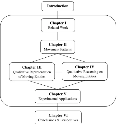
5 Thesis Structure
The remainder of this thesis is organized as follows:
Chapter I discusses the relevant literature background for the subsequent approaches. Current formalisms and spatial models oriented to the representation of spatial and temporal relations, theoretical supports and formal modelling and reasoning approaches developed for a representation of qualitative movement, as well as current spatial models for the representation of topological relations under uncertainty are studied.
Chapter II introduces a series of topological properties that describe the spatial configuration of a directed line with respect to a region in a two-dimensional space. The movement patterns of moving entities are modelled based on boundary of the reference region and the orientation relations, respectively.
Chapter III introduces two formal models for a qualitative movement representation of a moving entity which is characterized either as spatially extended or as a point.
Chapter IV develops some reasoning mechanisms for the manipulation of entity movements in case of incomplete knowledge. We apply the notion of conceptual neighborhood diagram and composition tables. A series of case studies illustrate the whole approach.
Chapter V presents an application of the modelling approach to the aviation and maritime domains. The trajectories of either a plane or a vessel are modelled, analyzed, this offering several reasoning opportunities based on our approach.
Chapter VI. While each chapter contains a summary of its results, this concluding chapter lists the contributions of the thesis as a whole and provides a series of possible extension and application of our research.
Figure 2 General outline of the thesis Chapter IV Qualitative Reasoning on Moving Entities Chapter V Experimental Applications Chapter VI
Conclusions & Perspectives
Introduction Chapter I Related Work Chapter II Movement Patterns Chapter III Qualitative Representation of Moving Entities
Related Work
I.1 INTRODUCTION ... 10
I.2 QUALITATIVE SPATIAL AND TEMPORAL REPRESENTATIONS ... 10
2.1 QUALITATIVE TOPOLOGICAL RELATIONS ... 11 2.2 QUALITATIVE ORIENTATION RELATIONS ... 15 2.3 QUALITATIVE DISTANCE RELATIONS... 18 2.4 QUALITATIVE TEMPORAL RELATIONS ... 20
I.3 QUALITATIVE SPATIO-TEMPORAL REASONING ... 21
3.1 CONCEPTUAL NEIGHBOURHOODS ... 22 3.2 COMPOSITION TABLES ... 23
I.4 QUALITATIVE MOVEMENT MODELLING ... 25
4.1 SPACE +TIME APPROACHES ... 26 4.2 INTEGRATED SPACE-TIME APPROACHES ... 28
I.5 MOVEMENT SEMANTICS ... 30 I.6 DISCUSSION ... 32
Chapter
I.1 Introduction
This chapter presents a brief review of a series of research contributions closely related to our research. The chapter successively introduces recent work on the development of qualitative spatial and temporal representations, spatio-temporal reasoning mechanisms, qualitative representations of movement and semantic-based movement approaches. This chapter is by no means an exhaustive overview but merely points out some of the most noteworthy approaches that have influenced our work. The whole contributions are summarized in the conclusion of the chapter.
I.2 Qualitative Spatial and Temporal Representations
Qualitative calculi usually deal with elementary spatial entities (e.g., points, regions) and
qualitative relations between them (e.g., “touch”, “to the right of”). This is one the reasons
why qualitative representations are generally well understood by humans. However, it appears that the modelling of spatial qualitative relations, when combined with the temporal dimension, is not a straightforward task (Peuquet and Duan 1995). This stresses
a need for the development of knowledge representations that should support humans’
knowledge representations of spatial, temporal and spatio-temporal information. By imposing discrete and symbolic frameworks on real-world phenomena, qualitative spatio-temporal representations are likely to provide a bridge between the perceptual and conceptual levels, and then a formal and computational support for qualitative spatio-temporal reasoning.
Within GIS, real-world phenomena are usually represented by two sorts of conceptual realms: continuous and discrete. While continuous approaches generally provide structural representations based on either regular or irregular tessellations and the distribution of a continuous variable that can be mathematically modelled or approximated in some specific cases, discrete approaches represent spatial entities by appropriate geometrical primitives (e.g., points, lines, polygons) and some structural properties and relations (e.g.,
topological and orientation relations) (Latecki 1998).In fact, and due to a certain degree of
variability and uncertainty in the perception and abstraction of many real-world phenomena, the spatial entities that emerge according to a given domain of study can be considered as either well-defined (i.e., crisps) or fuzzy entities (Leung and Yan, 1997). In
the context of our research, the focus is on well-defined and precisely defined spatial entities.
2.1 Qualitative Topological Relations
One of the most foundational qualitative representations of space has been based on topology. Topology, also known as rubber sheet geometry (Vieu 1997), is mainly concerned with the properties of geometric objects (such as dimensionality, boundaries, and number of holes) that are invariant under some homeomorphisms such as translation, rotation and scaling. Several properties, so-called invariants, are preserved by topological transformations such as dimension, connectivity, separation and intersection. For instance, if there is a drawing on a rubber sheet, the topological properties of the drawing remain unchanged when the rubber sheet is distorted by stretching, twisting, or bending. However, other transformations such as tearing, puncturing, or inducing self-intersection do affect topological properties and relations (Mortensen 1997).
Over the last three decades, a large variety of formal approaches oriented to the representation of topological relations have been proposed by many scholars from a variety of fields and extensively applied to the representation of topological information within spatio-temporal databases (Güting and Schneider 2005; Tossebro 2011), spatial reasoning in artificial intelligence (Li and Cohn 2012), and representation of natural-language relations (Xu 2007; Praing and Schneider 2009) to mention a few examples. Most of these approaches can be classified into two categories, i.e., region-based and point set approaches. In the former approaches a spatial entity is considered as a whole, while in the latter approaches a spatial entity is represented in terms of the set of its components. According to the dimension of the spatial entities considered in a two-dimensional vector
space (IR2), six types of spatial configuration can be distinguished, including point-point,
point-line, point-region, line-line, line-region and region-region. As the configurations involving point objects (i.e. point-point, point-line and point-region) are relatively straightforward, most of the efforts have been oriented to the cases involving lines or regions.
2.1.1 Region-based Approaches
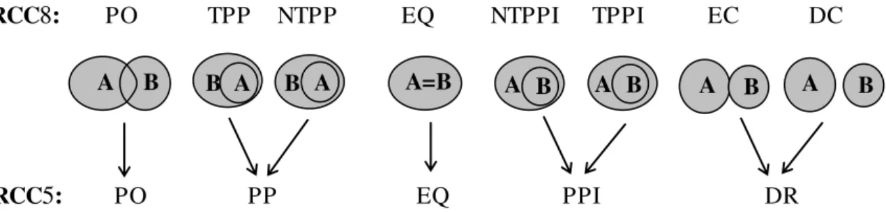
The region-based approaches take spatial regions as the basic modelling primitives. A spatial region is an atomic and non-null unit that cannot be subdivided into an interior and a boundary as permitted by point set topology. The best known approach is the Region
Connection Calculus (RCC) (Randell et al. 1992) which is developed on the spatial counterpart of the Interval Calculus applied to spatio-temporal reasoning (Clarke 1981; Clarke 1985) and based on the connection of entities. Connectivity is a fundamental relation in this context when determining whether and how two entities might interact.
The primitive relation in RCC is C(x,y), defined as region x connects with region y, which
holds when the regions x and y share a common point. Based on the primitive relation
C(x,y), a set of basic topological relations are defined (Table I.1) and has led to a rich
calculus of spatial predicates and relations.
Relation Interpretation Definition of R(x,y)
DC(x,y) x is disconnected from y C(x,y) P(x,y) x is a part of y z[C(z,x)C(z,y)] PP(x,y) x is a proper part of y P(x,y)P(y,x) EQ(x,y) x is identical with y P(x,y)P(y,x) O(x,y) x overlaps y z[P(z,x)P(z,y)] DR(x,y) x is discrete from y O(x,y) PO(x,y) x partially overlaps y O(x,y)P(x,y)P(y,x) EC(x,y) x is externally connected to y C(x,y)O(x,y)
TPP(x,y) x is a tangential proper part of y PP(x,y)z[EC(z,x)EC(z,y)]
NTPP(x,y) x is a nontangential proper part of y PP(x,y)z[EC(z,x)EC(z,y)]
Table I. 1 Topological relations defined from the connection C relation (Cohn et al. 1997)
The RCC calculus provides a powerful algebra to represent and make a difference
between complex entities such as doughnuts or loops (Gotts et al. 1996), as well as it has
been extended to the integration of uncertainty (Schockaert et al. 2009). By removing
redundant relations and using the converse relation of TPP and NTPP, the RCC8 calculus
is composed of eight mutually exclusive and jointly exhaustive relationships: DC, EC, PO,
EQ, TPP, NTPP, TPPI, NTPPI. If the boundary of the region is not considered, some of
the RCC8 relations are grouped and overall reduced to five relations, which is known as
Figure I.1 Graphic representation of the RCC calculus
2.1.2 Point-Set Approaches
Point-set approaches consider a set of points as the basic modelling primitive and define topological relations from point-set topology (Alexandroff 1961). A series of formal models of topological relations have been suggested, and where the main properties of the regions are the interior, boundary, exterior and the dimension of a set of points.
The 4-Intersection Model (4IM) (Egenhofer and Franzosa 1991) formally models topological relations between two spatial entities through the intersection sets of interiors and boundaries of two point sets. Considering empty and non-empty as the values of the intersections, the 4IM model can distinguish 2 cases of topological relations for the point-point group, 3 cases for the point-point-line group, 3 cases for the point-point-region group, 16 cases for the line-line group, 13 cases for the line-region group, and 8 cases for two simple regions (i.e., 2-dimensional connected regions with connected boundaries).
Egenhofer and Herring (1991) extended the 4IM to a 9-Intersection Model (9IM) taking into consideration exterior intersections. The 9IM can be regarded as a refinement of 4IM. Moreover, this binary topological relation model is also based on the concepts of point-set topology with open and closed sets. The binary topological relations between two spatial
entities, A and B, in IR2 are based upon the intersection of A’s interior (Ao), boundary (A),
and exterior (A–) with B’s interior (Bo), boundary (B), and exterior (B–). The nine
intersections between the respective entity’s parts are used for describing a topological
relation and can be concisely represented by a 3×3 matrix, i.e.,
B A B A B A B A B A B A B A B A B A B A M o o o o o o I( , ) 9 (I.1)
The 9IM can distinguish 29=512 types of binary topological relations. However, only a
small subset of them is plausible for spatial entities embedded in IR2 (Egenhofer and
Herring 1991; Clementini et al. 1993). For example, the 9IM can identify 2 cases for the
A B B A B A A=B A B A B a A B A B
RCC8: PO TPP NTPP EQ NTPPI TPPI EC DC
point-point group, 3 cases for the point-line group, 3 cases for the point-region group, 33 cases for line-line group, 19 cases for the line-region group, and 8 cases for region-region
group. The 8 topological relations between regions are: disjoint, overlaps, meets, equals,
inside, contains, covers, and covered-by. These correspond once more to the RCC
relations (Cohn 1996), with: disjoint = DC, overlaps = PO, meets = EC, equals = EQ,
inside = NTPP, contains = NTPPI, covers = TPP, and covered-by = TPPI.
Due to the fact that either 4IM or 9IM cannot identify the resulting dimension of the
intersections, Clementini et al. (1993) developed the Dimension Extended Model (DEM)
by deriving the dimension of the intersection set. This model may be represented by: ) ( ) ( ) ( ) ( ) , ( B A Dim B A Dim B A Dim B A Dim B A M o o o o D (I.2)
In Equation I.2, the dimension of intersections is defined by the following function, i.e.
Theoretically, there are 44=256 different topological cases that can be distinguished by
the DEM. However, geometric constraints for specific groups of relations can be applied to reduce the number of cases due to the fact that the dimension of the intersection cannot be higher than the lowest dimension of the two operands of the intersection. Taking the line-line group as an example, the dimension of the intersection of the interiors of two entities only possibly assumes the values: -1 and 0 due to the limit of the dimension of the entity itself. Regarding the DEM, 2 cases for the point group, 3 cases for the point-line group, 3 cases for the point-region group, 18 cases for the point-line-point-line group, 17 cases for the line-region group, and 9 cases for the region-region group can be identified. In order to provide a more user-oriented modelling method, the Calculus Based Method (CBM)
(Clementini et al. 1993) identified five topological relations under the condition that only
boundary operators are available: touch, in, cross, overlap, and disjoint. Clementini and Di
Felice (1994) proved that the CBM is more expressive than the 9IM or DEM and could be regarded as the minimal set to represent all 9IM and DEM relations.
Apart from these generic models that are nowadays considered as the main spatial reasoning references within GIS, other efforts have been made on the development of models dedicated to specific types of features, e.g. line-line relations (Clementini and Di
If the intersection set is empty
If the intersection set contains at least a point and no lines or areas If the intersection set contains at least a line and no areas
If the intersection set contains at least an area , 2 , 1 , 0 , 1 ) ( Dim
Felice 1998; Li and Deng 2006) and line-region relation models (Egenhofer and Franzosa 1995; Kurata and Egenhofer 2007; Deng 2008).
2.2 Qualitative Orientation Relations
Qualitative orientation relations describe how two spatial entities are placed one relative to the other. They can be defined in terms of three basic concepts: the primary object,
reference object and frame of reference (Clementini et al. 1997). Orientation relations are
important complementary qualitative relations because topological relations alone are insufficient in many situations as they cannot encompass all the semantics of a given spatial configuration.
Orientation relations can be defined as absolute orientations (e.g., cardinal) or relative orientations. By applying directional abstractions (e.g., North, Northeast, East, Southeast, South, Southwest, West, and Northwest), Frank (1991, 1992) divides the 2D space around a reference object into cone-shaped areas (Figure I.2a) or 4 partitions using a projection-based approach (Figure I.2b). Moreover a neutral zone, which is an area around the reference object where no direction is defined, can be added to divide the neighboring space into 9 areas (Figure I.2c). Then Frank (1996) compared the three representations and showed that the projection-based representation with a neutral zone was more efficient than the others in terms of spatial reasoning capabilities. Similar to the projection-based approach with a neutral zone, the direction-relation matrix (Goyal and Egenhofer, 2001) approximates the reference object by its minimum bounding rectangle and defines 9 regions around it. A 3×3 matrix (Equation I.3) is used to calculate the intersection of the primary region with the 9 regions.
) ( ) ( ) ( ) ( ) ( ) ( ) ( ) ( ) ( ) ( ) ( ) ( ( ) ) ( ) ( ) ( ) ( ) ( ) , ( B Area B SE Area B Area B S Area B Area B SW Area B Area B E Area B Area B O Area B Area B W Area B Area B NE Area B Area B N Area B Area B NW Area B A Dir A A A A A A A A A (I.3)
Figure I.2 Cardinal directions between two points in 2D space: (a) cone-based model; (b) projection-based model; (c) projection-based model with neutral zone
The calculi describing relative orientations are mainly based on three different kinds of primitive entities that are closely related: a tuple of points, directed line segment and oriented point. A tuple of points can be regarded as a line segment, a directed line segment
L can be represented by its start point sL and end point eL, while an oriented point can be
modelled as a directed line segment of infinitesimally small length.
An example of calculi based on point tuples is the Flip-Flop calculus (Ligozat 1993) which has been late refined to the LR calculus by Scivos and Nebel (2004). Further examples of calculi of this kind are single- and double-cross calculus (Freksa 1992b). The
Ternary Point Configuration Calculus (TPCC) (Moratz et al. 2003; Dylla and Moratz 2004)
is calculus based on ternary relations complemented by qualitative distance measurements based on two of the three points. A reference frame for the LR calculus is given by a tuple
of points A, B . For A≠ B, the frame is a directed line segment from A to B written as AB
as shown in Figure I.3. A ray being collinear to AB and having the same direction divides
the Euclidean plane into three sections: the half-plane to the left of the ray (l); the
half-plane to the right of the ray (r); and the ray itself. The ray itself is divided into segments
by points A and B: The segment behind A (b); the start point A (s); the segment in-between
A and B (i); the end point B (e) and the segment in front of B (f). Given a third point C, the
orientation relation R use the symbols introduced above can be written as
(ABRC) (I.4)
For example, in Figure I.3, C lies to the right of the ray, expressed as (ABrC). The seven
relations are defined by Flip-Flop calculus, in which the case of A = B are lacking. In that
case, dou for A = B≠ C and tri for A = B = C has been introduced in the LR calculus.
N NE NW W E SW S SE Neutral zone (c) (b) (a) N NE NW W E SW S SE N NW W E SW S SE NE
Figure I.3 LR relations
The arrangement of the intervals can be horizontal or vertical, and it is possible to change their orientations within a range of 360° in the two-dimensional plane. Gottfried (2004) provides a set of relations based on line segments to represent both positional and orientation information. Schlieder (1995) developed the Line Segment Calculus but
without the possibility to express polylines. Further refinements by Moratz et al. (2000)
lead to the Dipole Relation Algebra (DRA) with the ability to express relations and qualitative angles between line segments in any position. The reference frame of these calculi is a directed line segment (also called a dipole) in the Euclidean plane with
non-zero length. A dipole A is formed by a tuple of its start point and end point <sA, eA>. The
set of 7 different dipole-point relations are used to distinguish the location and orientation
of different dipoles. Take the DRAf (f stands for fine grained) in Figure I.4 as an example,
the relations between two dipoles may be specified according to the following four
relationships: A A B B AR e BR s BR e s R A 1 2 3 4 (I.5)
where Ri {l, r, b, s, i, e, f} with 1 i4. Theoretically this leads to 2401 relations, out of
which 72 relations are geometrically possible. DRAfp is an extension of DRAf with
additional qualitative angle information due to “parallelism”.
Figure I.4 DRA relations
The calculus that considers oriented points is the Oriented Point Relation Algebra
(Moratz 2006) which is abbreviated as OPRA or OPRAm, where mN is a parameter that
determines the granularity of the reference frames. The oriented point is based on the perception of a spatial entity (e.g., a car) moving in space with a certain direction. The
i e s l b A B C f r sA eA eB sB A B
motivation for this abstraction is quite the same as for the dipole calculi introduced above but it disregards any possible lengths of the entities. The oriented point is defined as a
tuple p,, where p is a coordinate in IR2 and an angle to an arbitrary but fixed axis.
The plane around each oriented point is sectioned by m lines with one of them having the
same orientation as the oriented point itself. The angles between all lines are equal. The linear sectors (on the lines) and planar sectors (between two lines) are numbered from 0 to
4m-1 counterclockwise. The label 0 is assigned to the orientation of the oriented point.
Given an oriented point A, an OPRA2 reference frame is constructed as the line through
the point A being collinear to its direction and a line through A being perpendicular to the
previous one as shown in Figure I.5. The plane is segmented into 4 linear and 4 planar sectors which are assigned numbers from 0 to 7 counterclockwise. For another oriented
point B, the same reference frame is also constructed. If A disjoint B, the OPRA2 relation
B A j
i
2 is defined according to the sector in which the oriented point lies: i is the sector of
the reference frame of A in which B lies and j is the sector of the reference frame of B in
which A lies. The relation in Figure I.5 is A 2B
7
2 . If A meet B, then i is set to s, and j is the
sector of the reference frame of A which B points into.
Figure I.5 OPRA2 relations
2.3 Qualitative Distance Relations
The perception of the concept of distance, which is a fundamental concept in everyday life, is closely dependent upon both culture and experience (Lowe and Moryadas 1975). On the one hand quantitative approaches avoid these contextual issues by reducing all distance information to an absolute metric scale. On the other hand, qualitative distance relations can be modelled by relative distances or by a combination of absolute and relative distances. An absolute distance between two spatial entities can be directly computed
based on their positions, while a relative distance can be obtained by comparing the
distance to a third entity, i.e. closer than, equidistant, or further than.
For the former approaches, Hernandez et al. (1995) introduces a relative set of distance
distinctions at different levels of granularity. This model makes a difference between close,
medium, and far, or a another level of granularity between five distinctions very close,
close, commensurate, far, and very far as illustrated in Figure I.6. Distance-based reasoning frameworks can be further refined by additional spatial relations. For instance,
Hernandez’s work has been extended by Clementini et al. (1997) to include orientation
relations. This model is made up of an ordered sequence of distance relations and a set of
orientation relations. Each distance relation is defined under an acceptance area which
can be uniquely identified with consecutive spatial intervals (0,1,,n) surrounding a
reference entity. The relations between si are defined according to the distance-based
relations, which can be used to specify a monotonicity property (i are increasing) (Figure
I.7a), or the order of magnitude relationships (i+j~i for j < i) (Figure I.7b). So far
several calculi have been suggested based on a primitive which combines both distance and orientation information. Zimmermann and Freksa (1993) introduced a primitive which defines the relative position of a point with respect to a directed line segment. Liu (1998) explicitly defined the semantics of qualitative distance and qualitative orientation angles to suggest a representation of qualitative trigonometry. Moratz and Wallgrün (2012) extended a point-based orientation calculi with a local reference distance which is referred to as elevation and express relative distance relations by comparing these elevations.
Figure I.7 Distance-based relations between is
2.4 Qualitative Temporal Relations
Time can be regarded as a projection of events that occur and properties that hold. Any sort of event or happening can be described by a corresponding time (Allen and Hayes 1989). Approaches oriented to the representation of temporal knowledge are mainly either point-based or interval-based. A time instant is a single, atomic time point in the time
domain (Jensen et al. 2009). The qualitative relations between time instants are (Vilain
and Kautz 1989): “ < ” (precedes), “ = ” (equals), and “ > ” (follows). Let us consider for
example two flight events as an example: “The aircraft AF1821 took off at CDG airport at
9:45 and landed in Rome at 11:55” and “The aircraft EI527 took off at CDG airport at
16:00 and landed in London at 17:10”. These events are associated with the following
temporal intervals [9:45, 11:55] and [16:00, 17:10], respectively. Time instants t1 (9:45)
and t2 (16:00) denote the “beginning of the flight” for each flight, respectively. This
denotes a transition from a motionless state to the flight being in progress, that is, a motion state.
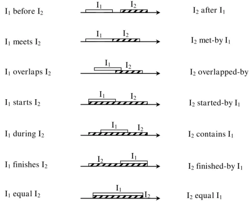
Many temporal representation frameworks such as the Situation Calculus (McCarthy and Hayes 1969) and the Time Specialist (Kahn and Gorry 1977) are based on time instants. On the other hand, taking intervals as a primitive for representing and reasoning has been also considered in temporal reasoning (Hamblin 1971; Humberstone 1979). The Interval Calculus (Allen 1983) provides a rich formalism to express qualitative relations between temporal intervals. Allen’s algebra has strongly influenced research in temporal, and even spatial and spatio-temporal reasoning.
Allen introduces a calculus based on binary relations between temporal intervals
without gaps plus a set of operations defined over these relations. A temporal interval I is
represented as a pair (I-, I+) of real numbers with I- < I+, which denote the beginning and
end points of the temporal interval, respectively. According to all possible relations
0 1 2 0 1 2 3 4 (a) (b)
between two temporal intervals based on the relative orderings of their beginning and end
points, 13 temporal relations which are so-called Allen’s basic relations are derived. As
shown in Figure I.8, these relations are composed of six temporal relations (before, meets,
overlaps, starts, during, finishes) and their inverse relations (after, met-by, overlapped-by,
started-by, contains, finished-by), and a self-inverse relation (equal).
Figure I.8 Thirteen temporal relations between two temporal intervals I1 and I2
I.3 Qualitative Spatio-Temporal Reasoning
One of the main objectives of Qualitative Spatio-Temporal Reasoning (QSTR) is to match
as much as possible humans’ common activities of their daily life, and more generally
real-world phenomena that deal with objects located in space and that change over time. Although formal models of spatial and temporal relations introduced in the previous sub-sections represent some basic spatial and temporal relations, the ability to reason on a given spatio-temporal system is a much more complicated task. The range of reasoning tasks related to humans’ activities or to the representation of real world phenomena is very large, this generating a need for the development of generic and domain-oriented algebra that can support modelling and reasoning tasks. Recent years have witnessed the developments of several QSTR frameworks oriented to the representation of
spatio-I1 I2 I1 I2 I1 I2 I1 I2 I1 I2 I1 I2 I2 I1 I1beforeI2 I2afterI1 I1meets I2 I2met-by I1 I1overlaps I2 I2overlapped-by I1 I1starts I2 I2started-by I1 I1during I2 I2contains I1 I2finished-by I1 I1finishes I2 I1equal I2 I2equal I1
temporal dynamics (Hazarika 2005; Bhatt 2010; Bhatt and Wallgrün 2014) or integration
of different levels of abstractions (Hornsby 2001; Mau et al. 2006). Those frameworks
cover and have been applied to a large range of applications such as robotics (Bedkowski
2013), risk events detection (Ligozat et al. 2009, 2011), archeology (Jeansoulin and Papini
2007), scene analysis (Bhatt and Dylla 2009), automatic surveillance (Dee et al. 2009) and
so on. Several practical software tools providing general consistency and constraint
satisfaction tasks have been developed, prime examples are the generic toolkit QAT for
n-ary calculi (Condotta et al. 2006), SparQ (Dylla et al. 2006), and GQR (Gantner et al.
2008).
Two main perspectives can be considered when reasoning with qualitative spatial data over time: one is to take a snapshot viewpoint and describe a dynamic behaviour as a set of temporal states, while another one represents a given phenomenon as spatio-temporal histories. Whatever the point of view (i.e., snapshot or histories), an important preliminary requirement of any QSTR is to first model things that happen with appropriate spatial and temporal information. Secondly, and by providing additional reasoning mechanisms, novel information can be derived from elementary configurations. In this section, the most frequently used approaches for qualitative reasoning, i.e. conceptual neighbourhoods and composition tables, are briefly introduced.
3.1 Conceptual Neighbourhoods
Under the assumption of continuous change, the term of conceptual neighbourhood is
defined as: “A set of relations between pairs of events forms a conceptual neighbourhood
if its elements are path-connected through conceptual neighbor relations” (Freksa 1992a).
A Conceptual neighborhood diagram (CND), whose alternative names are conceptual neighbourhood graphs, transition graphs, and continuity network, is a diagram in which spatial or temporal relations (or potentially any set of concepts in a certain domain) are “networked” according to their conceptual closeness, like the one shown in Figure I.9 for
the set of RCC8 relations between regions. Each node corresponds to a relation and each
link connects a pair of conceptual neighbors in a CND. If one relation holds at a particular time, then there are some continuous changes possible to lead to another relation in its neighborhood. All the intermediate relations must be passed through while changing from
any relation to another one in the CND. Taking the quantity space {−, 0, +} as an example,
Research on qualitative spatial and temporal reasoning often considers the construction and utilization of various kinds of CNDs. Most of the qualitative spatial and temporal calculi introduced in this chapter have also derived CNDs. To the best of our knowledge, the FROB program introduced in (Forbus 1982) was the first program to use a transition graph that combines spatial continuity constraints with dynamic constraints for reasoning about the movement of point objects in space. A well-known CND is the one applied by Freksa (1991) to interval relations as defined in (Allen 1983). Further examples of conceptual neighborhood diagrams applied to spatio-temporal relations have been applied
to cyclic temporal interval relations (Hornsby et al. 1999), topological relations between
regions (Egenhofer and Al-Taha 1992), lines and regions (Egenhofer and Mark 1995), and directed lines (Kurata and Egenhofer 2006).
The novel knowledge that can be derived from conceptual neighbourhoods of some given JEPD relations can be used to evaluate the possible changes of a relation or to measure the similarity among some relations (Schwering 2007). CNDs have also been
applied to build a qualitative spatial simulator (Cui et al. 1992) and to movement-based
reasoning (Egenhofer and Al-Taha 1992; Rajagopalan 1994; Van de Weghe 2004; Noyon
et al. 2007; Glez-Cabrera et al. 2013). Y X X Y Y X Y X X X X X Y Y Y Y Y DC EC PO TPP TPPI EQ NTPPI NTPP
Figure I.9 CND of RCC8 (Randell et al. 1992)
3.2 Composition Tables
Given a set of n jointly exhaustive and pairwise disjoint (JEPD) basic relations, the
algebraic operations union, intersection, complement, and converse of relations can be
computed. Taking the 13 basic temporal relations of Allen (1983) for example, these
operations are defined as follows (R1 and R2 being subsets of the 13 Allen relations):
The union (R1 + R2) of two sets R1 and R2 is the set-theoretic intersection of the two
Eg: If R1 = {before, meets}, R2 = {contains, finished-by},
then R1 + R2 = {before, meets, contains, finished-by }.
The intersection (R1 R2) of two sets R1 and R2 is the set-theoretic intersection of
the two relations; it is the relation composed of all basic relations that are in both
R1 and R2.
Eg: If R1 = {before, starts, during, finished-by}, R2 = {before, overlaps, contains},
then R1 R2 = {before}.
The complement (~R) of a set R is the relation consisting of all basic relations not
in R. For every relation R, ~ (~R) = R.
Eg: If R = {before, overlaps, during, started-by, contains},
then~R = {meets, starts, finishes, after, met-by, overlapped-by, finished-by}.
The converse (!R) of a set R is the relation consisting of the converses of all basic
relations in R. For every relation R, ! (!R) = R.
Eg: If R = {overlaps, contains},
then !R = {overlapped-by, during}.
The composition of binary relations, also called relative product (Tarski, 1941), is the
most prevalent operator used for QSTR to generate new relations, i.e., if two existing
relations R and S share a common entity, a composition can be derived and is denoted by:
} ) , ( ) , ( : | ) , {(x y z x z Rand z y S S R (I.6)
If there are no constraints imposed on the composition, this gives a universal disjunction U,
which is the disjunction of all relations of the JEPD set. By constructing a n n
composition table (also denoted as transitivity table), where the set of possible new relations are stored, the inference result can be preliminary evaluated instead of computing the possible resulting configurations. The composition tables have been precomputed for many different qualitative spatial and temporal calculus, e.g., temporal calculus (Allen
1983; Freksa 1992a), topological calculi (Cui et al. 1993; Egenhofer 1994), directional
calculi (Frank 1991; Freksa 1992b), distance calculi (Hernandez et al. 1995), and
spatio-temporal calculi (Van de Weghe 2004). Although the composition tables of the calculi based on ordered or well-structured domains are easy to construct, such as the Directed
Interval Algebra (Renz 2001) or the Rectangle Algebra (Balbiani et al. 1999), it is
generally difficult to compute the compositions effectively in many other cases especially for domains with arbitrary spatial regions such as those internally disconnected. In some domains, the operation of composition could lead to an infinite number of relations,
whereas the basic idea of qualitative reasoning is to deal with a finite number of relations (Renz and Ligozat 2005). Many researchers have pointed out that composition tables do not necessarily correspond to the formal definition of composition (Bennett 1994; Grigni
et al. 1995; Ligozat 2001). It can be resorted to a weaker form of composition in order to apply constraint-based reasoning mechanisms (Cohn and Renz 2008). The weak
composition table for RCC8 (Düntsch et al. 2001) is shown as Table I. 2. Further
composition tables can be found for topological relations (Hernandez 1994; Kurata and Egenhofer 2006), orientation relations (Frank 1992; Freksa 1992b; Hernandez 1994;
Papadias and Egenhofer 1997), distance relations (Hernandez et al. 1995) and temporal
relations (Allen 1983; Freksa 1992a).
DC EC PO TPP NTPP TPPI NTPPI EQ DC No info DR,PO, DR, PO, DR, PO, DR, PO, DC DC DC
PP PP PP PP
EC DR,PO, DR, PO, DR, PO, EC, PO, PO, PP DR DC EC PPI TPP,TPPI PP PP
PO DR,PO, DR, PO, No info PO,PP PO, PP DR, PO, DR, PO, PO PPI PPI PPI PPi
TPP DC DR DR, PO, PP NTPP DR, PO, DR, PO, TPP PP TPP ,TPI PPI
NTPP DC DC DR, PO, NTPP NTPP DR, PO, No info NTPP PPi PP
TPPI DR, PO, EC, PO, PO, PPI PO, TPP PO,PP PPI NTPPI TPPI PPI PPI TPPI
NTPPI DR, PO, PO, PPI PO, PPI PO, PPI PO NTPPI NTPPI NTPPI PPI
EQ DC EC PO TPP NTPP TPPI NTPPI EQ
Table I.2 Composition table for RCC8
I.4 Qualitative Movement Modelling
Instead of describing how objects are moving quantitatively, i.e. by lists of many precise positions, modelling movement in a qualitative way can formalize our common-sense view of the world. As topological, orientation, and distance relations between some spatial entities are likely to change over time, the formal models of spatial relations introduced above are not sufficient as such to represent the spatio-temporal behaviour of these spatial entities. The notion of movement closely associated to a given spatial entity is a
fundamental concept that can model and embed its behaviour in space and time. This can also denote the notion of spatial change associated to a given spatial entity. Such changes intuitively perceived by humans as qualitative processes and have been elsewhere studied by Naive Physics in an absolute space to formalize common sense human beings knowledge of physical world (Hayes 1979). Several formal approaches have been then developed such as the Qualitative Process Theory (Forbus 1982, 1983), Qualitative
Kinematics (Forbus et al. 1987; Faltings 1990), and Region-Based Geometry (Bennett et
al. 2000). Most of these qualitative models focus on how entities move one in relation to
the others. This section reviews current approaches oriented to qualitative and relative movement descriptions, those being translation-, rotation- and scale-invariant. A few key factors that differentiate those modelling approaches are as follows:
Whether they consider dimensionless points or regions as primitive objects, either in time, space or in space and time.
Whether they are based on discrete or continuous times.
Whether they represent the space and time domains separately or homogeneously. We classified those modelling approaches into two groups: one denotes approaches which represent two separated domains for space and time, and the other approaches which integrate a primitive and integrated space-time domain.
4.1 Space + Time Approaches
Let us first consider formal models that consider space and time as separate domains. Those approaches model movement as a sequence of locations. A movement is either modelled as a change associated to time instants (i.e., that denotes an instance or a state)
(Gottfried 2004; Noyon et al. 2007; Gottfried 2011; Glez-Cabrera et al., 2013) or to pairs
of adjacent time intervals (Van de Weghe 2004).
The Qualitative Trajectory Calculus (QTC) (Van de Weghe 2004) is in fact a set of calculi that represents the relative movement of some spatial objects. The QTC-Basic
(QTCB) considers a notion of a qualitative distance between a pair of moving points, such
as moving towards or moving away from (Van de Weghe et al. 2005, 2006). The more
general QTC-Double-Cross calculus (QTCC) takes into account the relative orientation of
the entity movements in a 2-dimensional space, and represents the relative movement of
two entities by a four-component label. The first two components describe a distance
change trend of an entity with respect to the current position of another entity, while the other two components describe the relative orientation of the entity movements with
respect to the reference line that connects them. The QTC on Networks (Delafontaine et al.
2008), i.e. QTCN and QTCDN, represent the qualitative relation between two moving
entities in a static and dynamic network, respectively. More precisely, one or more of the
following parameters are applied to describe the situation of two moving points A and B at
two successive time instants t and t+1.
the relative distance: one of the points approaches (−), moves away from (+), or keeps the same distance from the other (0);
the relative speed: the speed of Ais smaller (−), larger (+), or equal (0) to that of B;
the orientation relation: each point moves towards the left half-plane (−), towards the right half-plane (+), or moves while staying on the line (0).
Take Figure I.10 as an example, the relations between A and B can be denoted as A (−,
+, +, −, −) B according to the QTCC calculus (A approaches B, B moves away from A, A
moves toward the right half-plane, B toward the left half-plane, and the speed of A is less
than that of B).
Figure I.10 Illustration of QTC
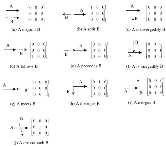
When considering the start point and the end point as the boundary of a directed line
segment, the 9IM (Egenhofer and Herring 1991) is extended to 9+IM (Kurata and
Egenhofer 2007), in which 26 topological relations are defined between a directed line and a region for characterizing movement patterns. In order to describe the properties of these
topological relations, they denote by I, B, E the entity’s positions in the region’s interior,
boundary, and exterior, respectively.
To qualify the movement of a former entity with reference to a latter one as perceived
by an observer acting in the environment, Noyon et al. (2007) proposed a formal
trajectory model based on two elementary primitives: relative velocity and relative
position. The trajectory configurations illustrated in Figure I.11 are an example of the
configuration A(v+p+)B when B is either a point (Figure I.11a), a line (Figure I.11b), or a
polygon (Figure I.11c) where the relative velocity is positive (the reference object A is
faster than the target object B), and B disjoint A. The formal identification of elementary